Note: Descriptions are shown in the official language in which they were submitted.
CA 02203776 1999-07-29
"CONCURRENT LEARNING AND PERFORMANCE
INFORMATION PROCESSING SYSTEM"
FIELD OF INVENTION
5 Generally, the present invention relates to the field of
parallel processing neurocomputing systems and more particularly to
real-time parallel processing in which learning and performance
occur during a sequence of measurement trials.
BACKGROUND
Conventional statistics software and conventional neural
network software identify input-output relationships during a training
phase and apply the learned input-output relationships during a
performance phase. For example, during the training phase a neural
1 5 network adjusts connection weights until known target output values
are produced from known input values. During the performance
phase, the neural network uses connection weights identified during
the training phase to impute unknown output values from known
input values.
2 0 A conventional neural network consists of simple
interconnected processing elements. The basic operation of each
processing element is the transformation of its input signals to a
useful output signal. Each interconnection transmits signals from one
element to another element, with a relative effect on the output signal
2 5 that depends on the weight for the particular interconnection. A
conventional neural network may be trained by providing known
input values and output values to the network, which causes the
interconnection weights to be changed.
A variety of conventional neural network learning
3 0 methods and models have been developed for massively parallel
processing. Among these methods and models, baekpropagation is the
most widely used learning method and the multi-layer perception is
the most widely used model. Mufti-layer perceptions have two or
more processing element layers, most commonly an input layer, a
3 5 single hidden layer and an output layer. The hidden layer contains
CA 02203776 1997-04-25
WO 96/14616 PCT/US95/14160
a
processing elements that enable conventional neural networks to
identify nonlinear input-output relationships.
Conventional neural network learning and performing
operations can be performed quickly during each respective stage,
because neural network processing elements can perform in parallel.
Conventional neural network accuracy depends on daoa predictability
and network structure that are prespecified by the user, including the
number of layers and the number of processing elements in each
layer.
1 0 Conventional neural network learning occurs when a set
of training records is imposed on the network, with each such record
containing fixed input and output values. The network uses each
record to update the network's learning by first computing network
outputs as a function of the record inputs along with connection
1 5 weights and other parameters that have been learned up to that point.
The weights are then adjusted depending on the closeness of the
computed output values to the training record output values. For
example, suppose that a trained output value is 1.0 and the network
computed value is 0.4. The network error will be 0.6 (1.0 - 0.4 =
2 0 0.6), which will be used to determine the weight adjustments
necessary for minilr~izing the error. Training occurs by adjusting
weights in the same way until all such training records have been
used, after which the process is repeated until all error values have
been sufficiently reduced.
2 5 Conventional neural network training and performance
phases differ in two basic ways. While weight values change during
training to decrease errors between training and computed outputs,
weight values are fixed during the performance phase. Additionally,
output values are known during the training phase, but output values
3 0 can only be predicted during the performance phase. The predicted
output values are a function of performance phase input values and
connection weight values that were learned during the training phase.
While input-output relationship identification through
conventional statistical analysis and neural network analysis may be
3 5 satisfactory for some applications, both such approaches have limited
utility in other applications. Effective manual data analysis requires
extensive training and experience, along with time-consuming effort.
Conventional neural network analysis requires less training and
CA 02203776 1999-07-29
3
effort, although the results produced by conventional neural networks
are less reliable and harder to interpret than manual results.
A deficiency of both conventional statistics methods and
conventional neural network methods results from the distinct
5 training and performance phases implemented by each method.
Requiring two distinct phases causes considerable learning time to be
spent before performance can begin. Training delays occur in
manual statistics methods because even trained expert analysis takes
considerable time, and training delays occur in neural network
1 0 methods because many training passes through numerous training
records are needed. Thus, conventional statistical analysis is limited
to settings where (a) delays are acceptable between the time learning
occurs and the time learned models are used, and (b) input-output
relationships are stable between the time training analysis begins and
1 5 performance operations begin.
Thus, there is a need in the art for an information
processing system that may operate quickly to either learn or perform
or both within any time trial.
2 0 SUMMARY OF THE INVENTION
Generally described, the present invention provides a
data analysis system that receives measured input values for variables
during a time trial and (learns) relationships among the variables
gradually by improving learned relationships from trial to trial.
2 S Additionally, if any input values are missing, the present invention
provides, during the time trial, an expected (imputed) output values
for the missing value that is based on the prior learned relationships
among the analyzed variables.
More particularly, the present invention provides the
3 0 imputed values, by implementing a mathematical regression analysis of
feature values that are predetermined functions of the input values.
The regression analysis is performed by utilizing a matrix of
connection weights to predict each feature value as a weighted sum of
other feature values. Connection weight elements are updated during
3 5 each trial to reflect new connection weight information from trial
input measurements. Also, a component learning weight is also
utilized during each trial that determines the amount of impact that
CA 02203776 1999-07-29
4
the input measurement vector has on learning relative to prior vectors
received. With respect to embodiments, the present invention may
process the input values in parallel or process the values sequentially.
The different input values may be provided in the form of vectors.
5 Each of the values of the input feature vector is operated on
individually with respect to prior learned parameters. In the parallel
embodiment, a plurality of processors process the input values, with
each processor dedicated to receive a specific input value from the
vector. That is, if the system is set up to receive sixteen input feature
1 0 values (i.e., corresponding to a vector of length sixteen), sixteen
processing units are used to process the input feature values
simultaneously. In the sequential embodiment, one processor is
provided to successively process each of the input feature values.
In the parallel embodiment of the present invention,
1 5 each of the processing units is operative to receive, during a time
trial, individual input values from an input vector. A plurality of
conductors connect each of the processing units to every other
processing unit of the system. The conductors transfer weighted
values among each of the processor unit according to processes of
2 0 the present invention. Each of the processing units provide, during
said time trial, an imputed output value based upon the weighted
values. Also, during the same time trial, each of the processing units
is operative to update connection weights for computing the weighted
values based on the input values received.
2 5 Due to the limited number of outputs that a particular
processor may drive, when interconnecting many processing units in
parallel for the processing of data, the number of processing units
that may be interconnected or driven by a single processing unit can
be substantially limited. However, the present invention provides a
3 0 plurality of switching junctions located along the conductor
interconnecting to alleviate the problem associated with a single
processor communicating with many others. The switching junctions
are operable for uniquely pairing each of the processors to every
other processor of the system. The present invention further
3 5 provides memory elements that are coupled to the switching
junctions. Each of the memory elements is individually coupled to
a separate switching junction and each of the memory elements
CA 02203776 1997-04-26 ~ ,~r;~D~' ~ ~ ~.1 ~ 16 0
s ~~~~5 =2 3 SEP 19'6
contains a connection weight value. Preferably, the connection
weight memory elements, located at the switching junctions, are the
connection weight elements of the matrix used in computing an
output value.
s The switching junctions may be operative to selectively
connect each of the processors to only one other processor at a time,
thereby forming multiple paired sets of the processors for
communicating the weight values during the time interval.
Preferably, the switching junctions successively connect different sets
w 1 0 of said multiple paired sets of the processors during multiple time
intervals. Also, the switching junctions are preferably operative to
connect the different sets of multiple paired processors in all possible
combinations in the minimum number of steps. A control unit is
operative to provide switching signals to the switching junctions in
1 s order to control the transfer of weighted values among the
processors. The conductors though which processor communication
occurs preferably are provided in a first conductor layer and a
second conductor layer, with the first and second conductor layers
operable for a connection at the switching junctions.
-.-- 2 0 The present invention may be implemented in a
sequential manner in which a conventional computer processing unit
may be used along with a conventional computer memory unit to
process input values. The sequential embodiment of the present
invention similarly computes output values from input values
2 s received during a time trial. In the sequential system, the processing
unit is operative to sequentially receive input values from an input
vector. Differing from the parallel embodiment, the elements of the
connections weight matrix are stored in sequential order as a data
string in a memory unit.
3 0 The processing unit of the sequential system is operative
to provide, during the time trial, an imputed output value based on
the elements of the connection weight matrix and is operative to
update the element of the connection weight matrix during the time
trial. Unlike conventional systems that would operate on connection
3 s weight as elements of a two-dimensional array, the sequential system
quickly operates on each element of the connection weight matrix in
AA~AInrn n. ,......_
CA 02203776 1999-07-29
6
a specially designed sequence. In conventional systems because
matrix multiplication operations are generally nested access loops
(one for the rows and one for the columns) concurrent operations
are slower than the sequential embodiment method of the present
$ invention.
The present invention also provides a system for
updating a connection weight matrix during each trial. Included in
the system for updating a connection weight matrix is a processing
unit operative to receive values from an input feature vector during
1 0 a time trial and a memory unit that contains connection weight
elements that identify a relationship among feature variables. The
processing unit is operative to update the connection weight elements
based on non-missing values of the input vector received. Unlike
other systems, the processing unit of the present invention is
1 S operative to update the connection weight elements based on a
component learning weight that is a distinct learning weight for each
input vector received. By using the component learning weight,
accurate relationships among feature variables may be determined.
Additionally, in both the parallel embodiment and the
2 0 sequential embodiment of the present invention, output values and
learned values may be evaluated and controlled by controller units
within the information processing system. A learning weight
controller may be provided that automatically adjusts the learning
weight from trial to trial in a manner that generally regulates the
2 5 relative effect that each input vector has on prior learning.
Additionally, a user may interface with the system to provide desired
learning weights different than the learning weights that may be
automatically provided by the system. Also, the present invention
may provide a feature function controller that is operative to convert
3 0 measurement values initially received by the system to input feature
vectors for imputing and learning use by the system. The feature
function controller is also operative to either provide default initial
connection weights or receive connection weight elements externally
so that a user of the system may supply initial weights as desired.
3 S Additionally, the learning weight controller may disable
the learning function of the computer system if an abnormal
CA 02203776 1999-07-29
7
deviation of input values occur. Also, the feature function controller
is operative to create a variety of statistics such as the first-order
difference between a current measurement value and the
corresponding measurement values stored from previous trials to
5 identify a sudden change in measurement values. A sudden change in
input values may indicate that an instrument from which the. input
values are received is faulty.
In addition to the physical embodiments of the present
invention, several processes are performed by the present invention.
1 0 The processes of the present invention include: receiving, at a
processing unit, an input vector m (IN)(f) during a time trial;
computing, during the time trial, an output value from a missing
input value of the input vector based on connection weight elements;
and updating, during the time trial, the connection weight elements
1 5 based on input values of the input vector.
The processes of the present invention may further
include the step of updating the connection weight elements based on
the component learning weight element discussed above. The
learning weight element may be calculated by: receiving a global
2 0 learning weight 1; receiving a learning history parameter ~, that is an
indicator of the prior learning weights of each input vector;
receiving a viability vector v(~, that indicates the extent to which an
input feature vector is missing; and multiplying those values together
to obtain the learning component weight (i.e., 1(C) (~ =1 v (~ 1(~).
2 5 The present invention is enabled to quickly update the
connection weight matrix during the same trial in which the system
imputes a value by utilizing as part of the connection weight updating
process a mean vector/t(OUT), of all feature vectors received. By
utilizing an input prior mean vector for the calculation of various
3 0 output values and parameters of the system, updating may occur
quickly. The prior mean vector ~ (IN), equals a (OUT) from the
previous measurement trial. If the process is in the first trial, then
~ (IN) may equal a system default value, preferably the value 1.0 for
a user-supplied value. The elements of ,u(OUT) calculated by the
3 5 following process equation:
a (OUT)( _ ( I(C)(~ m(IN)(f) + ~t (IN)(~ ) / ( 1 + 1(C)(~ ).
CA 02203776 1999-07-29
g
Processes of the present invention also include updating
the connection weight elements utilizing an intermediate imputed
vector, e(IN). Elements of the e(IN) vector may be calculated by the
following equation:
e(IN)(~ = v(~ ( m(IN)(~ - ~ (IN)(~ ) / ( 1 + 1(C)(~ ).
. The connection weight matrix may be updated utilizing
. ~ 1 0 the following process equations:
w (OUT) _ ( 1 + 1 ) ( m (IN) - c x T x ),
where
c=1( 1+l)l( 1+l( 1+1)d
1 5 x = e(IN) ~ (IN)
and
d = e(IN) m (IN) e(IN)T = x e(IN)T .
In the updating process, cv (IN) = r~ (OUT) from the previous trial.
If the current trial is the first trial, then w (IN) may equal a system
2 0 default value, preferably equals the identity matrix w or a user-
supplied value.
During the imputing process, the elements of the imputed
output vector ne (OUT) are calculated according to the following
process equation:
m(OUT)(~ _ ~ (IN)(~ + e(IN)(~( 2 - v(~ ) + x(~( v(~ - 1 ) /
.~, (fsfj
Other values utilized by the processes of the present invention are
described in further detail below.
3 0 Additionally, the present invention provides a method of
accessing multiple pairs of processors for computing the x vector.
The process includes accessing multiple sets of uniquely paired
processors during a time interval; retrieving each of the connection
weight elements, located at the switching junctions that connect the
3 5 paired processor units; and transferring e(IN)(~ located in each
processor to the other processor connected at the switching junction;
CA 02203776 1997-04-26
t~.~ .~3 SEP ]9~~
9 .
then computing a running sum of e(IN)m (IN) until all processor
pairs of the system have computed their corresponding values for x.
The processes of the present invention also provide a
method of accessing each set of processors for updating connection
weight elements. The process includes accessing multiple sets of
uniquely paired processors during a time interval; retrieving, by one
of the processors located at the switching junction, the connection
weight element located at the switching junction; updating the
connection weight element by the processor that retrieved the
1 0 connection weight element; and transferring the updated connection
weight element back to the memory element of the switching
junction.
Thus, it is an object of the present to provide an
information processing system that provides accurate learning based
1 5 on input values received.
It is a further object of the present invention to convert
input measurement values to input feature values during a single time
trial.
It is a further object of the present invention to provide
2 0 learning and performance (measurement and feature value imputing)
during a single time trial.
It is a further object of the present invention to impute
missing values from non-missing values.
It is a further object of the present invention to identify
2 5 unusual input feature deviations.
It is a further object of the present invention to provide
a system for learning and performing quickly during a single time
trial.
It is a further object of the present invention to identify
3 0 sudden changes in input feature values.
It is a further object of the present invention to provide
a system for quickly processing input feature values in parallel.
CA 02203776 1997-04-25
WO 96114616 PCT/US95/14160
/D
It is a further object of the present invention to provide
a system for quickly processing input feature values sequentially.
It is a further object of the present invention to provide
a system that enables multiple parallel processing units to
communicate among each of the processing units of the system
quickly.
It is a further object of the present invention to provide
a system that enables multiple parallel processing units to be accessed
in pairs.
1 0 It is a further object of the present invention to provide
communication between paired processors in a minimal number of
steps.
It is a further object of the present invention to provide
processes that accomplish the above objectives.
1 5 These and other objects, features, and advantages of the present
invention will become apparent from reading the following description in
conjunction with the accompanying drawings.
BRIEF DESCRIPTION OF THE DRAWINGS
2 0 Figure 1 illustrates the preferred embodiment of the
present invention.
Figure 2 is a block diagram that illustrates a parallel
processor embodiment of the preferred embodiment of the present
invention.
2 5 Figure 3 is a block diagram that illustrates a sequential
computer embodiment of the preferred embodiment of the present
invention.
Figure 4 shows an array of pixel values that may be
operated on by the preferred embodiment of the present invention.
3 0 Figure 5 shows a circuit layout for the joint access
memory and processors used in the parallel embodiment of the
present invention.
Figure 6a shows switching detail for a node in the joint
access memory of the preferred embodiment of the present invention.
CA 02203776 1997-04-25
WO 96/14616 PCT/US95/14160
Il
Figure 6b shows a side view of switching detail for a
node in the joint access memory of the preferred embodiment of the
present invention.
Figure 7 shows timing diagrams for joint access memory
control during intermediate matrix/vector operations of the parallel
embodiment .
Figure 8 shows timing diagrams for joint access memory
control timing for updating operations associated with a switching
junction of the joint access memory of the preferred embodiment of
1 0 the present invention.
Figure 9 shows processing time interval coordination for
parallel embodiment of the preferred embodiment of the present
invention.
Figure 10 shows a block diagram of the overall system
1 5 implerr :ed in the parallel embodiment of the preferred
embodiment of the present invention.
Figure 11 shows a block diagram of the overall system
implemented in the sequential embodiment of the preferred
embodiment of the present invention.
2 0 Figure 12 shows communication connections for
a
controller used in the parallel embodiment of the preferred
embodiment of the present invention.
Figure 13 shows communication connections for another
controller used in the parallel embodiment of the preferred
2 5 embodiment of the present invention.
Figures 14 through 22 are flow diagrams showing
preferred steps for the processes implemented by the preferred
embodiment of the present invention.
3 0 DETAILED DESCRIPTION
OPERATIONAL OVERVIEW
Referring to the figures, in which like numerals refer to
like pans throughout the several views, a concurrent learning and
performance information processing (CIP) neurocomputing system
3 5 made according to the preferred embodiment of the present invention
is shown. Referring to Figure 1, a CIP system 10 is implemented
CA 02203776 1997-04-25
WO 96/14616 PCT/US95/14160
with a coiiputer 12 connected to a display monitor 14. The computer
12 of the CIP system 10 receives data for evaluation from a data
acquisition device (DAD) 15, which may provide multiple
measurement values at time points via a connection line 16. Data
acquisition devices such as data acquisition computer boards and
related software are commercially available from companies such as
National Instruments Corporation. The computer 12 may also
receive input data and/or operation specifications from a conventional
keypad 17 via an input line 18. Receiving and responding to a set of
1 0 input measurement values at a time point is referred to herein as a
trial, and the set of input values is referred to herein as a
measurement record.
Generally, when the CIP system 10 receives an input
measurement record, the system determines (learns) the relationships
1 S that exist among the measurements received during the trials. If some
measurement valves are missing during the trial, the CIP system 10
provides imputed values that would be expected based on the prior
learned relationships among prior measurements along with the non-
missing current measurement values.
2 0 The CIP system 10 receives a measurement record from
the data acquisition device 15 and converts the measurement values to
feature values. The conversation of measurement values to feature
values operates to reduce the number of learned parameters that are
needed for learning or imputing. The feature values and other values
2 S calculated from the feature values provide useful data for predicting
or imputing values when certain measurement values are missing or
for determining that a monitored measurement value of a system has
abnormally deviated' from prior measurement values.
. Upon receiving an input measurement record at the
3 0 beginning of a trial, the CIP system 10 performs the following
operations as quickly as each input record arrives (i.e., system 10
performs concurrently): deriving input feature values from
incoming measurement values (concurrent data reduction);
identifying unusual input feature values or trends (concurrent
3 5 monitoring); estimating (i.e., imputing) missing feature values
(concurrent decision-making); and updating learned feature and
means, learned feature variances and learned interconnection weights
between features (concurrent teaming).
CA 02203776 1997-04-25
WO 96114616 PCT/US95/14160
!3
The CIP system is useful in many applications, such as
continuous and adaptive: (a) instrument monitoring in a chemically or
radioactively hostile environment; (b) on-board satellite measurement
monitoring; (c) missile tracking during unexpected excursions; (d) in-
s patient treatment monitoring; and (e) monitoring as well as
forecasting competitor pricing tactics. In some applications high
speed is less critical than in others. As a result, the CIP system has
provision for either embodiment on conventional (i.e., sequential)
computers or embodiment on faster parallel hardware.
1 0 Although speed is not a major concern in some
applications, CIP high speed is an advantage for broad utility.
Sequential CIP embodiment is faster than conventional statistics
counterparts for two reasons: first, the CIP system uses concurrent
updating instead of off-line training; second, the CIP system updates
1 5 the inverse of a certain covariance matrix directly, instead 'of the
conventional statistics practice of computing the covariance matrix
first and then inverting the covariance matrix. Concurrent matrix
inverse updating allows for fast CIP implementation. When
implemented using a sequential process, CIP response time increases
2 0 as the square of the number of data features utilized increases.
However, when implemented using a parallel process, CIP response
time increases only as the number of features utilized increases. In
the parallel system, a processor is provided for each feature. As a
result, parallel CIP response time is faster than sequential CIP
2 5 response time by a factor of the number of features utilized.
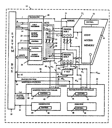
Parallel Svstem Overview
Referring to Figure 2, a parallel embodiments of the
basic subsystems of the CIP system 10 is shown. Before discussing
3 0 subsystem details, an operational CIP overview will be discussed with
reference to Figure 2. The CIP subsystems include a system bus 19, a
transducer 20, a kernel 21 and a manager 22. The transducer 20 and
the kernel 21 operate successively in order to accomplish the various
concurrent operations described above. Input measurement values
3 5 are first converted to input feature values by the transducer 20. The
input features are then processed by the kernel 21 to produce imputed
(i.e., output) features, updated learned parameters and monitoring
statistics. Output feature values are then converted to imputed (i.e.
CA 02203776 1997-04-26
S~~' l~~rv
1 4 ~~'~~ . . . _
output) measurement values by the transducer 20. The manager 22
coordinates transducer 20 and kernel 21 concurrent operations and
occasionally refines system operation.
The basic components of the transducer 20 are an input
processor 24 that has a recent feature memory (RFM) 25 and an
output processor 26. The input processor 24 and output processor
26
are each controlled by input and output control units 27 and 2$,
respectively. The recent feature memory 25 stores a preselected
number of input feature values m(IN), obtained from prior trials
(all
1 0 vectors in this document are row vectors). The stored recent
features
may be utilized in conjunction with input measurements j(IN) to
calculate, as discussed below, concurrent input feature values
m(IN)
for the current trial. At the beginning of each trial, the input
processor 24 receives an input measurement vector j(IN) and a
1 5 corresponding plausibility vector p. Plausibility vector elements
identify input measurement vector elements as non-missing or
missing.
The input processor 24 then (a) converts the input vector
j(IN) to some input features and combines those converted input
2 0 features with other converted features in the recent feature
memory
___ 25 to produce a resulting input feature vector m(IN); and (b)
converts
the plausibility vector p to a corresponding viability vector v.
Similar to the plausibility vector, the viability vector elements
identify
input feature vector elements as non-missing or missing. At the
end
2 5 of each trail, the output processor 26 receives an output feature
vector
m(OUT). The output processor 26 converts the output feature vector
m(OUT) to a corresponding output measurement vector j(OUT).
The input measurement vector j(IN) received by the
transducer input processor 24 contains the values of the input
3 0 measurement vectors from the DAD 15 (shown in Figure 1 ).
Plausibility values, provided either externally by the DAD 15 or
internally by the manager 22, indicate if a measurement plausibility
value is 0 (missing), 1 (non-missing) or some intermediate value
(a
combination of missing and non-missing quantum values as discussed
3 5 below). If an element of j(IN) is missing, as determined by the
corresponding element of p being 0, then the corresponding element
of j(OUT) is imputed, based on non-missing elements of j(IN) and/or
previously learned information. The imputing process utilizes
CA 02203776 1997-04-26
,, _ 9 m.~ m 6 0
1 $ '~'~~~3 SE~ 15~.ru
.,
measurement to feature conversion within the transducer input
processor 24, followed by missing feature value imputing within
the
kernel, followed by imputed feature to imputed measurement
conversion within the transducer output processor 26.
Prior to concurrent operation, the transducer input
processor 24 computes feature values and viability values
according to
functions that are determined by the manager 22. Each feature
element in m(IN) is a function of the measurement elements
in j(IN),
and each viability element of v is a corresponding function
of the
' ~' 1 0 plausibility elements in p. For example, the first feature
function in
m (IN) could be the sum, m (IN)( 1 ) = j(IN)( 1 ) + j(IN)(2),
and the
second feature function in m(IN) could be the product, m(IN)(2)
= j
(IN)(1) j IN)(3). Each feature viability value is the product
among
the plausibility values for the measurements that are independent
1 5 variables in the feature function. For example, if the
plausibility
values for the above three measurement functions are p(1)
= 1.0, p(2)
= 0.5 and p(3) = 0.0, then the two above feature viability
values will
bev(1)= 1.0x0.5=O.S,andv(2)=0.5x0.0=0Ø
Feature viability elements are computed as products of
2 0 corresponding measurement plausibility elements. Every CIP
system
input measurement value is treated as an average of non-missing
quantum measurement values from a larger set, some of which
may
be missing. The corresponding plausibility value of each input
measurement is further treated as the proportion of component
quanta
2 5 that are non-missing within the larger set. From probability
theory,
if an additive or product composite feature function is made
up of
several such input measurements and if the distributions of
missing
quanta are independent between measurements, the expected
proportion of terms in the composite for which all quantum
3 0 measurements are non-missing is the product of the component
measurement plausibility values. Since feature viability values
within
the CIP system have this expected proportion interpretation,
the
feature viability values are computed as products of component
measurement plausibility values.
3 5 After input measurement values j(IN) and plausibility
values p have been converted to input feature vectors m (IN)
and
viability values v by the transducer input processor 24, the
kernel 21
begins the next within-trial operation. Inputs to the kernel
21 include
CA 02203776 1997-04-26
pCTl~l~ 9 5 / .1 x.16 a
1 6 ~.~r~ ~~3 SEP 1~~
resulting feature values within m (IN), corresponding
viability values
within v and an input learning weight 1. The kernel 21
includes: a
processor 311 for feature 1 through processor 31p for
feature p; a
kernel control module 32; and a joint access memory (JAM)
23
connected by buses 45 through 45F, to the processors 31
through 31p.
Outputs from the kernel 21 include imputed feature values
in
m (OUT), feature function monitoring statistics that are
sent to the
and feature
manager via connections 411 , through 41 F and 41 JAM
,
value monitoring statistics that are sent to the manager
via connections
1 0 401 through 40p. The kernel processors 311 through 31p
use
preferably arithmetic logic units (ALUs) that implement
basic
arithmetic functions, in order to reduce the cost and
size of the
processors 311 through 31 F. As known to those skilled
in the art,
basic processors as such may be designed using commercially
1 5 available chip design software packages, such as Mentor
Graphics~, a
product of the Mentor Graphics Corporation.
Kernel processors 311 through 31F operate to: impute
missing feature values based on non-missing elements of
m (IN)
and/or previously learned kernel 21 parameters; update
learned
2 0 parameters that reside in each processor and in the joint
access
_. memory 23; and produce monitoring statistics for use by
the manager
22. As explained in more detail below, the kernel processors
311
through 31 p utilize two steps of inter-processor communication
to
transfer relevant values from each processor to every
other
2 S processor. Kernel processor operations also compute a
distance
measure d in the kernel distance ALU 34. Communication
between
the distance ALU 34 and each kernel processor occur through
connections 351 through 35p.
The kernel input learning weight l is a non-negative
3 0 number that - like input plausibility values and viability values - is
a quantum/probabilistic measure. The learning weight l for each trial
is treated by the CIP system as a ratio of quantum counts, the
numerator of which is the number of quantum measurement vectors
for the concurrent trial, and the denominator of which is the total of
3 5 all quantum measurements that have been used in prior learning.
Thus, if the concurrent input feature vector m(IN) has a high
learning weight l value, the input feature vector will have a larger
impact on learned parameter updating than if the input feature vector
CA 02203776 1997-04-26
~1'(t~95 I..~ 4.1~Q
~~~~~~23 SEP 1~;~
has a lower learning weight l value, because the input feature vector
m (IN) will contain a higher proportion of the resulting plausible
quantum measurement total. Normally, the learning weight l is
supplied as an input variable during each trial, but the learning weight
can also be generated optionally by the CIP system manager 32 as
discussed below.
Kernel imputing, memory updating and monitoring
operations are based on a statistical regression framework for
predicting missing features as additive functions of non-missing
1 0 feature values. Within the regression framework, the weights for
imputing each missing feature value from all others are well-known.
Formulation for the weights used for imputing are functions of
sample covariance matrix inverses. In the conventional approach to
regression, the F by F covariance matrix is computed first v based on
1 5 a training sample, followed by inverting the covariance matrix and
then computing regression weights as functions of the inverse. The
conventional approach involves storing and operating with a training
set that includes all measurements received up to the current input
trial. Storing all prior measurements is typical for conventional
2 0 systems, because all prior measurements are needed in order to first
calculate present covariances from which the inverse matrix may be
obtained.
Unlike conventional statistics operations, CIP kernel 21
operation does updates the inverse of v directly, based only on: (a)
2 5 the inverse of v and other parameters that have been learned up to
that trial; (b) incoming feature values m (IN); and (c) the input
learning weight 1. Consequently, CIP operations can keep up with
rapidly arriving information, without the need for either storing and
operating with a training data set or inverting a covariance matrix.
3 0 The process of updating the inverse elements of v is the
CIP counterpart to conventional learning. CIP fast updating
capability from trial to trial provides a statistically sound and fast
improvement to conventional learning from off-line training data. As
a result, the CIP System 10 provides an enhancement over the prior
3 5 art.
With continuous reference to Figure 2, the joint access
memory 23 contains the feature interconnection weights, one for each
of the possible F x (F -1)/2 pairs of features. The feature connection
CA 02203776 1997-04-26
~_'.. i ;~,;~~ 9 ~ j '~ r: ~ 6 ~'
1 s ~~~ ~2 S S~ P
weights correspond to the lower triangular elements of
v inverse.
The main diagonal elements of v inverse are also used
during kernel
imputing and feature function monitoring, and are modified
during
concurrent learning. Individual elements of the v inverse
main
diagonal reside in their corresponding kernel processor.
Once the kernel 21 has imputed feature values i n
m (OUT), the kernel sends the imputed feature vector m(OUT)
back
to the transducer output processor 24 via line 33, where
the imputed
feature values in m (OUT) are converted to imputed measurement
1 0 values in j(OUT) for system output by the transducer output
processor 26. In some modeling situations, only simple
output
conversions are needed. For example, if the CIP system
features
alternatively include the original measurements along
with product
functions of the original measurements, the output processor
26
1 5 converts imputed features to imputed measurements by excluding
all
but the imputed measurement set from the imputed feature
set. In
other modeling situations, more elaborate conversion may
be utilized.
For example, one CIP system feature alternative may convert
a set of
measurements to the average of the set of measurements
during
2 0 transducer input processing, in which case the transducer
output
_._ processor 26 sets all imputed output measurement values
to their
common imputed average value.
Once imputed measurement values j(OUT) have been
produced as outputs, the outputs can be useful in several
ways,
2 5 including: (a) replacing direct measurement values, such
as during
periods when instruments break down; (b) predicting measurement
values before the measurements occur, such as during econometric
forecasting operations; and (c) predicting measurement
values that
may never occur, such as during potentially faulty product
3 0 classification operations.
The manager 22 monitors and controls CIP system
operation. The subsystems of the manager 22 include: the
coordinator 38, which provides the CIP system-user interface;
the
executive 39, which dictates overall system control; the
learning
3 5 weight controller 40, which provides l to the kernel 21
in place of
externally supplied l values from the data acquisition
device 15
(Figure 1 ); and the feature function controller 41, which
establishes
and modifies measurement-feature function structure. In
CIP system
CA 02203776 1997-04-25
WO 96114616 PCT/US95/14160
concurrent operation, the kernel and transducer 20 modules are active
in a concurrent mode. When the system is operating in the
concurrent mode, the kernel 21 and transducer 20 operate
continuously based on input measurement values, plausibility values
and learning weights, according to system control parameters that are
set by the executive 48. These parameters include input
measurements specification, feature computing specifications, inter-
module buffering specifications and output measurement
specifications. During concurrent operation, the CIP system produces
1 0 imputed feature values, feature value monitoring statistics, updated
learned kernel parameter values and imputed output measurement
values.
The CIP system may also perform feature value
monitoring operations, which are performed by the kernel 21, the
1 5 learning weight controller 40 and the coordinator 49. During
feature value monitoring operations, each kernel processor 311
through 31F sends monitoring statistics via connections 401 through
40F to the manager 22. Deviance monitoring statistics are used
during each trial by the learning weight controller 40 within the
2 0 manager 22 to assess the extent that each feature is unexpected,
relative to: (a) the, mean value that has been computed from prior
learning for that feature, and (b) the value of that feature that would
be imputed if the feature was missing. Feature value statistics that are
sent from each kernel processor include the observed value, a Teamed
2 5 mean, a regressed value and a learned variance value for the feature .
of the processor. The learning weight controller 40 uses the feature
value monitoring statistics to compute concurrent feature deviance
measures. These deviance measures are then sent from the learning
weight controller 40 to the coordinator 38 to produce monitoring
3 0 graphics, which are then sent through the system bus 19 to the
monitor 14.
In addition to specifying feature imputing, feature value
monitoring and learned parameter updating operations concurrently,
the CIP manager 22 specifies feature function assessment and
3 5 assignment occasionally, and the CIP manager 22 controls learning
weight assignment alternatively. Feature function assessment and
assignment are performed by the feature function controller 41
within the manager 22, by simultaneously accessing the
CA 02203776 1997-04-25
WO 96/14616 PCTIUS95/14160
a°
interconnection weights in the joint access memory 23 through a
parallel port 41 JAM, along with other weights in processor 1 to
processor F through connections 411 to 41F. The feature function
controller 41 first examines the interconnection weights to identify
S features that are either redundant or unnecessary, that is, features that
do not provide information useful for learning and imputing. Feature
function controller 41 then commands the transducer input processor
24 to combine redundant features, remove unnecessary features or
add new features accordingly, through control lines 43.
1 0 As with CIP imputing and learned parameter updating
operations, CIP feature function monitoring and control operations
are based on a statistical regression framework. For example, all of
the necessary partial correlation coefficients and multiple correlation
coefficients for identifying redundant or unnecessary features can be
1 5 computed from the elements of v inverse that reside in the joint
access memory 23, and architectures closely resembling the kernel 21
architecture can be used to perform such refinement operations.
Although the refining operations are not performed as fast as
concurrent kernel 21 operations, the refining operations can be
2 0 performed almost as quickly and in concert with ongoing kernel 21
operations by using, parallel refinement processors as discussed below.
The probability/quantum basis for learning weight
interpretation allows learning weight schedules to be computed that
will produce: (a) equal impact learning, through which each input
2 5 feature vector will have the same overall impact on parameter
learning; (b) conservative learning, through which less recent input
feature vectors will have higher overall impact on parameter learning
than more recent input feature vectors; and (c) liberal learning,
through which more recent input feature vectors will have lower
3 0 overall impact. When the learning weight controller 40 is used to
supply learning weights to the CIP system in a basic form, the system
is programmed to only supply equal impact learning weights. In
another form, the learning weight controller 40 may use the CIP
system monitoring statistics to identify unusual trends in imputing
3 5 accuracy. If imputing accuracy drops sharply, the learning weight
controller 40 changes the learning weight computing schedule to
produce more liberal learning, based on the assumption that imputing
accuracy degradation is caused by a new set of circumstances that
CA 02203776 1997-04-26
r~.",23 SEP 1996
21
require previously learned parameters to be given less impact. The
learning weight may also modify elements of the plausibility vector p
if feature value monitoring indicates erratic measurement behavior.
Conventional Sec,~uential Computer System Overview
Referring to Figure 3, a block diagram illustrating the
CIP system 10 embodiment on a conventional computer with one
central processing unit is shown. The basic components of the
conventional sequential computer embodiment 12a of the sequential
1 0 CIP system 11 include: a transducer input 24a process; a kernel
process 21a; a transducer output process 26a; a coordinator 49a; an
executive 39a; a learning weight controller 40a; and a feature function
controller 41 a. Each of the components of the sequential CIP system
11 perform the same basic functions as the parallel CIP system 10.
1 5 However, in a conventional computer system, only one central
processor is utilized. Thus, in utilizing only one processor for kernel
31a operation, the time for processing input data takes more time to
implement than in the parallel CIP computing system 12.
Just as in the parallel system embodiment, the sequential
2 0 system receives an input vector j(IN) and a plausibility value p. As in
the parallel system, the input vectors ~'IN) are also converted to input
feature values m(IN). Plausibility values p are converted to viability
values v as discussed above. The kernel process 31a receives the
feature input value m(IN), the viability value, and a learning weight l
2 5 from the system. 'The kernel 21 a process produces an output feature
vector m(OUT) based upon connection weights stored in conventional
memory 301 that is allocated by the executive 39a. The output
feature vector m (OUT) is transferred to the output transducer 26a for
conversion to an output measurement value j(OUT) for external use,
3 0 as discussed above in connection with the CIP system 10.
The executive block 39a represents the sequential
computer main function and other blocks represent CIP subroutines.
Memory 301 for the kernel subroutine embodiment has conventional
data array form as known to those skilled in the art, and all shared
3 5 memory storage is allocated and maintained by the main executive
function. The executive 39a first initializes the CIP system by calling
the coordinator 39a subroutine, which in turn obtains user-supplied
system specifications, such as the length of the measurement vector
CA 02203776 1997-04-26 -
P~'I'9 5 l .~. x.16 ~~
2 2 ~..~3 CEP 1~~6
j(IN) and the number of feature functions, through the keyboard 18.
The executive 39a then allocates learned parameter memory and other
storage accordingly.
During each concurrent trial, the executive 39a program
calls the transducer input processor 24a subroutine, followed by the
kernel 21 a subroutine, which is followed by calling the transducer
output 26a subroutine. If the executive program 39a has been initially
set to do so, the executive 39a may also call the learning weight
controller 40a subroutine at the beginning of each trial to receive an
1 0 input learning weight l, and the executive may provide feature
monitoring statistics at the end of each trial to the coordinator 38a for
graphical display on the monitor 17. As in the parallel embodiment,
each trial for the sequential embodiment includes reading an input
measurement vector j(IN) and a plausibility vector p, followed by
1 5 writing an imputed measurement vector j(OUT). In conventional
computing, however, input-output operations utilize input files 15 and
output files 17. The input files are data files read from a storage
medium that receives input values from the DAD 15. The output files
may be utilized outside the CIP system in any manner the user
2 0 chooses.
In addition to concurrent operations, the sequential
embodiment may utilize occasional refinement operations, as
discussed above in connection with the parallel system. In the
sequential version, the executive 38a will interrupt concurrent
2 5 operation occasionally, as specified by the user during initialization.
During each such interrupt, the executive 39a will call the feature
function controller 41 a, which will receive the connection weight
matrix as one of its inputs. The feature function controller 41 a will
then use the connection weight matrix to identify redundant and
3 0 unnecessary features, after which it will return new feature
specifications to the executive 38a accordingly. The executive 38a
will then convey the new specifications to the transducer input
subroutine 24a and the transducer output subroutine 26a, during
future concurrent operations that follow.
OPERATION AND IMPLEMENTATION IN MORE DETAIL
An Example of CIP Imputing
CA 02203776 1997-04-26
2 3 ~~~~~ _23 SAP .
The following example illustrates some CIP operations.
Referring to Figure 4, three binary pixel arrays that could represent
three distinct CIP input measurement vectors are shown. Each array
has nine measurement variables, labeled as x(1,1) through x(3,3).
The black squares may be represented by input binary values of 1,
while the white squares may be represented by binary input values of
0. The three arrays can thus be represented as CIP binary
measurement vectors j(8) having values of (1, 0, 0, 0, 1, 0, 0, 0, 1,),
(0, 0, 1, 1, 1, 0, 0, 0, 0) and (1, 0, 1, 0, 1, 0, 0, 0, 0).
1 0 As noted above, the CIP system uses each plausibility
value in p to establish missing or non-missing roles of its
corresponding measurement value in j(IN). Thus, if all nine p values
corresponding to the Figure 4 measurements are 1 then all nine j(IN)
values will be used for learning. However, if two p elements are 0,
1 5 indicating that the two corresponding j(IN) values are missing, the
two corresponding j(OUT) values will be imputed from the other
seven j(IN) values that have corresponding p values of 1.
With continuing reference to Figure 4, assume that at
trial number 101 p = (1, 1, 0, 1, l, 1, l, 1, 0) and j(IN) _ (1, 0, ?, 0,
2 0 1, 0, 0, 0, ?), where the two "?" symbols represent unknown values.
In this example, only the top left and middle two pixels are black, the
top right and lower right pixels are missing and the other 5 pixels are
white. The seven non-missing values in j(IN) will thus be used to
update learning; the resulting output will be j(OUT) _ (1, 0,
2 5 j(OUT)(3), 0, 1, 0, 0, 0, j(OUT)(9)); and j(OUT)(3) as well as
j(OUT)(9) will be imputed from the seven other known values, using
regression analysis based on previously learned parameter values.
Therefore, the output pattern will be either 70a or 70c, depending on
previously learned parameter values.
3 0 If the CIP system has been set up for equal impact learning operation,
the pattern that occurred most between the possible 70a and 70c
patterns in previous trials number 1 through 100 would be imputed.
Suppose, for example, that in previous trials 1 through 100 all nine
values of p were 1 for each such trial, and j(IN) values corresponded
3 5 to types 70a, 70b and 70c for 40, 19 and 41 such trials, respectively.
In this example, the unknown upper right and lower right pixels
during trial 101 will be imputed as white and black, respectively in
CA 02203776 1997-04-26
2 4 ~I2 3 S E P 1'96
keeping with 70c, because the CIP system will have been taught to
expect 70c slightly more often than the only other possibility 70a.
Transducer Input Operation
Input measurements can be termed arithmetic, binary and
categorical. Arithmetic measurements such as altitude,
temperature
and time of day have assigned values that can be used in
an ordered
way, through the arithmetic operations of addition, subtraction,
multiplication and division. When a measurement has only
two
1 0 possible states, the measurement may be termed binary and
may be
generally represented by a value of either 1 or 0. Non-arithmetic
measurements having more than two possible states may be
termed
categorical. CIP measurement vectors j may thus be grouped
into
arithmetic, binary and categorical sub-vectors (j(A), j(B),
j(C)),
1 5 where each sub-vector can be of any length.
Depending on how options are specified, the CIP system
either (a) converts arithmetic and binary measurement values
to
feature values in the transducer input processor 24, or
(b) sends the
arithmetic or binary measurement values directly to the
CIP kernel
2 0 without transforming the measurement values. By contrast,
the CIP
system converts categorical measurement values to equivalent
binary
feature values. In order to represent all possible contingencies
among
categorical variables, the CIP system converts each categorical
measurement value j(C) having one of C possible values
to a binary
2 5 feature vector m (C) having C - 1 elements, which also
have C
possible values. For example, if a categorical variable
has possible
values 1, 2, 3 and 4, the resulting categorical feature
vector has
-corresponding values (1, 0, 0), (0, l, 0), (0, 0, 1) and
(0, 0, 0).
After the input processor 24 has converted categorical
3 0 measurements to binary features, the transducer contains
only features
that are either arithmetic measurements in their original
input form,
binary measurements in their original input form or binary
equivalents to categorical measurements. All of these can
be treated
as arithmetic features and sent to the kernel directly,
or they can be
3 5 optionally converted to other arithmetic features by the
input
processor 24. Such optional features include, but are not
limited to:
arithmetic measurements raised to powers; second-order
and higher-
order cross-products among arithmetic measurements, binary
CA 02203776 1997-04-25
WO 96/14616 PCT/US95/14160
a s-
measurements or arithmetic and binary measurements; averages
among such features; principal component features; orthogonal
polynomial features; and composites made up of any such features,
combined with other such features in the RFM 25 that have been
computed from recent measurements.
Recent features can be used to both monitor and impute
(or forecast) concurrent feature values as a function of previously
observed feature values stored in the recent feature memory 25. For
example, suppose that measurements from a chemical process are
1 0 monitored for unusual values to identify sudden measurement changes
that may indicate a system failure. The CIP system identifies sudden
changes by creating CIP first-order difference features, each being
the difference between a measurement for the concurrent trial and the
same measurement for the immediately preceding trial that has been
1 5 stored in the recent feature memory 25. By creating first order
difference features, the CIP system can quickly learn means avd
variances for such features, which in turn enables the CIP system to
identify unusual values of the first-order difference features as
indications of sudden change. As a second example of the use of
2 0 recent feature memory, forecasts for concurrent values of a
continuous process can be utilized to predict expected concurrent
values before the values are actually observed. The CIP system may
use the recent feature memory 25 to create each concurrent feature as
the concurrent measurement values as well as the last S measurement
2 S values. The CIP system may then use the first 6 observed values to
learn how to impute the sixth value from the last 5 during trial 6; the
CIP system may then impute the seventh value from the second value
through the sixth value at the beginning of trial 7 while the seventh
value is missing; may then update its learned parameters at the end of
3 0 trial 7 after the non-missing seventh value has been received; the CIP
system may then impute the eighth value from the third value through
the seventh value at the beginning of trial 8 while the eighth value is
missing; and so on.
3 5 Plausibility and Viability Details
CA 02203776 1997-04-25
w0 96/14616 PCT/US95/14160
02l0
In addition tc operating with binary plausibility values as
discussed in connection with Figure 4, the CIP system can be
implemented to operate with plausibility and viability values between
0 and 1. Values between 0 and 1 can occur naturally in several
settings, such as pre-processing operations outside the CIP system.
Suppose, for example that instead of 9 measurements only 3
measurements corresponding to average values for array rows 1
through 3 are supplied to the CIP system based on Figure 4 data. In
this example, the CIP system will operate to: (a) set a plausibility
1 0 value to 1 for the average if all 3 of its component pixels are non-
missing, (b) set the plausibility value to 0 if all 3 of the pixels are
missing; and (c) set the plausibility to some intermediate value if 1 or
2 of the 3 are missing. If one of the values is missing, the appropriate
input measurement value is the average among non-missing pixel
1 S values, and the appropriate plausibility value is the proportion of
pixel values that are non-missing among the total number of possible
pixel values.
Plausibility values between 0 and 1 also may be used in
settings where CIP system users wish to make subjective ratings of
2 0 measurement reliability instead of calculating plausibility values
objectively. The CIP system treats a plausibility value between 0 and
1 as a weight for measurement learning, relative to previous values of
that measurement as well as concurrent values of other measurements.
The processes and formulations for plausibility based weighting
2 5 schemes are discussed below.
Kernel Learning Operation
CA 02203776 1999-07-29
27
As noted above, in order for the CIP system to provide
useful data based on a set of measurements, the CIP system identifies
relevant parameters and implements an accurate process for learning
the relationships among the multiple input measurements. The CIP
S kernel learns during each trial by updating learned parameter
estimates, which include: a vector a of feature means, a matrix cv of
connection weights, a vector v (D) of variance estimates (diagonal
elements of the previously described variance-covariance matrix v )
and a vector ~, of learning history parameters. Updating formulas
1 0 for the learned parameters are discussed below, but simplified
versions will be discussed first for some parameters to illustrate basic
properties.
The mean updating formula takes on the following
simplified form if all prior and concurrent viability values are 1:
u(OUT) - (I rrt (IN) +~c(IN)) ) / (1+1) .
(1)
The term ~c (OUT) represents the mean of all prior measurements up
2 0 to and including the current measurement value.
Equation ( 1 ) changes ~ values toward m (IN) values
more for higher values of l than for lower values of l, in accordance
with the above learning weight discussion. Equation ( 1 ) is preferably
modified, however, because Equation ( 1 ) may not accurately reflect
2 5 different plausibility histories for different elements ofd. (IN).
Instead, Equation ( 1 ) is modified to combine ~ (IN) with ni ( I N )
according to elements of a learning history parameter ~, , which keeps
-track of previous learning history at the feature element level.
Equation ( 1 ) can be justified and derived within the
3 0 quantum conceptual framework for the CIP system, as follows:
suppose that the learning weight I is the ratio of concurrent quantum
counts for m(IN) to the concurrent quantum counts q(PRIOR)
associated with ~c (IN), as the CIP system does; suppose further that
~ (IN) is the mean of q(IN) prior quantum counts and that ni(IN) is
3 5 the mean of q(PRIOR) concurrent quantum counts;
suppose further that the learning weight I is the ratio of q(IN);
algebra can show the Equation (1) will be the overall mean that is
based on all q(IN) prior counts along with all q(PRIOR) concurrent
counts.
CA 02203776 1999-07-29
28
Equation ( 1 ) only applies when all viability values are 1.
The CIP system preferably uses a more precise function than
Equation ( 1 ), in order to properly weight individual elements of
~. (OUT) differentially, according to the different viability histories
5 of ~ (OUT) elements. The mean updating formula is, for any
element ~c (~ of ~c ,
~c (OUT)( _ ( l(C)(~ m(IN)(f) + ,u (IN)(~ ) / ( 1 + l(C)(~ )
(2)
(j= 1 , . . . ,F - such ' f " labeling is used to denote array elements in
the remainder of this document). Equation (2) resembles Equation
( 1 ), except a single learning weight I as in Equation ( 1 ), which would
be used for all feature vectors elements during a trial, is replaced by a
1 5 - .distinct learning weight I(C)(~ for each component feature vector
element. Thus, each feature vector element may be individually
rather than each feature vector element have the same weight as in
Equation ( 1 ). These component learning weights, in turn, depend on
concurrent and prior learning viability values of the form.
( C ) (f) - 1 v( f ) ~(~.
(3)
The learning history parameter ~, is also updated, after being used to
2 5 update feature means, to keep a running record of prior learning for
each feature, as follows: Initially, ~(IN) is set to 1: subsequently,
r(OUT)(f) _ ~,(IN)(f) ( 1 + l ) l ( 1 + I(C)(f) ).
(4)
The remaining learned parameters v (D) and m are
elements of the covariance matrix v and v inverse respectively.
Also, v depends on deviations of features values from means values
instead of features values alone commonly known as errors. As a
3 5 result, v (D) and ~ may be updated, not as functions of features
values alone, but instead as functions of error vectors having the
form,
CA 02203776 1997-04-26
SEp Ib:ru
29
a - m ( I N ) - ~. (OUT).
(5)
An appropriate formula for updating the elements of v might be,
v (OUT) - ( l m( I N )T m (IN) + v ( IN) ) /( 1 + l )
(6)
(the T superscript in Equation (6), as used herein, denotes vector
1 0 transposition). Equation (6) is similar in general form to Equation
(3), because Equation (3) is based on the same CIP quantum count
framework. Just as Equation (3) produces an overall average
~c (OUT) of assumed quantum count values, Equation (6) produces an .
overall average v (OUT) of squared deviance and cross-product
1 5 values from the mean vector ~ (OUT).
An appropriate formula for updating the elements of ~
based on Equation (6) is
w (OUT) _ ( 1 + l ) ( w (IN) - l (e w (IN) ) T a c~ (IN) ( 1 + d ) ),
2 0 (7)
where
d - a w(IN) a T.
2 5 (8)
Equation (7) is based on a standard formula for updating the inverse
-of a matrix having form (6), when the inverse of the second term in
(6) is known. Equation (7) is also based on the same quantum count
3 0 rationale as Equations (3) and (6).
Equations (5) through (8) are only approximate versions
of the preferred CIP error vector and updating formulas. However,
different and preferred alternatives are used for four reasons: first,
the CIP system counterpart to the error vector formula Equation (5)
3 5 is based on ~ (IN) instead of ~ (OUT), since the CIP kernel can
update learned parameters more quickly utilizing ~ (IN), thus
furthering fast operation. Second, the preferred CIP embodiment
equation to Equation (S) reduces each element of the error vector a
a~ ar~~n~-n n~ tt~rr
CA 02203776 1997-04-26 ,
~,Tlt~s 9 ~ !.14 I b 0
3 o E~,~z 3 SEP 19~
toward 0 if the corresponding concurrent viability v(~ is less than 1.
This reduction gives each element of the a vector an appropriately
smaller role in updating elements of v (D) and w if the a vector's
corresponding element of m(IN) has a low viability value. Third, the
CIP kernel does not require all elements of v but uses the elements of
v (D) instead where (D) represents diagonal elements. Finally,
Equation (6) and Equation (7) are only accurate if previous a values
that have been used to compute previous ~ (OUT) and w (OUT)
values are the same as ~ (OUT) for the current trial. Since all such
1 0 ~, values change during Equation (7) the CIP system uses an
appropriate modification to Equation (7) in the preferred CIP
embodiment. The preferred alternatives to Equation (5) through (8)
are,
1 5 e(IN)(f) = v(~ ( m(IN)(~ - ,u(IN)(f) ) / ( 1 + l(C)(f) ),
(9)
v (D,OUT)(~ = l e(IN)(fj 2 + v ( D , I N ) ( f) / ( 1 + t )
( 10)
and
w (OUT) - ( 1 + l ) (w (IN) - c x T x ),
(11)
where
c - l ( 1 + l ) l ( 1 + 1 ( 1 + l ) d ),
( 12)
x - a ( I N ) w (IN)
(13)
and
d = e(IN) m (IN) e(IN)T
- x a ( I N )T
( 14)
,.,....___ _. ___
CA 02203776 1997-04-26
~~95;.1 l~ z6o
3 1 !~~ J 23 SEP 199
The cv (IN), ,u (IN) and v (D,IN) values represent values that were the
output values from the previous trial that were stored in the learned
parameter memory.
Kernel Imputing Operations
CIP feature imputing formulas are based on linear
regression theory and formulations, that fit CIP storage, speed, input-
output flexibility and parallel embodiment. Efficient kernel
1 0 operation is enabled because regression weights for imputing any
feature from all other features can be easily computed from elements
of v inverse, which are available in cc~.
The CIP kernel imputes each missing m(IN) element as a
function of all non-missing m (IN) elements, where missing and non
1 5 missing m (IN) elements are indicated by corresponding viability v
element values of 0 and l, respectively. If a CIP application utilizes
F features and the viability vector for a trial contains all 1 values
except the first element, which is a 0 value, the CIP kernel imputes
only the first feature value as a function of all others. The regression
2 0 formula for imputing that first element is,
m(OUT)(1) _ ~c (1) - {( m(IN)(2) - ~u (2) ) w (2,1) + . . . +
( m (IN)(F) - ~u ( F ) ) w( F ,1) ) / tv(1,1).
(15)
Formulas for imputing other m (IN) elements are similar to Equation
( 1 S), provided that only the m (IN) element being imputed is missing.
The CIP kernel uses improved alternatives to Equation
( 15), so that the CIP system can operate when any combination of
3 0 m (IN) elements may be missing. When any element is missing, the
kernel imputes each missing m (IN) element by using only other
m (IN) elements that are non-missing. The kernel also replaces each
m (OUT) element by the corresponding m (IN) element whenever
m (IN) is non-missing. The regression formulas used by the CIP
3 5 system are also designed for parallel as well as efficient operation that
makes maximum use of other kernel computations. For example, the
kernel saves time and storage by using the elements of e(IN) and x
CA 02203776 1997-04-26
~'r'9 51.1416 ~
3 2 ti~~:~.~ 2 3 S c ~~ ~~~,-
from Equation (9) and Equation ( 14) for imputing, because e(IN) and
x are also used for learning. The kernel imputing formula is,
m(OUT)(~
- ,u (IN)(fj + e(IN)(fj( 2 - v(~ ) + x(~( v(fj - 1 ) l w(f~.
( 16)
Monitoring Operations
The kernel produces several statistics for feature value
_. ' 1 0 monitoring and graphical display. These include the learned feature
mean vector ~c (OUT), feature variances v (D) and d from Equation
( 15), which is a well-known statistical monitoring measure called
Mahalanobis distance. The kernel also produces another set of
regressed feature values, which are the imputed values that each
1 5 feature would have if the feature was missing. These regressed values
have the form,
m(f ) - ~( I N ) (f) - x (f) l ~(.f~f) + e(IN)(f)
(17)
Given the above monitoring statistics from the kernel, the
CIP system can use the statistics in several ways, as specified by user
options. One use is to plot deviance measures as a function of trial
number, including the Mahalanobis distance measure d, standardized
2 5 squared deviance values from learned means,
d ( 1 ) (f) - ( m (IN) - ,u (OUT)(, )2 / v(D,OUT)(~
(18)
3 0 and standardized squared deviance values between regressed values,
d ( 2 ) ( f ) - ( m (IN) - m ( f ) )2 / v (D,OUT)(~.
(19)
3 5 The Mohalonobis distance measure d and the three deviance measures
of equations (17), (18), and (19) are useful indices of unusual input
behavior. The Mahalanobis distance measure d is a useful global
measure for the entire feature vector, because d is an increasing
CA 02203776 1997-04-26 ~
95 ~~ ~ ~~o
3 3 f~~~ ~ 23 ctjJ y
function of the squared difference between each observed feature
vector and the feature learned mean vector. The standardized
deviance measures d( 1 )(~ are component feature counterparts to the
global measure d, which can help pinpoint unusual feature values.
The standardized residual measures d(2)(~ indicate how input
features deviate from their regressed values, based not only on their
previously learned means but also on other non-missing concurrent
feature values.
The CIP system can also use special features in
1 0 conjunction with their monitoring statistics to produce useful
information about unusual feature trends. For example, for any
feature of interest, a new feature can be computed that is the
difference between the concurrent feature value and the feature value _
from the immediately preceding trial. The resulting deviance
1 5 measure from Equation (17) provides a useful measure of unusual
feature value change. The CIP system can also use a similar approach
based on second-order differences instead of first-order differences to
identify unusual deviations from ordinary feature changes. The CIP
system can thus provide a variety of graphical deviance plots for
2 0 manual user analysis outside the CIP system.
The CIP system can also use deviance information
internally to control learning weights and schedule feature
modification operations. For example, the system can establish a
preselected cutoff value for the global distance measure d. The
2 5 system can then treat a d value exceeding the preselected cutoff value
as evidence of a data input device problem, and the system can set
future learning weight values to 0 accordingly until the problem is
fixed. Likewise, the component deviance measures d(1)(~ and d(2)(~
can be used to set measurement plausibility or feature viability values
3 0 to 0 after the component deviance measures have exceeded
prespecified cutoff values. Setting the learning weight to zero
prevents input problems from adversely affecting the accuracy of
future CIP operations. The firm statistical basis of the CIP system
enables the CIP system to be useful for such decision applications,
3 5 because the distance measures follow chi-square distributions in a
variety of measurement settings. As a result, distance cutoff values
can be deduced from known chi square cumulative probability values.
~ ~ ~'i~~Y'RI;, ~'1 ~P
CA 02203776 1997-04-25
WO 96/14616 PCT/US95/14160
3Y
Learnin" Weight Control Operation
The CIP system uses the learning weight 1 as part of the
system learning. The learning weight I is the ratio of a quantum
count associated with the concurrent feature vector to the quantum
count associated with prior parameter learning. From that basis, the
CIP system produces equal impact learning weight sequences, that is,
sequences based on an equal number of quantum counts for each trial.
If a learning weight sequence is labeled by 1( 1 ), 1(2) and so on, equal
impact schedules have the form,
(1) - 1 / R ,
(20)
(2) - 1 / ( R + 1
1 5 (21 )
- 1 / ( R + 2 )
(22)
2 0 and so on. The constant R is the ratio of the common quantum count
for all such trials to an initial quantum count. The role of this ratio
and the initial quantum count is discussed below.
In addition to providing equal impact learning weight
sequences, CIP users or the CIP system can generate sequences that
2 5 are either liberal or conservative. Liberal sequences give more
impact to more recent trial feature values, while conservative
sequences give more impact to less recent trial feature values. For
example, a learning sequence with all learning weights set to 1 is
liberal, while one that sets all but the first learning weight to 0 is
3 0 conservative. Liberal sequences are appropriate when the input CIP
data are being generated according to continuously changing
parameter values, and conservative sequences are appropriate when
more recent information is not as reliable as less recent information.
3 5 Learned Parameter Initialization
CA 02203776 1997-04-26
t z 3 SEA f~~0
3 5
The CIP system treats initial values for learned
regression parameters ~c, v (D) and cv as if
they were generated by
observed feature values. During the first trial
the CIP kernel
combines initial values with information from
the first feature vector
to produce updated parameter values, according
to Equations (2), ( 10)
and (11); and during the second trial the CIP
kernel combine initial
values and first trial values with information
from the second vector
to produce new updated parameter values. This
process is repeated
for subsequent trials.
~ After any trial having a positive learning
1 0 weight l, the
impact of initial parameter values on overall
learning will be less than
the initial parameter impact before the trial.
As a result, effects due
to particular initial regression parameter
values will be small after a .
small number of learning trials, unless very
conservative learning
1 5 weight sequences are provided to the kernel.
In some applications where accurate imputing
by the CIP
system may be required from the first trial
on, initial values for
learned regression parameters can be important.
For accurate early
imputing in such applications, the CIP system
may accept user-
2 0 supplied initial regression parameter values
from a keypad 17 as
illustrated in Figure 1.
The CIP system provides default initial values
for learned
regression parameters as follows: the default
value for each element
of the mean vector ~ is 0; the default value
for the connection weight
2 5 matrix c~ is the identity matrix; and the default
value for each
element of the variance vector v (D) is 1.
Using the identity matrix as
the initial default value for w produces initial
imputed feature values
that do not depend initially on other feature
values. The initial
identity matrix also enables the CIP system
to impute feature values
3 0 from the first trial onward. By contrast, conventional
statistical
approaches require that at least F learning
trials (where F is the
number of features) before any imputing can
occur.
In addition to initializing learned regression
parameters,
the CIP system initializes elements of the
learning history parameter
3 5 vector ~, . The learning history parameter
vector dictates how much
an input feature vector element will affect
learning, relative to
previous learning. The default initial value
for each element of the
CA 02203776 1997-04-26
T~ ~~~ 9 5 / ~ x;.16 0
3 6 f~~s~ .'~3 SEP l~r
learning history vector ~. is 1, which gives each input feature vector
element the same impact on learning during the first learning trial.
Feature Function Monitoring Operation
The CIP system alternatively may implement three kinds
of feature function monitoring statistics for graphical
display: a
vector of squared feature multiple correlations x (M),
a vector of
tolerance band ratio values r and an array of partial
correlations
x (P). Each element x (M)(~ of x (M) is the squared multiple
"v 1 0 correlation for imputing the corresponding feature vector
element
m from the other elements in m . When o tionall im lemented
in
P Y P
the CIP system, squared multiple correlations can be interpreted
according to well-known statistical properties. Such statistical
properties imply that each feature can be predicted by
other features
1 5 if the feature's squared correlation is near the maximum
possible
value of 1 instead of the minimum possible value of 0.
Each squared multiple correlation x (M)(~ also may be
optionally used to compute and supply the corresponding
tolerance
band ratio element r(~. Each element of r can be expressed
as a ratio
2 0 of two standard deviations. The numerator standard deviation
is the
square root of v (D)( f j , while the denominator standard
deviation is
'' the standard deviation of m (~. Since error tolerance
band widths are
routinely made proportional to standard deviations, it
follows that
each r(~ value is the tolerance band width for imputing
m(~ if all
2 5 other m (IN) elements are not missing, relative to the
tolerance band
width for imputing m(~ if all other m(IN) values are missing.
The partial correlation array x (P) contains a partial
correlation x (P)(fg) for each possible pair of features
f and g ( f =
1, . . . , F - 1; g = 1 , . . . F ). Each partial correlation
is an index of
3 0 how highly two features are correlated, once they have
been adjusted
for correlations with all other features. As a result,
users can
examine the partial correlations to decide if any given
feature is
unnecessary for imputing any other given feature. Users
can also
examine rows of the partial correlation matrix to identify
if a pair of
3 5 features can be combined to produce an average, instead
of being used
separately. For example, suppose that two features are
needed to
impute a third feature and each partial correlation for
the first feature
is the same as the corresponding partial correlation for
the second
CA 02203776 2001-10-12
37
feature. Both such feature values can then be replaced by their average value
for imputing
the third feature value, without loss of imputing accuracy.
An advantage provided by the CIP system is concurrent operation capability in
conjunction with occasional feature function assessment by the manager 22,
with provision
for performing concurrent operations very quickly and performing feature
function
assessment operations promptly. The CIP system may use the following formula
to obtain
squared multiple correlation values,
( M ) ( .f ) - 1 - ~ ( D ) ( .f ) ~ ~ (.f ~.f )
(23)
the system may use the following formula for tolerance band values,
( .~ ) - ( 1 - x ( M ) ( .f ) ) ~ i z
(24)
the system may use the following formula for partial correlation values,
(F') (.r~g)--~~.fgJ~~wU~~(g,8))nz.
(25)
In addition to supplying the above feature function assessment statistics to
users, the CIP
system can also supply the connection weight matrix c~ to users for user
modification and
interpretation. For example, users can compute and assess principal component
coefficients,
orthogonal polynomial coefficients and the like from c~ to identify essential
features to fit
user needs. Once a user has identified essential features, the user can either
reformulate the
input transducer functions or supply features outside the CIP system,
accordingly.
Feature Function Control Operation
CA 02203776 1997-04-25
WO 96/14616 PC"T/US95/14160
3g
In addition to supplying feature assessment statistics and
elements for manual external use, the CIP system can use the
statistics internally and automatically, through its feature function
controller (Figures 2 and 3). For example, the feature function
controller can identify unnecessary features for removal by checking
partial correlation and squared multiple correlation values against
predetermined cutoff values. Similarly, the feature function
controller can identify redundant feature pairs by checking squared
differences among their partial correlation values against
1 0 predetermined cutoff values. Once such unnecessary or redundant
features have been identified, the feature function controller can send
feature function modification commands to the transducer input
processor and transducer output processor accordingly.
In addition to modifying transducer operations during
1 5 changes in feature function specification, the CIP system can also
modify elements of the connection weight matrix w . The elements of
w can be adjusted for the removal of an unnecessary feature, for
example, feature f, to produce a new, adjusted connection weight
matrix with one less row and one less column, say w {f~f}, as follows.
2 0 If the submatrix of c~ excluding row f and column f is labeled by
w <f~f> and the deleted row f is labeled by ~ <f> , then an
appropriate adjustment formula based on a standard matrix algebra
function is,
25 wt .f~fl - ~< f,f> - w<f>T~< f> l
(26)
Parallel Kernel Operation
3 0 As noted above regarding the CIP System discussed in
connection with Figure 2, the parallel CIP kernel 21 utilizes
connection weights between features processors during concurrent
imputing, monitoring and learned parameter memory updating
operations. As also noted above, the parallel CIP kernel 21 processes
3 5 F features per trial and uses F parallel feature processors 311
through 31F, along with a Mahalanobis distance processor 34.
Because processors have a limited number of outputs that
may be driven and a processes is utilized to process feature values,
CA 02203776 1997-04-25
WO 96/14616 PC"T/US95/14160
39
implementing a larger number of features could readily exceed the
number of outputs that a processor can drive. The parallel CIP
system solves the output problem by providing a joint access memory
23 that has a switching junction for connecting pairs of feature
processors that are accessed according to a coordinated timing
scheme. The switching junctions serve to enable each processor to
exchange pertinent information so that a large number of processors
may operate in parallel. In the CIP parallel kernel 21 system, a
processor output only drives one input at any given coordination time
1 0 interval, as explained below.
Referring to Figure 5, a circuit layout of the conductors
and interconnections among parallel kernel processors is shown, for F
- 16. The illustrated circuitry enables each feature processor to be
connected to elements of the joint access memory 23, identified by
1 5 circles and labeled vi, and the circuitry enables every processor to be
paired with every other processor through an organized scheme that
is described below. Each processor 311 through 3116 is also
connected to a register D1 through D16 in the distance processor 34.
In addition to the sixteen feature processors 311 through
2 0 3116 and a distance processor 34, Figure 5 shows the layout of the
conductor buses between the processors 311 through 3116 and the
distance processor 34. Figure 5 also illustrates the interconnections
of the processors 311 through 3116 with the joint access memory 23
and the kernel control unit 32. The circuitry illustrated in Figure 5
2 5 may be implemented in a silicon chip layout, containing a lower bus
layer, an upper bus layer, a set of semiconductor layers between and
connecting the lower and upper bus layers and a control bus layer
above all of the other layers. Lines 45L1 through 45L16 in Figure 5
represent buses in the lower bus layer; lines 45U2 through 45U15
3 0 represent buses in the upper bus layer; lines E 1 through E 16
represent connection extensions between the lour~r layer buses and
upper layer buses along the diagonal edge forme y the joint access
memory elements; and transverse litres 321 thrcr~gh 3229 represent
joint access memory 23 control buses that are operated by the kernel
3 5 control unit 32 to control joint access memory 23 switching.
With continuing reference to Figure 5, each of the circles
M(2,1 ), M(3,1 ) and M(3,2) through M( 16,15) represents a JAM
memory and switching node containing a switching junction,
CA 02203776 1997-04-25
WO 96/14616 PCT/US95/14160
.c fa
switching logic and a memory register, all of which may lie within
semiconductor layers between the lower bus layer and the upper bus
layer. The circles, M(16,1 ) through M(16,15) within the feature
processors 311 through 3116, represent connection weight registers
within the processors that contain the main diagonal of the connection
weight matrix; and the circles D1 through D1~; within the distance
processor 34 represent registers for communicating between the
distance processor 34 and the corresponding feature processors 311
through 3116.
1 0 Each of the sixteen lower buses 45L1 through 45L16
connects the corresponding feature processor 311 through 3116 to the
corresponding register D 1 through D 16 in the distance processor 34.
The connection extensions E1 through E16 connect each lower buse
45L1 through 45L16 to its corresponding upper buse 45U1 through
1 5 45U 16.
Each of the lower buses 45L1 through 45L16 also
connects the corresponding feature processor 311 through 3116 to the
dedicated joint access memory nodes M(2,1 ), M(3,1 ) and M(3,2)
through M(16,16), as follows: lower bus 45L1 is connected at the
2 0 bottom of JAM nodes M(2,1 ) and M(3,1 ) through the bottom of
M( 16,1 ); lower bus 45L2 is connected at the bottom of nodes M(3,2)
through M(16,2) and at the top of node M(2,1) through the
connection extension E2 to the upper bus 45U. Similarly, lower
buses 45L3 through 45L15 are connected to the bottom of
2 5 corresponding joint access memory 23 nodes along each respective
lower bus, and to corresponding upper buses 45U3 through 45U15
via their corresponding connection extensions E3 through E15, as
discussed in connection with lower buses 45L1 and 45L2 and upper
buses 45U2 and E2. The upper bus 45U3 connects at the top of nodes
3 0 M(3,2) and M(3,1 ).
Each of the upper buses 45U2 through 45U16 connect at
the top of each node along the respective upper bus in the same
manner as upper bus 45U3. (Because many connection extensions
and nodes are illustrated, reference labels to all extensions E3 through
3 S E 15 are not included in the figure in order to provide a more
readable figure. It should be appreciated by one skilled in the art that
the connection extensions and nodes may be identified using the
convention utilized above.) Lower bus 45L16 is connected at the top
CA 02203776 1997-04-25
WO 96114616 PCT/US95/14160
y~
of all of the corresponding nodes M( 16,1 ) through M( 16,1 S) and to
the corresponding upper bus 45U16 via its corresponding connection
extension E16.
The lower and upper buses and the interconnections
include one line of conductor for each storage bit that is implemented
by the CIP kernel 21. For example, if a kernel uses 32-bit precision
for storing elements of x, c~ and other variables, then each of the bus
lines represent 32 conductors, one for each bit of precision. Thus,
the parallel kernel 21 can communicate between feature processors
1 0 and access JAM elements in parallel and quickly. By contrast, each of
the control buses 321 through 3230 in Figure 7 represents three
conductors, the uses of which are described below.
Referring additionally to Figures 6a and 6b, switching
junction detail is shown to further describe buses and joint access
1 5 memory nodes within the kernel 21, components of joint access
memory node M(16,15) and M(16,15) bus connections. The
components and connections discussed herein apply to the connections
of the other nodes and buses of the system in a corresponding
manner. Figure 6a is a top detail view of the node M(16,15) along
2 0 with the node's related switches and buses, and Figure 6b is a side
view of M(16,15) along with the node's related switches and buses.
Figure 6a shows the lower bus 45L15 and processor 15 offset a small
amount to the right for clarity of presentation, as indicated by the
dashed off-set line 805. No such offset is illustrated in Figure 5,
2 5 which shows the lower bus 45L15 passing directly below the center of
node M( 16,15). As discussed in connection with Figure 5, the upper
and lower buses 45U16 and 45L15 include one conductor for each bit
of storage precision. Likewise, the interconnections and switches
described below contain the same number of conductors and switch
3 0 contacts, respectively.
Figure 6a shows joint access memory node M(16,15)
details, including the following: a memory cell containing w ( 16,15);
a memory input switch S 1 for updating w (16,15); a memory output
switch S2 for accessing w (16,15); and a dual switch S3 for joining
3 5 the processor 3116 upper bus 45U16 and the processor 3115 lower
bus 45L15 at the output of S2. Figure 8b shows a side view of the
memory cell and same three switches illustrated in Figure 8a.
CA 02203776 1997-04-26
Pl~l~ti~ 9 5 ~ 1 ~ 16 a
4 2 ~~~~'J 2 3 S~P ~~~ v
Figure 6a shows the processor 3116 upper bus 45U 16
connected to the input for the memory cell containing m ( 16,15)
through S 1. Thus, when S 1 is closed the memory cell containing
~ ( 16,15) is updated to contain the contents of the processor 3116
upper bus 45U 16. The processor 3116 upper bus 45U 16 and the
processor 3115 lower bus 45L15 are interconnected when S3 is closed
and S2 is opened. In addition, both the processor 3116 upper bus
45U16 and the processor 3115 lower bus 45L15 are connected to the
output of the memory cell containing c~ (16,15) when both S2 and S3
1 0 are closed. When both S2 and S3 are closed, the contents of the
memory cell containing w ( 16,15) reside on both buses.
Switches S l, S2, and S3 in Figure 6a are controlled by
signals on control lines C1, C2, and C3, respectively. These three
control lines comprise the control bus lines 3229 in Figure 5. When a
1 5 signal is positive on any of these control lines, the corresponding
switch will be closed. Switches S4 through S7 in Figure 6a are
similarly controlled by signals on the corresponding control lines C4
through C7. Switches S4 and SS are connected to an input bus 801
and an output bus 802 for processor 3115, respectively, while
2 0 switches S6 and S7 are connected to an input bus 803 and an output
bus 804 for processor 16, respectively.
Five basic switching operations ((a) - (e)) are performed
that implement the circuitry illustrated in the joint access memory 23
as follows: (a) jointly accessing the w (16,15) value by processor 3115
2 5 and processor 3116, in which case S 1 through S7 are open, closed,
closed, closed, open, closed and open, respectively; (b) sending a
variable value from processor 16 to processor 15 , in which case S 1
through S7 are open, open, closed, closed, open, open and closed,
respectively; (c) sending a variable value from processor 3115 to
3 0 processor 3116, in which case S 1 through S7 are open, open, closed,
open, closed, closed and open, respectively; (d) sending the m ( 16,15)
value to processor 3116, in which case, S 1 through S7 are open,
closed, closed, open, open, closed and open, respectively; and (e)
updating the memory cell containing the c~ ( 16,15) value in which
3 5 case S 1 through S7 are closed, open, open, open, open, open and
closed, respectively. The timing for joint access memory switching is
discussed below.
CA 02203776 1997-04-26 -
~'~~9~/.1~~160
4 3 ~~ -~ 'S 23 SEP 1996
Parallel kernel 21 operation is coordinated by the control
unit 32 so that (a) each of the feature processors 311 through 3116 is
continuously busy during a trial; (b) each joint access memory bus
contains no more than one variable value at any given time; (c) each
memory cell sends an output value to no more than two buses at any
given time; (d) and each feature processor sends the output value of
the processor to no more than one input at any given time. The
coordination steps are controlled by control buses 321 through 3229,
along with other control signals that are sent to individual feature
processors.
With continuing reference to Figure 5, in computing x
when F = 16, x( 1 ) through x( 16) are computed by feature processors
311 through 3116, respectively. When computing each x( 1 ) through
x( 16) sums are computed among product terms, element along one
1 5 row of W multiplied by corresponding an element of e(IN), keeping
with Equation (13). At the time that x is computed, the elements of
e(IN) will have already been computed (as will be described below),
and the elements of e(IN) will be residing in feature processors 1
through 16, respectively.
2 0 Each feature processor F computes its feature processor
,_ x(F) value by first initializing the x value at 0 and then accessing
joint access memory nodes along the feature processor's lower and
upper bus, one at a time. During each access, each feature processor
F performs the following sequence of operations: first, fetching the
2 5 stored cv element along that node; second, fetching the e(IN) element
that is available at that node; third, multiplying the two elements
together to obtain a cross-product; and fourth, adding the cross-
product for the processor to the running sum for x(F) implemented in
the processor. For example, the feature processor of focus may be
3 0 processor 3116, and the processor 3116 may access M( 16,15) as
discussed with reference to Figure 5. At that time, processor 3116
would thus update the x( 16) value that processor 3116 is computing,
by multiplying w (16,15) with e(IN)(15) and adding the product to the
running x( 16) value. Meanwhile, processor 3115 is updating the
3 5 computation of x(15) value in processor 3115, by accessing m (16,15),
accessing e(IN)(16), multiplying the values together and adding the
product to the processor 3116 running x(15) value.
CA 02203776 1997-04-26
~~; 9 ~ /.1~.
3 EP
44 2 S 19 6
Figure 6 illustrates the control unit timing for the x
updating step described above. The top signal illustrates a CIP system
clock pulse as a function of time and the next 7 plots below the graph
show the switch control values along lines C 1 through C7 as a
function of time. At time t between the first pulse and the second
pulse, the switches are set in accordance with switch operation (a)
above, sending cv ( 16,15) to feature processors 3115 and 3116. At
time t + 1, between the second pulse and the third pulse, the switches
are set in accordance with switch operation (b) above, sending
1 0 e(IN)(15) to processor 3116 after which processor 3116 adds the
product between ~ (16,15) and e(IN)(15) to the running computed
value of x( 16). At time t + 2, between the third pulse and the fourth
pulse, the switches are set in accordance with switch operation (c)
above, sending e(IN)(16) to processor 3115, after which processor
1 5 3115 adds the product between w ( 16,15 ) and a (IN)( 16) to the
running computed value of x(15). After the fourth clock pulse,
switches S2 and S3 will be open as indicated by their corresponding
C2 and C3 control values being low, thus allowing other updating
operations to occur without interference along the processor 3115 bus
2 0 and the processor 3116 bus. Computing x proceeds such that each
processor is computing a cross-product and adding the cross product
to the running x sum of the processor, while each of the other
processors is computing another cross-products and adding the
product to the processor's x term.
2 5 With respect to updating the elements of m , when
updating c~ ( 16,15) according to Equation ( 11 ), m (IN)( 16,15), x( 15)
and x( 16) are all first available in a single processor. The single
processor then computes w (OUT)(16,15) according to equation (11),
after which the processor sends the updated value to the storage cell
3 0 for m ( 16,15).
Referring to Figure 8, control timing for the m (16,15)
updating sequence of operations is shown. The system clock pulses
are shown as a function of time and the four plots below the clock
pulse show control values along lines C1, C2, C3, C5, C6, and C7. At
3 5 time t, the switches are set as discussed above in connection with
switching operation (c), sending x(15) to feature processor 16. At
time t + 1, the switches are set as discussed above in connection with
switching operation (d), sending m (IN)( 16,15) to feature processor
CA 02203776 1999-07-29
16, after which processor 3116 computes the second term of Equation
( 11 ). At time t + 2 , the switches are set as discussed above in
connection with switching operation (e), sending w (OUT)( 16,15) to
node M( 16,1 S). (Other processor operations for completing Equation
5 11 are described below). After the fourth clock pulse, switches S2
and S3 are opened as indicated by their corresponding C2 and C3
control values being low, thus allowing other updating operations to
occur without interference along the processor 3115 bus and the
processor 3116 bus.
1 0 Referring to Figure 9, a coordination scheme for x and
w updating processor operations is shown. Each entry in Figure 9
shows the time interval during which a processor is performing by
itself or with one other feature processor at every interval in the
overall x or w updating process. The triangular table labeled as 911 a
1 S has rows labeled U 1 through U 16 and columns labeled L 1 through
L 16, which cor'r'espond to the rows and columns illustrated is the
Figure 5 joint access memory. The entries represent control timings
as described below. The row table labeled as 911b has columns that
correspond to the Figure 5 feature processors 311 through 3116. The
2 0 entries represent control timings as described below.. Entries in the
table having the same numeric value represent the sets of processors
that are uniquely paired during the time interval indicated by the table
entry. The entries 911 a indicate which processors are paired during
every interval in the x updating process.
2 S Feature processor pairing at any time interval is
determined by locating in Figure 9 the time interval along the
processor's bus or within its processor. For example, the bus for
-processor 3116 corresponds to the bottom row in port 911 a of Figure
9. Examining that row shows that during time interval 1, feature
3 0 processor 16 and feature processor 2 are updating x(16) and x(2)
respectively, by using m ( 16,2) along with e(IN)(2) and e(IN)( 16),
respectively. Control for this operation is same as the control for
processors 3115 and 3116 was described above with reference to
Figure 7. Likewise, feature processor 3116 and feature processor
3 5 313 are updating x(16) and x(3) during interval 2, feature processor
15 and feature processor 4 are updating x( 15) and x(4) during time
interval 2, and so on.
CA 02203776 1997-04-26
°~'~'~ ~.~~;~ 9 ~ ~ .1 It I. ~ 0
t~~IS y3 SEP ~~°
The entries 911b in Figure 9 indicate which processors
are performing operations but are not paired with another processor
for that particular time interval. For example, at time interval 1
processor 1 is updating x( 1 ) by adding a (IN)( 1 ) x ~ (N)( 1 ) to the
processor 311 running sum for x( 1 ), while at the same time interval
processor 9 is updating x(9) by adding e(IN)(9) x~(IN)(9) to the
processor 9 running sum for x(9). By accessing the processors and
updating in the proceeding manner, the parallel CIP kernel is able to
keep all of the feature processors busy throughout the x updating
1 0 process.
The numbers in Figure 9 form a systematic pattern that
can be used to identify processor operation steps during x
computations. The following formula identifies the processor g that
is accessed by processor f during iteration i, as part of computing the
1 5 matrix-vector product x during kernel step 2 (i, f, g = 1, . . ., F): '
g ( i ) - (F - f + i ) mod(F ) + 1.
(27)
2 0 For example, if F = 16 then at time interval 2 (i.e., i = 2), feature
processor 3115 (f = 15) will be interacting with processor 2 (g(i) _
( 16 - 15 + 2) mod( 16 ) + 1 = ( 1 )mod( 16 ) + 1 = 2).
The number patterns in Figure 9 also indicate a
systematic pattern of control lines that can be used to implement
2 5 processor operations during x computations. For example, when
using sixteen-features, each given time interval number in the
sequence falls along a line from the lower left boundary of the 911 a
-values in Figure 9 to the upper right boundary. As a result, all
corresponding joint access memory nodes along that line can share the
3 0 same set of 3 control lines, because these control lines will share the
same timing. Thus, the pattern of coordinating time intervals
illustrated in Figure 9 is representative of the pattern of control lines
that is illustrated in Figure 5.
The same coordination that is formulated in Equation
3 5 (27) for computing x is used by the CIP system for updating the
elements of w , with one exception. While x updating implements the
computing the operations indicted in Figure 7 at each Equation (27)
CA 02203776 1997-04-26 -
~'C'tu 9 ~ / . i 1~ 16 0
4 .7 ~~~~~~;~' 23 SEP 1996
interval i, m updating implements computing operations indicated in
Figure 8 at each Equation (27) interval i.
After x is computed, the values x( 1 ) through x(F) and
e(IN)(1) through e(IN)F will be residing in feature processors 1
through F, respectively. The Mahalanobis distance d is then
computed according to Equation ( 14) as follows: first, the products
x( 1 ) x e(IN)( 1 ) through x( 1 ) x e(IN)(F) will be computed by
processors 1 through F, simultaneously and in parallel; second, each
such product will be sent to distance processor registers D 1 through
1 0 DF, as shown in Figure 7, simultaneously and in parallel; third, the
distance processor will sum the contents of registers D 1 through DF
to obtain d, according to Equation ( 14); finally, the distance processor
will return d to each of the feature processors through registers D 1
through DF, for use by the processors in calculating the updated
1 5 variance and updated connection weight matrix, in keeping with '
Equation ( 10) through Equation ( 12).
The design of the joint access memory and connected
processors is advantageous for compact embodiment in highly
_ integrated circuitry. A compact embodiment is advantageous for
2 0 optimal speed during each trial. Thus, the kernel 21 is preferably
implemented with as many feature processors and JAM elements as
possible on a single chip. Otherwise, the parallel processing speed
advantage may be negated by serial communication between chips.
Also, shorter inter-component distances result in faster electrical
2 5 signal transmissions between components.
The CIP parallel kernel also satisfies other design
concerns: (a) a signal degradation concern (commonly known as fan-
wout)-minimizing the maximum number of inputs that a single feature
processor of JAM elements supplies at any given time; and (b) a space
3 0 utilization concern-minimizing the number of required conductors for
communicating between feature processors and JAM elements. The
CIP parallel kernel satisfies these various design concerns through the
JAM bus and switching structure, along with parallel kernel feature
processing coordination discussed above.
3 5 It should be appreciated by those skilled in the art that the
kernel 21 can be implemented in analog circuitry. An alternative
analog embodiment is implemented as follows: (a) each analog JAM
bus is a single conductor instead of a collection of digital bit wires;
CA 02203776 1997-04-26 1.t
'g5 l1
' ~ '- a ~'~ ~'~
4 g ~ o i~r~:a taa3 23 SAP ~~9
(b) each digital JAM switch has only one contact instead of several
contacts; (c) each digital JAM memory element is a small resistance-
capacitive network instead of a much larger digital memory element;
and (d) simple (non-sequential) analog circuits are used to perform
the arithmetic operations. Additionally, some of the above JAM
analog operations can be combined with digital ALU operations to
produce an analog-digital hybrid that is more compact and faster as
well as acceptably accurate.
1 0 Sequential Kernel Operation
The sequential kernel utilizes the basic kernel operations
that are discussed above in connection with the parallel kernel. Thus,
sequential kernel operations produce the same outputs as parallel .
kernel operations whenever both kernel receive the same inputs.
1 5 However, sequential operations will generally be slower, because they
are obtained using only one processor instead of using F processors.
Some of the sequential kernel operations are implemented in a
different manner for efficiency, rather than identically simulating
parallel kernel operations.
2 0 The x computing step and the m (OUT) computing step
of the sequential kernel operation are implemented for optional
storage and speed. Both steps are based on storing the elements of w
as a consecutive string containing w ( 1,1 ), followed by w (2,1 ),
followed by w (2,2), followed by m (3,1 ), followed by (3,2), followed
2 5 by (3,3) and so on to w (F,F). The x computing step and w (OUT)
computing steps access the consecutively stored elements of w from
the first element to the last element. The overall effect is to make
both such steps far faster than if they were to be performed
conventionally, using a nested loop. The sequence of operations for
3 0 computing x and cv updating steps are discussed in connection with
Figure 19 and Figure 20 below, respectively.
Parallel System Operation
_ _--
CA 02203776 1997-04-25
WO 96/14616 PCT/US95/14160
~g
Referring to Figure 10, at ~he system level, separate
subsystems can simultaneously perform: input transducer operations
504, kernel computations 505, learning weight controller operations
508, feature function controller operations 511, transducer output
operations 506 and graphical display operations 517. The operations
are of two types: concurrent operations and management operations.
The concurrent processing operations are shown at 503, 504, 505,
506, and 507, while occasional management operations are shown at
502, 508, 511, and 517.
1 0 Referring to Figure 10 and Figure 2, concurrent
operations, which are performed quickly during each trial, include
transducer input operations 504 performed by the transducer input
processor 24, kernel operations 505 performed by the kernel
procesor 24 and transducer output operations 506 performed by the
1 5 transducer output processor 26. Buffer storage can make the output
values from each device available as input values to the next device so
that both devices can simultaneously operate on data for different
trials at the same time. By utilizing buffering, kernel operations 505
may produce kernel output functions and learned parameter updating
2 0 functions for the concurrent trial, while transducer input operations
504 are producing input features for the next trial and while
transducer output operations 506 are producing imputed measurement
values from the preceding trial.
Management operations, which can be performed
2 S occasionally over a period of several trials, include learning weight
control operations 508 performed by the learning weight controller
40; feature function control operations S 11 performed by the feature
function controller ~ 41; and graphical display operations 517.
Buffering enables parallel management operations, and buffering
3 0 enables parallel concurrent operations performed by the coordinator
38. During management operations, output information from the
kernel 21 is made available as input information to the learning
weight controller 40 via lines 401 through 40F~ 40d, and output
information from the kernel 21 is made available to the feature
3 5 function controller via 411 through 41F. Buffers are used so that
management operations based on previous trial statistics in the buffer,
can proceed while concurrent operations are continuing.
CA 02203776 1997-04-25
w0 96/14616 PCT/US95/14160
J'"6
Within the learning weight controller 40 the feature
values monitored during operation 510 are transmitted for learning
weight control operation 509. Within the feature function controller
41, the outputs from the kernel are processed during feature _function
operation 513 and are transmitted to control feature functions during
operation 512.
After kernel 21 output values are received in the buffers,
the feature function controller 41 can perform the Equation 23
through Equation (25) computations and the learning weight
1 0 controller 41 can performing the Equation (17) through Equation
(19) computations. During the feature function controller operations
508 and learning weight controller operations 511, the kernel 21
continues its concurrent operations. The three operations 504, 505,
and 506 thus proceed simultaneously.
1 5 Along with concurrent imputing, monitoring and
learning operations, the CIP system occasionally monitors feature
functions. The monitoring operations include receiving learned
connection weight values and learned variance values from the kernel
21; computing feature multiple correlation values according to
2 0 Equation (23); computing feature tolerance band ratio values
according to Equation (24); and computing partial correlation. values
in keeping with Equation (25). After the feature function monitoring
statistics have been computed, the statistics can either be: (a) provided
to CIP users for manual interpretation and refinement via graphical
2 5 display operations 517; or (b) used for CIP for automatic refinement
512 operations.
Changing feature specification is implemented by
controlling the modification switching operation 507 as a result of
monitor feature function operation 513. Triggering the switch
3 0 operation 507 causes the CIP system 10 to reinitialize feature
specifications through operation 502 as indicated.
Feature function monitoring statistics satisfying Equation
(23) through Equation (25), along with learned means and learned
connection weights can be interpreted in a straightforward way,
3 5 because the CIP system utilizes quantum-counts, "easy Bayes", as
discussed herein. Suppose that each learning weight from trial 1 to
trial t, labeled by 1( 1 ) through 1 (t), is a ratio of quantum counts for
each trial to the quantum counts for previous trials as follows: if the
- CA 02203776 1997-04-26
Pig 9 6 /.1416 0
51 ~~''~$~ .2 3 SEP 1~
quantum counts for the initial parameter values along with features
from trial 1 through t are labeled by q(0) through q(t), then
1(1) = q(1) l q(0),
S t(2) = q{2) I (q(0} + q( 1 ) )
l(t) - q(t) I (q(0) + q( I ) + . . . + q(t - 1 ) ).
(28)
Suppose further that the initial mean vector is an average of q(0)
quantum initial vectors, and input feature veclots m (IN) for trials 1
through t are averages of q( 1 ) quantum vectors for trial 1 through
q(t) quantum vectors for trial t, respectively. It then follows from
statistical theory that all concurrently learned regression parameter
values and all concurrently available refinement parameters can be
- - interpreted as average statistics based on equally weighted quantum
counts from an overall sample size of q(0) + q( 1 ) + . . . + q(t ).
2 0 Por example, the learned feature mean vector at the end
of trial 10 has the interpretation of an average among q(0) + q(1) + .
. . + q(10) quantum values, and the learned feature mean vector after
any other number of trials has the same interpretation.
As a second example, equal impact sequences satisfying
2 S Equation (20) through Equation (22) can be generated by setting q(1)
= q(2) = q(3) = R, where R, is a positive constant; in that case, from
algebra based on Equation (28), l(1) =1 I R, 1(2) = 1 l (R + 1 ), 1(3) _
1 l (R + 2) and so on as in Equation (20) through Equation (23),
where R = q(0) I R ~ . 'f hus, Equation (28) provides a quantum
3 0 observation interpretation for equal-import learning by the CIP
System, as well as a derivation fur equal-import CIP sequences that
satisfy Equation (20) thmugh Equation (23).
As a result of using quantum-counts, "Easy Bayes," used
by the CIP system, feature regression parameters and feature function
3 5 monitoring parameters can be concurrently evaluated from trial to
trial and may be implemented more easily than alternative parameters
that are available from either conventional statistics procedures or
conventional neurocomputing procedures.
CA 02203776 1997-04-25
WO 96/14616 PCT/US95/14160
,' oZ
As discussed above, the parallel CIP system can operate
more quickly through the use of buffered communication. Also,
discussed above, implementing as many CIP operations as possible on
one chip can avoid considerable inter-chip communication time loss.
As a result, implementing several CIP subsystems on different layers
of a single chip and communicating between the layers through
parallel buffering can maximize overall CIP operation speed.
Figure 11 shows memory locations 311 within parallel
kernel features processors 311 through 31 F that are accessed by the
1 0 learning weight controller 40; the learning weight controller buffer
1101; and corresponding buses 411 a through 41 Fd to the learning
weight controller buffer 1101. As shown in Figure 11, the buffer
elements 111 are geometrically configured in the same manner as
kernel 21 memory locations, correspond to respective parallel kernel
1 5 memory locations and may be aligned in parallel to the kernel
memory locations as shown. The parallel structure of the buffer with
respect to kernel 21 memory locations enables the buffer to reside on
a layer above or below the parallel kernel with minimal wiring.
Referring to Figure 12, buffering to the feature function
2 0 controller is shown. Figure 12 shows: memory locations 411 within
parallel kernel feature processors that are accessed by the feature
function controller 41; the feature function controller buffer 1201;
and corresponding buses 41 JAM(2,1 ) t~'ough 41 JAM(F,F) and 411
through 41 F to the feature function controller buffer 1201. As
2 5 illustrated in Figure 11, the buffer elements in Figure 12 are
configured in the same manner as kernel 2I memory locations,
correspond to respective parallel kernel memory locations and
aligned in parallel to the kernel 21 memory locations. The buffer
may reside on a layer above or below the parallel kernel with
3 0 minimal wiring requirements.
The geometrically aligned buffering in Figure 11 and
Figure 12, in conjunction with multiple layer chip designs, enables
CIP subsystems to reside on a single chip or a single array of aligned
chips. As a result, time-consuming communication time within the
3 5 system is minimized.
Sequential System Operation
CA 02203776 1997-04-25
WO 96/14616 PCT/US95/14160
,~~3
Referring to Figure 13, the subsystems of the sequential
kernel are shown. Figure 13 shows more specifically than Figure 3,
the vectors and parameters that are transferred among the subsystems.
The various inputs and outputs of the teaming weight controller 40a,
feature function controller 41a and coordinator 38a are shown. The
various monitored parameters and control functions implemented by
the sequential system are the same as with the parallel system except
that the transfer of relevant data occurs sequentially.
The sequential CIP system can perform all operations
1 0 associated with the parallel system discussed above, although not as
fast, because only one CIP operation is performed at time using a
single available processor. Also, at the subsystem level simultaneous
operations are not implemented as in the parallel kernel embodiment,
because only one processor is available for kernel operations.
1 5 Beyond speed concerns, however, the CIP system is no
less powerful when implemented sequentially than it is when
implemented using parallel processors. Also, the sequential CIP
embodiment has at least two advantages over parallel embodiment
the sequential embodiment is generally less expensive because it may
2 0 be embodied in a conventional computer rather than specially
designed parallel circuits; and sequential embodiment can
accommodate many more features per trial on conventional
computers than the parallel embodiment can accommodate on
specialized circuits. As a result, the sequential CIP embodiment is
2 5 useful, in applications where trial occurrence rates are low relative to
the number of features per trial.
Alternative Kernel Implementations
Alternative operations of the kernel include:
3 0 ( 1 ) updating a coefficient matrix that is used by the David-Fletcher
Powell (DFP) numerical optimization algorithm; (2) multiplying a
symmetric matrix by a vector; (3) adjusting the connection weight
matrix for deleted features during feature function control; and
(4) training the kernel to become an input transducer. All four
3 5 related applications are discussed below based on kernel
modifications.
Beginning with the numerical optimization application,
the DFP method is one of several iterative methods for finding the
CA 02203776 1997-04-26
p~'g 5 ~ ._~.1_~ 1 b o
h ~ - n r. r~
t.1 1..~ .-
maximum (or minimum) independent variable values for a function
of several variables. Numerical optimization methods are generally
useful but are also generally slow. For example, numerical
optimization methods are used to find optimum values associated with
five-day weather forecasts, but generally take many hours to
converge, even on supercomputers. Among the numerical
optimization methods, the DFP is especially useful in a variety of
applications, because the DFP method learns derivative information
during the iterative search process that may not be readily available.
1 0 Just as the parallel kernel process is used to implement a
fast concurrent information processing system, a modified version of
can be used for a fast new numerical optimization system. In
particular, if sequential DFP updating based on F independent
variables takes s seconds for convergence to an optimal solution, then
1 5 parallel DFP updating will require only about s /F seconds to
converge. For example, suppose that five-day weather forecasting
required optimizing a function of 2,000 variables, which in turn took
20 hours to converge using the conventional (sequential) DFP method.
If the same optimization problem could be solved with a parallel
2 0 counterpart to the DFP method resembling the parallel Kernel,
convergence would take about 18 seconds.
The DFP method continuously updates the inverse of a
matrix as part of normal operation. Instead of updating the inverse of
a covariance matrix as in the CIP system, the DFP algorithm updates
2 5 the inverse of an estimated matrix of second-order derivatives, which
is called the information matrix. Although the formula for updating
the DFP inverse is distinct from the formula for updating the CIP
inverse, an extension to the parallel CIP kernel algorithm can be used
for DFP updating. The DFP information matrix inverse updating
3 0 formula is,
W (DFP,OUT) = m (DFP,IN) - c (DFP) x(DFP) T x(DFP)
+ b(DFP) y(DFP)Ty(DFP),
(29)
where
CA 02203776 1997-04-26
s s !~~ 2'J SEP i99~
c (DFP) - 1 / d ( D F P ) ,
(30)
x ( D F P ) - a ( D F P ) ~ (DFP,IN),
s (31 )
d (DFP) - a (DFP) c~(DFP,IN) e(DFP)T
(32)
1 0 and
b (DFP) - x (DFP) y ( D F P )T.
(33)
1 s The DFP updating formulas (29) through (33) may be '
tailored to suit DFP updating. In particular, the DFP counterpart to
the kernel process utilizes the same number of steps, as the parallel
CIP kernel 21; the DFP counterpart computes Equation (29) just as
the parallel CIP kernel computes Equation ( 11 ); the DFP counterpart
2 0 computes its distance function satisfying Equation (32) and its inner
product function satisfying (33) just as the parallel CIP kernel
computes its distance function satisfying Equation ( 14) ; and the DFP
counterpart computes its matrix-vector product satisfying Equation
(31), just as the parallel CIP kernel 21 computes its matrix-vector
2 s product satisfying Equation (13). The differences between the two
parallel methods are: (a) the DFP constant in Equation (29) is simpler
than its corresponding parallel CIP kernel Equation ( 12); the DFP
wcounterpart solves two inner products to compute Equations (32) and
(33) instead of a single parallel CIP kernel inner product to compute
3 0 Equation (14); and the DFP counterpart computes terms for two outer
products to compute the second and third terms in Equation (29)
instead of a single corresponding parallel CIP kernel outer product
operation to compute the second term in Equation ( 11 ).
A less computationally involved tailored kernel
3 s embodiment may be implemented where multiplication of a
symmetric matrix by a vector is performed repeatedly and quickly.
The kernel embodiment may be simplified to compute such
products, of which Equation (13) is one example, by preserving only
CA 02203776 1997-04-25
WO 96114616 PCT/US95/14160
operations that are needed to compute such p:oducts and removing all
others. As with the parallel CIP kernel embodiment and all other
tailored versions, using parallel processing instead of sequential
processing will produce results that are faster by about a factor of F.
Regarding tailored kernel counterparts within the CIP
system, the feature removal adjustment formula (26) is a simplified
version of the kernel updating formula ( 11 ), in that: (a) the Equation
(26) second term constant coefficient does not utilize a distance
function, and (b) only an outer product among 2 vectors is needed to
1 0 compute the Equation (26) second term, without first requiring a
matrix-vector product as in Equation (13). As a result, the parallel
CIP kernel can be simplified to solve Equation (26).
Regarding tailored parallel CIP kernel operations for
feature function modification and input transducer processing,
1 5 "student input transducers" can first be "taught" to use only useful
features, after which the operations can be used to produce features.
For example, suppose that a CIP system is needed to forecast one
dependent variable value feature 1 as a function of several
independent variable values for feature 2 through feature 100.
2 0 During a series of conventional learning trials a modification of the
kernel process can learn to identify the 99 optimal connection weights
for imputing feature 1 from feature 2 through feature 100. After the
learning has occurred, the trained module can be used in place of an
input transducer having 99 inputs corresponding to features 2 through
2 5 100 and only one output corresponding to feature 1. When used as an
input transducer, the module would differ from the kernel in that the
module's learning and updating operations would be bypassed. Thus,
the only modifications of the kernel needed to implement such a
module are an input binary indicator for learning versus feature
3 0 imputing operation, along with a small amount of internal logic to
bypass Teaming during feature imputing operation.
PROCESSES OF THE CIP SYSTEM
CA 02203776 1997-04-26
''~,q 5 l ~. x.16 0
s ~ ~~:~.~ ~ ~ ~ SAP X996
Referring to Figure 14 through Figure 17, the preferred
steps of the parallel CIP kernel processes implemented in the present
invention are shown. The steps of the processes illustrated in Figures
14 through 17 all occur in the parallel kernel 21 subsystem of the CIP
system 10. At step 1400, as noted above, the kernel receives a
learning weight l, a feature vector m (IN) and a viability vector v
when initial processing begins by the kernel 21. At step 1401, the
kernel accesses learned parameter memory elements that include a
mean vector ~t(IN), w(IN), v (D,IN), ~, (IN), and ,u(IN) values.
1 0 Each of the ~C(IN), wIN), v(IN), and ~, (IN) values were calculated
as outputs stored in learned parameter memory during the previous
trial. If, however, this is the initial CIP system iteration, then the
~u(IN) values are zero, the w(IN) values correspond to the identity .
matrix, and the ,u(IN) values as well as the v (D,IN) values are one.
1 5 At step 1402, the kernel calculates a component feature
learning weight from the viability vector v, the global learning
weight l and the learning history parameter ~, (IN) values according
to Equation (3). The process then proceeds to step 1404. At step
1404, the feature mean vector m (IN) is updated according to
2 0 Equation (2). At step 1406, the intermediate imputed feature vector
e(IN) is calculated according to Equation (9). At step 1408, the
learning history parameter ~. OUT) is updated according to Equation
(4). The process then proceeds to B of Figure 15.
Referring to Figure 15, a discussion of the preferred
2 5 steps of the processes of the preferred embodiment of the present
invention continues. Figure 15 illustrates the preferred process by
which the intermediate matrix/vector product is calculated as
-discussed above. At step 1500, each element x( f j of intermediate
matrix/vector product is initialized to zero and the process proceeds
3 0 to step 1502. At step 1502, the kernel begins to access the processor
pairs according to the coordination time scheme discussed above in
conjunction with Figure 9. At step 1504, each paired processor f
retrieves the appropriate connection weight cc~(IN)(f, g) at the joint
access memory switching node. Similarly, at step 1506 the
3 5 appropriate intermediate imputed feature value e(IN)(g) is retrieved
as discussed in connection with Figure 7. At step 1508, the element
x(~ is incremented by the cross product as discussed above.
CA 02203776 2001-10-12
58
The process proceeds to step 1510 where a determination is made as to whether
the
final coordination time interval for the coordination time scheme has been
reached. If the
final coordination time interval has not been reached, then the process
proceeds to the next
time interval at step 1512 after which follows a reiteration of steps 1502
through 1508. The
reiteration of steps 1502 through 1508 produces the running sum for the
calculation ofx(~.
If at step 1510, the final connection time interval has been reached, then at
step 1522
calculated values are stored to the distance processor as discussed above. The
process then
proceeds to C of Figure 16.
Referring to Figure 16, the steps ofthe preferred embodiment of the present
invention
that compute the output values of the kernel subsystem 21 are shown. At step
1602, the
output regressed feature vector m(IN) is computed according to Equation ( 17).
The imputed feature vector m(OUT) is then computed at step 1604 according to
Equation ( 16). The process then proceeds to step 1606. At step 1606, the
distance processor
calculates the Mahalanobis distance value at the distance ALU 34 according to
Equation (8).
As noted above, each processor stores to the distance processor the distance
value cross-
product calculated by the particular processor. Each such cross product
corresponds to one
element of x in the Equation 14 shown on page 30, lines 36-37.
After receiving each of the cross-product values from all of the processors,
the
distance processor sums all of the distance values provided by the feature
processors to
obtain the distance measure d. The process then proceeds to D of Figure 17.
Referring to Figure 17, the steps of the processes for updating the connection
weight
matrix element co(fg) in the preferred embodiment of the present invention are
shown. At
step 1702, the variance v (D)(f) is calculated according to Equation (10). The
process then
proceeds to step 1706, where processor g is accessed by processor F according
to the
connection time scheme discussed above in connection with Figure 9. At step
1710, a
determination is made as to whether the processor g is being accessed through
a lower bus
lines. (See Figure 8.) If the processor is being accessed through the lower
bus for processor
g, then the process of processor f proceeds to step 1712. At step 1712, the
intermediate
matrix/vector product x(g) is retrieved for the processor f. At step 1714, the
appropriate
connection weight element, which corresponds to the
CA 02203776 1997-04-26
P~'9 5 /.1 ~+ 16 4
s 9 ~~~~ 2 3 SEP 199
memory element located at the node of the currently paired
processors, is updated according to Equation (11) by processor f.
At step 1720, the kernel determines whether the final
connection time interval for the coordination time scheme has been
reached. If the final interval for the coordination time scheme has
not been reached, then at step 1722 the kernel proceeds to the next
coordination time interval. Following step 1722, steps 1706 through
1720 are repeated.
If at step 1710, the processor g is being accessed through
1 0 an upper bus for processor g then the processor f produces outputs
for the concurrent trial and reads inputs for the next trial. The
process proceeds from step 1716 to step 1720 which was discussed
above. If at step 1720, the final connection time interval of the _
connection time scheme has been reached, then the kernel functions
1 5 end for the current trial.
Referring to Figure 18 through Figure 21, the preferred
steps of the sequential CIP kernel 21 a for processes implemented in
the present invention are shown. The steps of the processes illustrated
in Figures 18 through 21 all occur in the sequential kernel 21a
2 0 subsystem of the CIP system 11. At step 1800, as noted above, the
sequential kernel 21 a receives a learning weight l, a feature vector
m (IN) and a viability value v when initial processing begins by the
kernel 21a. At step 1801, the kernel accesses learned parameter
memory elements that include a ~t(IN) values, ~c~(IN) values, v (D,IN)
2 5 values and ~,(IN). Each of the ~u(IN), w(IN), and l(IN) values were
calculated as outputs stored in learned parameter memory during the
previous trial. If, however, this is the initial CIP system iteration,
-then each ~(IN)(~ value equals zero, the ~c~(IN) values correspond to
the identity matrix, and the ~,(IN) values as well as the v (D,IN)
3 0 values are one.
At step 1802, the kernel calculates a component feature
learning weight from the viability vector v , the global learning
weight l, and the ~,(IN) value according to Equation (3). The process
then proceeds to step 1804. At step 1804, the feature mean vector is
3 5 updated according to Equation (2). At step 1806, the intermediate
imputed feature vector e(IN) is calculated according to Equation (9).
At step 1808, the learning history parameter ,(OUT) is updated
...~.._ __
CA 02203776 1997-04-26
6 0 ~'~~~~ SAP 1~~
according to Equation (4). The process then proceeds to E of Figure
19.
Referring to Figure 19, the preferred steps of the
sequential CIP kernel processes implemented in the present invention
for computing the intermediate matrix/vector x are shown. The
process discussed in connection with Figure 19 provides a method of
calculating the intermediate matrix/vector x without performing a
conventional double loop (i.e., one loop for all possible row values of
a matrix and one loop for all possible column values of a matrix).
1 0 The matrix co elements are stored in a single string in consecutive
order corresponding from w( 1,1 ) to cc~(2,1 ) to w(2,2) to c~(3,1 ) to
w(3,2) to ~c~(3,3) and so on to ~ F, F). At step 1902, the location h
of the first ~ element is initialized to one. At step 1904, the
intermediate/matrix vector x is set to zero. The process then
1 5 proceeds to step 1906 where the row value f, that corresponds to w
elements stored in matrix form is set to zero. The process then
proceeds to step 1912 where the row value is incremented by one. At
step 1908, the column value g corresponding to the w element as
stored in matrix form is next set to zero. The process then proceeds
2 0 to step 1914 where the column value g is incremented by one. The
process then proceeds to step 1916 where the running sum for
computing the intermediate matrix/vector product c~(fg) times the
corresponding x(~ is incremented by the current intermediate
imputed feature vector e(IN)(g) for column g.
2 5 At step 1920, a determination is made as to whether the
column value g is less than the row value f. If the corresponding
column value g is not less than the row value f, indicating that the
~c~(f,g) element is on the main diagonal of the connection weight
matrix, the process then proceeds to step 1924 where the location h of
3 0 the element is incremented by one. The process then proceeds to step
1930 where a determination is made as to whether the row value f
equals the column value g which indicates that the co element resides
on the main diagonal of the connection weight matrix cc~(IN). Here, if
the column value is less than the row value, indicating that the more
3 5 elements of cv are contained in the corresponding row, then the
process proceeds to step 1914 where the column value a g is
incremented by one and the process proceeds to step 1916 as discussed
above.
CA 02203776 1997-04-26
~5~.l~mo
~'~~ ~~ "'~
61 ~~ ~~~ ~~ ~~ SAP l~g~
At step 1920, if the row value equals the column value
then, at step 1922, the running sum for computing the
intermediate
matrix/vector product x(g) is incremented by the current
~(fg)
element times the corresponding intermediate imputed feature
vector
e(~ for column f. The process then proceeds to step 1924
where the
location h of the w element is incremented by one in order
to access
the next w element. If at step 1930 the row value equals
the column
value then, the process proceeds to step 1940. At step
1940,
-''. determination is made as to whether the row value equals
the total
1 0 number of features for the system. If the row value does
not equal
the total number of features, which indicates that all
cv values have
not been evaluated, the process then proceeds to step
1912 and the
process follows as discussed above. If at step 1940, the
row value
does equal the number of features, indicating that all
w values have
1 5 been evaluated then the process proceeds to F of Figure
20.
Referring to Figure 20, the steps of the preferred
embodiment of the present invention which compute the
output values
of the sequential kernel subsystem 21 a are shown. At
step 2002, the
output regressed feature vector is computed according
to Equation
2 0 (17).
The imputed feature evaluation m (OUT) is then
computed at step 2004. The process then proceeds to step
2006. At
step 2006, the distance ALU calculates the Mahalanobis
distance value
at the distance processor according to Equation (8). As
noted above,
2 5 each processor stores to the distance processor the distance
value
calculated by the particular processor. After receiving
each of the
cross-product values from all of the processors, the distance
processor sums all of the distance values provided by
the feature
processors to obtain the distance measure d. The process
then
3 0 proceeds to G of Figure 21.
Referring to Figure 21, the steps of the process for
updating w for the sequential kernel processes are shown.
At step
2102, the location of the co element in the sequence of
cv elements is
initialized to one. At step 1204, the row value corresponding
to the w
3 5 element in the string is initialized to zero. The process
then proceeds
to step 2106 where the row value f is incremented by one.
The
process then proceeds to step 2108 where the variance
element
v (D,OUT) is updated with respect to the current row f
value. The
CA 02203776 1997-04-26
~Il~'~i6 9 5 /.1 ~+ l 6
6 2 I~~~~~ ~~~~ SEP 1g9~,
process then proceeds to step 2112 where the column value g is
initialized to zero. At step 2114, the column value g is incremented
by one. The process then proceeds to step 2116 where the connection
weight element of cv is updated according to Equation ( 11 ). The
S process then proceeds to step 2118. At step 2118, the w location
value h is incremented by one in order to access the next ~ element
in
the string. At step 2120, a determination is made as to whether
the
column value g equals the row value f. If the column value g does
not
equal the row value f, then further w elements corresponding to
that
1 0 row remain to be updated and the process proceeds to step 2114
and
completes steps 2116 and 2118 as discussed above.
If at step 2120 the column value g equals the column
value f indicating that an cc~ element that corresponds to the
main
diagonal has been reached and the process proceeds to step 2130.
At
1 5 step 2130, a determination is made as to whether the row value
f
equals the number of features. If the row value does not equal
the
number of features then the process proceeds to step 2106 where
the
row value is incremented and the process then proceeds as discussed
above in connection with the previous steps outlined. If at step
2130,
2 0 the row value f does equal the number of features then the
updating
process has ended, then kernel functions end for the current trial.
Referring to Figure 22, processes of the preferred
embodiment of the present invention for system monitoring are
shown. At step 2202, the learned feature connection weights ~c~(OUT)
2 5 and learned feature variances v (D,OUT) are received from the
kernel. The process then proceeds to step 2203 to compute ggfeature
multiple correlations c(M) according to Equation (23). Tolerance
-band ratios r are computed at step 2204 according to Equation
(24).
At step 2206, partial correlations are computed according to Equation
3 0 (25). Additionally, because the CIP system monitors input
deviations,
at step 2208, learning may disabled if abnormal deviations are
detected in system inputs, as discussed above. At step 2210, the
Mahalanobis distance may be plotted to the output display monitor
14
and also the standard deviance measures may be calculated according
3 5 to Equations ( 18) and ( 19) then displayed. According to user
specifications, any desired output of the CIP system may be display
at
step 2212 for user evaluation.
~. ~:, ,-.r--
CA 02203776 1997-04-25
WO 96114616 PCT/US95/14160
Ce 3
The foregoing relates to the preferred embodiment of the
present invention, and many changes may be made therein without
departing from the scope of the invention as defined by the following
claims.