Note: Descriptions are shown in the official language in which they were submitted.
CA 02335457 2007-01-18
Fluid Parameter Measurement in Pipes Using Acoustic Pressures
e 5
15
Technical Field
This invention relates to fluid parameter measurement in pipes and more
particularly to measuring speed of sound and parameters related thereto of
fluids in
pipes using acoustic pressures.
Background Art
It is known that the speed of sound amix of fluids in pipes may be used to
determine various parameters of the fluid, such as is described in US Patent
No.
4,080,837, entitled "Sonic Measurement of Flow Rate and Water Content of Oil-
Water Streams", to Alexander et al., US Patent No. 5,115,670, entitled
"Measurement of Fluid Properties of Two-Phase_Fluids Using an Ultrasonic
Meter",
to Shen, and US Patent 4,114,439, entitled "Apparatus for Ultrasonically
Measuring
Physical Parameters of Flowing Media", to Fick. Such techniques have a pair of
acoustic transmitters/receivers (transceivers) which generate a sound signal
and
measure the time it takes for the sound signal to travel between the
transceivers.
This is also known as a "sing-around" or "transit time" method. However, such
-1-
CA 02335457 2007-01-18
techniques require precise control of the acoustic source and are costly
andlor
complex to implement in electronics.
Also, these techniques use ultrasonic acoustic signals as the sound signal
measured, which are high frequency, short wavelength signals (i.e.,
wavelengths that
are short compared to the diameter of the pipe). Typical ultrasonic devices
operate
near 200k Hz, which corresponds to a wavelength of about 0.3 inches in water.
In
general, to allow for signal propagation through the fluid in an unimpeded and
thus
interpretable manner, the fluid should be homogeneous down to length scales of
several times snialler than the acoustic signal wavelength. Thus, the criteria
for
homogeneity of the fluid becomes increasingly more strict with shorter
wavelength
signals. Consequently, inhomogeneities in the fluid, such as bubbles; gas,
dirt, sand,
slugs, stratification, globules of liquid, and the like, will reflect or
scatter the
transmitted ultrasonic signal. Such reflection and scattering inhibit the
ability of the
instrument to determine the propagation velocity. For this reason, the
application of
ultrasonic flowmeters have been limited primarily to well mixed flows.
Summary of the Invention
Objects of the present invention include provision of a system for measuring
the speed of sound of fluids in pipes.
According to the present invention, an apparatus for measuring at least one
parameter of a mixture of at least one fluid in a pipe, comprising a spatial
array of at
least two pressure sensors, disposed at different axial locations along the
pipe, and
each measuring an acoustic pressure within the pipe at a corresponding axial
location, each of said sensors providing an acoustic pressure signal
indicative of the
acoustic pressure within the pipe at said axial location of a corresponding
one of said
sensors; and a signal processor, responsive to said pressure signals, which
provides a
signal indicative of a speed of sound of the mixture in the pipe.
According further to the present invention, the signal processor comprises
logic which calculates a speed at which sound propagates along the spatial
array.
According further to the present invention, the signal processor comprises
logic which calculates a frequency domain representation of (or frequency
based
-2-
CA 02335457 2007-01-18
signal for) each of the acoustic pressures signals. According still further to
the
present invention, the signal processor comprises logic which calculates a
ratio of
two of the frequency signals. In still further accord to the present
invention, the
sensors comprise at least three sensors.
According still further to the present invention, the pressure sensors are
fiber
optic Bragg grating-based pressure sensors. Still further accord to the
present
invention, at least one of the pressure sensors measures an circumferential-
averaged
pressure at a given axial location of the sensor. Further according to the
present
invention, at least one of the pressure sensors measures press-ure at more
tnan one
point around a circumference of the pipe at a given axial location of the
sensor.
The present irnvention provides a significant improvement over the prior art
by providing a measurement of the speed of sound ami., of a mixture of one or
more
fluids within a pipe (where a fluid is defined as a liquid or a gas) by using
an axial
array of acoustic (or ac, dynaniic, unsteady, or time varying) pressure
measurements
along the pipe. An explicit acoustic noise source is not required, as the
background
acoustic noises within the pipe (or fluid therein) will likely provide
sufficient
excitation to enable characterization of the speed of sound of the mixture by
merely
passive acoustic listening.
The invention works with acoustic signals having lower frequencies (and
thus longer wavelengths) than those used for ultrasonic meters, such as below
about
20k Hz (depending on pipe diameter). As such, the invention is more tolerant
to the
introduction of gas, sand, slugs, or other inhomogeneities in the flow.
The invention will work with arbitrary sensor spacing and arbitrary flow
Mach numbers Mx; however, if the sensors are equally spaced and the axial
velocity
of the flow is small and therefore negligible compared to the speed of sound
in the
mixture (i.e., Mach number of the mixture Mx is small compared to one), the
speed of sound am;x may be determined as an explicit function of the frequency
domain
representation (frequency based signal) for the acoustic pressure signals at a
given
evaluation frequency w.
Since the speed of sound is an intrinsic property of mixtures, the present
invention can be used to measure any parameter (or characteristic) of any
mixture of
-3-
CA 02335457 2007-01-18
one or more fluids in a pipe in which such parameter is related to the speed
of sound
of the mixture am;,,, e.g., fluid fraction, temperature, salinity, sand
particles, slugs,
pipe properties, etc. or any other parameter of the mixture that is related to
the speed
of sound of the mixture. For example, the present invention may be used to
measure
fluid volume fractions (or composition or cut or content) of a mixture of any
number
of fluids in which the speed of sound of the mixture amiX is related to (or is
substantially determined by), the volume fractions of two constituents of the
mixture, e.g., oil/water, oil/gas, water/gas. Also, the present invention can
be used to
measure tne speed of sound of any mixture and can then be used in combination
with other known quantities to derive phase content of mixtures with multiple
(more
than two) constituents.
The present invention allows the speed of sound to be determined iii a pipe
independent of pipe orientation, i.e., vertical, horizontal, or any
orientation
therebetween. Also, the invention does not require any disruption to the flow
within
the pipe (e.g., an orifice or venturi). Further, the invention uses ac (or
unsteady or
dynamic) pressure measurements as opposed to static (dc) pressure measurements
and is therefore less sensitive to static shifts (or errors) in sensing.
Furthermore, if
harsh environment fiber optic pressure sensors are used to obtain the pressure
measurements, such sensors eliminate the need for any electronic components
down-hole, thereby improving reliability of the measurement.
Also, a strain gauge (optical, electrical, etc.) that measures hoop strain on
the
pipe may be used to measure the ac pressure. Fiber optic wrapped sensors may
be
used as optical strain gauges to provide circumferentially-averaged pressure.
Thus,
the present invention provides non-intrusive measurements of the speed of
sound
(and other corresponding parameters), which enables real time monitoring and
optimization for oil and gas exploration and production, or for other
applications.
The foregoing and other objects, features and advantages of the present
invention will become more apparent in light of the following detailed
description of
exemplary embodiments thereof.
-4-
CA 02335457 2007-01-18
Brief Description of the Drawings
Fig. 1 is a schematic block diagram of a fluid parameter measurement
system, in accordance with the present invention.
Fig. 2 is a graph of the speed of sound of a nvxture versus the percent water
volume fraction for an oil/water mixture, in accordance with the present
invention.
Fig. 3 is a transmission matrix model for the acoustics of an example pipe
having 9 sections and a radiation impedance ~rad, in accordance with the
present
invention.
Fig. 4, illustrations (a)-(c), are graphs of axial values for pmix, amix,
hwater
properties= of a mixture for the segments of the pipe of Fig. 3, in accordance
with the
present invention.
Fig. 5 is a graph of magnitude and phase versus frequency for a ratio of two
pressures P 1/P2, for radiation impedance of 1.0, water fraction of 50%, and
axial
properties of Fig. 4, in accordance with the present invention.
Fig. 6 is a graph of magnitude and phase versus frequency for a ratio of two
pressures P 1/P3, for radiation impedance of 1.0, water fraction of 50%, and
axial
properties of Fig. 4, in accordance with the present invention.
Fig. 7 is a graph of the magnitude of the speed of sound estimate versus an
error term over a range of frequencies, using the frequency responses of Figs.
5,6, in
accordance with the present invention.
Fig. 8 is a graph of magnitude and phase versus frequency for a ratio of two
pressures P1/P2, for radiation impedance of 0.5, water fraction of 50%, and
constant
axial properties of the mixture, in accordance with the present invention:
Fig. 9 is a graph of magnitude and phase versus frequency for a ratio of two
pressures PI/P3, for radiation impedance of 0.5, water fraction of 50%, and
constant
axial properties of the mixture, in accordance with the present invention.
Fig. 10 is a graph of magnitude and phase versus frequency for a ratio of two
pressures P1/P2, for radiation impedance of 0.5, water fraction of 5%, and
constant
axial properties of the mixture, in accordance with the present invention.
-5-
CA 02335457 2007-01-18
Fig. 11 is a graph of magnitude and phase versus frequency for a ratio of two
pressures P1/P3, for radiation impedance of 0.5, water fraction of 5%, and
constant
axial properties of the mixture, in accordance with the present invention.
Fig. 12 is a graph of the magnitude of the speed of sound estimate versus an
error term over a range of frequencies, using the frequency response for two
different percent water fractions, of Figs. 8-11, in accordance with the
present
invention.
Fig. 13 is a contour plot of speed of sound versus axial Mach versus an error
term, for 5% water fraction, Mach number of 0.05, at 25 Hz, in accordance with
the
present invention.
Fig. 14 is a contour plot of speed of sound versus axial Mach versus an error
term, for 50% water fraction, Mach number of 0.05, at 25 Hz, in accordance
with the
present invention.
Fig. 15 is a portion of a logic flow diagram for logic of Fig. 1, in
accordance
with the present invention.
Fig. 16 is a continuation of the logic flow diagram of Fig. 15, in accordance
with the present invention.
Fig. 17 is a schematic block diagram of a fluid parameter measurement
system, in an oil or gas well application, using fiber optic sensors, in
accordance
with the present invention.
Fig. 18 is a plot of speed of sound against wall thickness of a pipe for a
rigid
and a non-rigid pipe, in accordance with the present invention.
Fig. 19 is a cross-sectional view of a pipe, showing a plurality of sensors
around the circumference of the pipe, in accordance with the present
invention.
Fig. 20 is a side view of a pipe having an isolating sleeve around the sensing
region of the pipe, in accordance with the present invention.
Fig. 21 is an end view of a pipe showing pressure inside and outside the pipe,
in accordance with the present invention.
Fig. 22 is a side view of a pipe having optical fiber wrapped around the pipe
at each unsteady pressure measurement location and a pair of Bragg gratings
around
each optical wrap, in accordance with the present invention.
-6-
CA 02335457 2007-01-18
Fig. 23 is a side view of a pipe having optical fiber wrapped around the pipe
at each unsteady pressure measurement location with a single Bragg grating
between
each pair of optical wraps, in accordance with the present invention.
Fig. 24 is a side view of a pipe having optical fiber wrapped around the pipe
at.each unsteady pressure measurement location without Bragg gratings around
each
of the wraps, in accordance with the present invention.
Fig. 25 is an alternative geometry of an optical wrap of Figs. 21,22, of a
radiator tube geometry, in accordance with the present invention.
Fig. 26 is an alternative geometry of an optical wrap of Figs. 21,22, of a
race
track geometry, in accordance with the present invention.
Fig. 27 is a side view of a pipe having a pair of gratings at each axial
sensing
location, in accordance with the present invention.
Fig. 28 is a side view of a pipe having a single grating at each axial sensing
location, in accordance with the present invention.
Fig. 29 is a top view of three alternative strain gauges, in accordance with
the
present invention.
Fig. 30 is a side view of a pipe having three axially spaced strain gauges
attached thereto, in accordance with the present invention.
Fig. 31 is an end view of a pipe having three unsteady pressure sensors
spaced apart from each other within the pipe, in accordance with the present
invention.
Fig. 32 is a side view of a pipe having three unsteady pressure sensors
spaced axially within the pipe, in accordance with the present invention.
Fig. 33 is a side view of a pipe having three unsteady pressure sensors
axially and radially spaced within the pipe, in accordance with the present
invention.
Fig. 34 is a side view of a pipe having an inner tube with axially distributed
optical fiber wraps for unsteady pressure sensors, in accordance with the
present
invention.
Fig. 35 is a side view of a pipe having an inner tube with axially distributed
unsteady pressure sensors located along the tube, in accordance with the
present
invention.
-7-
CA 02335457 2007-01-18
Fig. 36 is a side view of a pipe having an inner tube with three axially
distributed hydrophones located within the tube, in accordance with the
present
invention.
Fig. 37 is a diagram showing the propagation of acoustic waves from a single
source in two dimensional space onto a spatial array, in accordance with the
present
invention.
Fig. 38 is a side view of a pipe having left and right travelling acoustic
waves
propagating along the pipe, in accordance with the present invention.
Fig. 39 is a diagram showing the propagation of acoustic waves from two
sources in two dimensional space onto a spatial array, in accordance with the
present
invention.
Fig. 40 is a schematic block diagram of an alternative embodiment of a fluid
parameter measurement system, in accordance with the present invention.
Fig. 41 is a graph of speed of sound versus water cut, in accordance with the
present invention.
Best Mode for Carrying Out the Invention
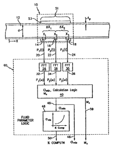
Referring to Fig. 1, a pipe (or conduit) 12 has three acoustic pressure
sensors
14,16,18, located at three locations x1,x2,x3 along the pipe 12. The pressure
may be
measured through holes in the pipe 12 ported to external pressure sensors or
by other
techniques discussed hereinafter. The pressure sensors 14,16,18 provide
pressure
time-varying signals Pi(t),P2(t),P3(t) on lines 20,22,24, to known Fast
Fourier
Transform (FFT) logics 26,28,30, respectively. The FFT logics 26,28,30
calculate
the Fourier transform of the time-based input signals Pl(t),P2(t), P3(t) and
provide
complex frequency domain (or frequency based) signals Pj(o)),P2(a),P3(w) on
lines
32,34,36 indicative of the frequency content of the input signals. Instead of
FFT's,
any other technique for obtaining the frequency domain characteristics of the
signals
P1(t),PZ(t),P3(t), may be used. For example, the cross-spectral density and
the power
spectral density may be used to form a frequency domain transfer functions (or
frequency response or ratios) discussed hereinafter.
-8-
CA 02335457 2007-01-18
Also, some or all of the functions within the logic 60 may be implemented in
software (using a microprocessor or computer) and/or firmware, or may be
implemented using analog and/or digital hardware, having sufficient memory,
interfaces, and capacity to perform the functions described herein.
The frequency signals P1(w),P2(ci)),P3((o) are fed to ami),-Mx Calculation
Logic
40 which provides a signal on a line 46 indicative of the speed of sound of
the
mixture ami,, (discussed more hereinafter). The am;,, signal is provided to
map (or
equation) logic 48, which converts am;, to a percent composition of the fluid
and
provides a %Comp signal on a line 50 indicative thereof (as discussed
hereinafter).
Also, if the Mach number Mx is not negligible and is desired to be known, the
calculation logic 40 may also provide a signal Mx on a line 59 indicative of
the Mach
number Mx (as discussed hereinafter).
More specifically, for planar one-dimensional acoustic waves in a
homogenous mixture, it is known that the acoustic pressure field P(x,t) at a
location
x along a pipe, where the wavelength X of the acoustic waves to be measured is
long
compared to the diameter d of the pipe 12 (i.e., ?Jd I), may be expressed as
a
superposition of a right traveling wave and a left traveling wave, as follows:
P(x, i) = (Ae -'k'X + Be +ikIx ian Eq. 1
where A,B are the frequency-based complex amplitudes of the right and left
traveling waves, respectively, x is the pressure measurement location along a
pipe, w
is frequency (in rad/sec, where w=2nf), and kr,ki are wave numbers for the
right and
left travelling waves, respectively, which are defrned as:
k,- =~ 1 and kl _ ty 1 Eq. 2
1+ M,
where am;,, is the speed of sound of the mixture in the pipe, co is frequency
(in
rad/sec), and Mx is the axial Macb number of the flow of the nzixture within
the pipe,
where: Mx = ymiX Eq. 3
amix
where Vmix is the axial velocity of the mixture. For non-homogenous mixtures,
the
-9-
CA 02335457 2007-01-18
axial Mach number represents the average velocity of the mixture and the low
frequency acoustic field description remains substantially unaltered.
The frequency domain representation P(x,co) of the time-based acoustic
pressure field P(x,t) within a pipe, is the coefficient of the e" ' term of
Eq. 1, as
follows:
P(x, cv) = Ae'kX + Be+'kjX Eq. 4
Referring to Fig. 1, we have found that using Eq. 4 for P(x,co) at three
axially
distributed pressure measurement locations xl,x2,x3 along the pipe 12 leads to
an
equation for amix as a function of the ratio of frequency based pressure
measurements,
which allows the coefficients A,B to be eliminated. For optimal results, A and
B are
substantially constant over the measurement time and substantially no sound
(or
acoustic energy) is created or destroyed in the measurement section. The
acoustic
excitation enters the test section only through the ends of the test section
51 and, thus,
the speed of sound within the test section 51 can be measured independent of
the
acoustic environment outside of the test section: In particular, the frequency
domain
pressure measurements PI (w),P2(w),P3(co) at the three locations xI,x2,x3,
respectively,
along the pipe 12 using Eq. I for right and left traveling waves are as
follows:
PI(co) =P(x = xl,uo) = Ae "k=s' +Be+'k's' Eq. 5
P2(w) = P(x = x2, tv) = Ae 'k'x2 + Be+,xlx2 Eq. 6
P3(c)) =P(x = x3,uo) = Ae 1kx' +Be+'k;' Eq. 7
where, for a given frequency, A and B are arbitrary constants describing the
acoustic
field between the sensors 14,16,18. Forming the ratio of Pj(w)/P2(co) from
Eqns.
6,7, and solving for B/A, gives the following expression:
e-fkA _ P1(6)) e=ik.xz
R=B= P~(CWO) Eq.8
A P ((w) le&,si - e&1X1
P2(t0)
where R is defined as the reflection coefficient.
Forming the ratio of P i(w)/P3(w) from Eqs. 5 and 7 and solving for zero
gives:
-10-
CA 02335457 2007-01-18
e-Tk's' + Re'k'r' P (tv)
= 0 Eq. 9
e-k,"' + Re'"'' ' ~ P3 (w)
where R=B/A is defined by Eq. 8 and kr and ki are related to am;., as defined
by Eq. 2.
Eq. 9 may be solved numerically, for example, by defining an "error" or
residual term
as the magnitude of the left side of Eq.9, and iterating to minimize the error
term.
I e 'k'X' + Re'k'F' _ P w
mag e'k'X' + Re'k'F' P3 (w) Error Eq. 10
For many applications in the oil industry, the axial velocity of the flow in
the
pipe is small compared to the speed of sound in the mixture (i.e., the axial
Mach
number M,, is small compared to one). For example, the axial velocity of the
oil V,;,
in a typical oil well is about 10 ft/sec and the speed of sound of oil aoij is
about 4,000
ft/sec. Thus, the Mach number Mx of a pure oil mixture is 0.0025
(Vo;Vaa;i=10/4,000), and Eq. 2 reduces to approximately:
kr = k, = W Eq. 11
a,,,;:
and the distinction between the wave numbers for the right and left traveling
waves
is eliminated. In that case (where Mx is negligible), since all of the
variables in Eq.
10 are known except for ami,,, the value for am;,, can be iteratively
determined by
evaluating the error term at a given frequency w and varying ami,, until the
error term
goes to zero. The value of am;,, at which the magnitude of the error term
equals zero
(or is a minimum), corresponds to the correct value of the speed of sound of
the
mixture amk. As Eq. 10 is a function of frequency w, the speed of sound am;"
at
which the error goes to zero is the same for each frequency w evaluated
(discussed
more hereinafter). However, in practice, there may be some variation over
certain
frequencies due to other effects, e.g., pipe modes, non-acoustical pressure
perturbation, discretization errors, etc., which may be filtered, windowed,
averaged,
etc. if desired (discussed more hereinafter). Furthermore, since each
frequency is an
independent measurement of the same parameter, the multiple measurements may
be weighted averaged or filtered to provide a single more robust measurement
of the
speed of sound.
-11-
CA 02335457 2007-01-18
One example of how the speed of sdund of the mixture amix in the pipe 12
may be used is to determine the volume fraction of the mixture. In particular,
the
speed of sound of a mixture amix of two fluids (where a fluid is defined
herein as a
liquid or a gas) in a pipe is in general related to the volume fraction of the
two
fluids. This relationship may be determined experimentally or analytically.
For
example, the speed of sound of a mixture may be expressed as follows:
F~aP2 amrx = I Eq. 12
aZ
Z
where aj,aZ are the known speeds of sound, p1,p2 are the known densities, and
hj,h2
are the volume fractions of the two respective fluids, am;x is the speed of
sound of the
mixture, and the densities p1,p2 of the two fluids are within about an order
of
magnitude (10:1) of each other. Other expressions relating the phase fraction
to
speed of sound may be used, being derived experimentally, analytically, or
computationally.
Referring to Fig. 2, where the fluid is an oil/water mixture, a curve 10 shows
the speed of sound of the mixture amix plotted as a function of water volume
fraction
using Eq. 12. For this illustrative example, the values used for density (p)
and speed
of sound (a) of oil and water are as follows:
Density (p): P Wat,= 1,000 kg/m3; Poii = 700 kg/m3
Speed of sound (a): a,~,~ = 5,000 fft/sec; aoij = 4,000 ft/sec.
The subscripts 1,2 of Eq. 12 assigned to the parameters for each fluid is
arbitrary
provided the notation used is consistent. Thus, if the speed of sound of the
mixture
amix is measured, the oillwater fraction may be determined.
Referring to Fig. 3, to illustrate the concept by example, a transmission
matrix model for the acoustics of an example pipe having 9 sections (or
elements or
segments) 1-9, an acoustic source 64, a radiation (or transmission) impedance
~,d
(~.e = P/pmixamixpmix) where m,x is an acoustic perhuba6on; Mx=O, and where
the
pressures P1,P2,P3 are measured across test sections 5-6 and 6-7. For this
example,
each elernent is I meter long.
-12-
CA 02335457 2007-01-18
Depending on the application, an explicit acoustic noise source may or may
not be required, as the background acoustic noises within the pipe may provide
sufficient excitation to enable a speed of sound measurement from existing
ambient
acoustic pressures. In an oil or gas well application, if the background
acoustic
noises are not sufficient, an acoustic noise source (not shown) may be placed
at the
surface of the well or within the well, provided the source is acoustically
coupled to
the test section 51 over which the speed of sound is measured.
Referring to Fig. 4, illustrations (a)-(c), an example of the axial properties
of
the mixture in the segments 1-9 of the pipe 12 is shown. The volume fraction
of
water h, the speed of sound of the mixture ami,,, and the density of the
mixture p,,,iX
vary over the length of the pipe 12 and the test segments 5,6 (from 4-6
meters)
between the pressure measurements PI-P3 have constant properties. In
particular, the
values for pmi,,, amix, hwata for sections 1-9, respectively, are shown
graphically in
Fig. 4 and are as follows:
hwacer = 0.1, 0.2, 0.3, 0.4, 0.5, 0.6, 0.7, 0.8, 0.9;
pmiX = 730, 760, 790, 820, 850, 850, 910, 940, 970 (kg/m3);
an,i,, = 4053, 4111, 4177, 4251, 4334, 4334, 4539, 4667, 4818 (ft/sec);
Referring to Figs. 5,6, the magnitude and phase of the ratio of the frequency
based pressure signals P1(w)/P2((0) and Pi(w)/P3((6) is shown for the model of
Fig. 3
with the properties of Fig. 4 with 50% water in the test section and a
radiation
impedance of ~rad = 1.0 corresponding to an infinitely long pipe with constant
properties of pm;,, and ami,, for section 9 and beyond.
Referring to Fig. 7, the error term of Eq. 10 using the frequency responses of
Figs. 5,6, is a faniily of curves, one curve for each frequency w, where the
value of
the error is evaluated for values of amiX varied from a"at.' (5,000 ft/sec) to
a;j (4,000
ft/sec) at each frequency and the frequency is varied from 5 to 200 Hz in 5 Hz
increments. Other frequencies may be used if desired. The speed of sound
aõoi,, where
the error goes to zero (or is minimized) is the same for each frequency co
evaluated.
In this case, the error is minimized at a point 70 when am;., is 4335 fdsec.
From Fig.
2, for an oil/water mixture, an ami,, of 4335 ft/sec corresponds to a 50%
water
volume ratio in the test section which matches the water fraction of the
model.
.
-13-
CA 02335457 2007-01-18
Also, the sensitivity of a change in a,,,;X to a change in error varies based
on the
evaluation frequency. Thus, the performance may be optimized by evaluating
am;, at
specific low sensitivity frequencies, such frequencies to be determined
depending on
the specific application and configuration.
Referring to Figs. 8,9, for an radiation impedance i;rad = 0.5, the magnitude
and phase of the frequency responses (i.e., the ratio of frequency based
pressure
signals) Pi((O)/P2(co) and P1((O)/P3(0)) is shown for the model of Fig. 3 with
constant
properties across all sections 1-9 of 50% water fraction (h=0.5), density of
mixture
pm;x 850 kg/m3, and speed of sound of mixture amiX 4334 ft/sec.
Referring to Fig. 12, for a 50% water fraction, the magnitude of the error
tcrm of Eq. 10 using the frequency responses of Figs. 8,9, is a family of
curves, one
curve for each frequency w, where the value of aR,ix is varied from a,,,,a,,
(5,000
ft/sec) to aoil (4,000 ft/sec) at each frequency and is shown at four
frequencies
50,100,150,200 Hz. As discussed hereinbefore, the speed of sound am;,, where
the
error goes to zero (or is minimized) is the same for each frequency co
evaluated. In
this case, the error is minimized at a point 72 where am;X = 4334 ft/sec,
which
matches the value of ami,, shown in Fig. 7 for the same water fraction and
different
~rad. From Fig. 2 (or Eq. 2), for an oil/water mixture, an amiX of 4334 fl/sec
.corresponds to a 50% water volume ratio in the test section which corresponds
to the
water fraction of the model. This shows that the invention will accurately
determine
ami,, independent of the acoustic properties of the mixture outside the test
sections
and/or the ternunation impedances.
Referring to Figs. 10,11, the magnitude and phase of the frequency responses
(i.e., the ratio of the frequency based pressure signals) Pi((O)/P2((u) and
Pi(W)1P3((O)
is shown for the model of Fig. 3 with constant properties across all sections
1-9 of
5% water fraction (h=0.05), density of mixture p~,u 715 kg/m3, and speed of
sound
of mixture am;x 4026 fft/sec, and a radiation impedance C,rad = 0.5.
Referring to Fig. 12, for a 5% water fraction, the magnitude of the error term
of Eq. 10 using the frequency responses of Figs. 10,11, is a family of dashed
curves,
one curve for each frequency W, where the value of a;x is varied from a,yAa
(5,000
ft/sec) to aoil (4,000 ft/sec).at each frequency and is shown at four
frequencies
-14-
CA 02335457 2007-01-18
50,100,150,200 Hz. As discussed hereinbefore, the speed of sound am;X where
the
error goes to zero (or is minimized) is the same for each frequency w
evaluated. In
this case, the error is minimized at a point 74 when am;,' = 4026 fl/sec. From
Fig. I
(or Eq. 1), for an oil/water mixture, an am;,, of 4026 ft/sec corresponds to a
5% water
volume ratio in the test section which corresponds to the water fraction of
the model
and, thus, verifies the results of the model.
Referring to Fig. 12, for both 5% and 50% water fraction, the sensitivity of a
change in am;,, to a change in error varies based on the evaluation frequency.
In
particular, for this example, of the four frequencies shown, the error
approaches zero
with the largest slope (DError/Dam;,,) for the 200 Hz curve, thereby making it
easier
to detect the value whcrc the error goes to zero, and thus the value of
a,,,;x. Thus, 200
Hz would likely be a robust frequency to use to determine the speed of sound
in this
example.
If the pressure sensors are equally spaced (i.e., xl-x2 = x3-x2 = Ax; or
Ax1=0x2=Ax) and the axial Mach number Mx is small compared to one (and thus,
kr=kl=k), Eq. 10 may be solved for k (and thus ami,, ) in a closed-form
solution as a
function of the pressure frequency responses (or frequency based signal
ratios) as
follows:
~z
k=~ = f1li Pz + P3P,Z + Pi2 + 2P13P122 + P13' P12Z - 4P132 13
L~J log 2P13 Eq.
amix
Solving for am;,,, gives:
El
a _
~ 1 i1091 P2 + P3P2 +(PZZ + w 2P;P22 +PjZPZ2 -4P32)~~2 1
~~~ 2Pis
where P12 =P1(w)/P2(W), P13=P1(w)/P3(0), i is the square root of-1, and the
result
of the Log[] function is an imaginary number, yielding a real number for the
speed
of sound amiX.
The analytical solution to the Eq. 10 shown in Eqs. 13 and 14 is valid
primarily for the frequencies for which the length of the test section 51
along the
pipe 12 (i.e., x3-x 1 or 2Ax for equally spaced sensors) is shorter than the
wavelength
-15-
CA 02335457 2007-01-18
X of the acoustic waves to be measured. This restriction is due to multiple
possible
solutions to the Eq. 10. Alternative solutions to Eq. 10 for other frequency
ranges
may be derived using a variety of known techniques.
An altetnative closed form solution for am;X (in a trigonometric form) from
the three pressure Eqs. 5-7, where the pressure sensors are equally spaced and
Mx is
negligible (i.e, kl=kr), is as follows. Forming the ratio [Pt(w) +
P3(cw)J/P2((O) from
Eqs. 5-7, gives the following expression:
P(w) + P3 (w) Ae-'""' + Be+"b' + Ae-'kr' + Be+'kr'
E IS
1'2 (~) Ae-'kx2 + Be+kxz q
For equally spaced sensors, x1=0,x2=Ax, x3=2Ax (x1=0 for convenience
only), which gives:
P,(cv)+P3(w) _ A+B+Ae-2ikAx +Be+2kGx
P2 (CO) Ae-''' x + Be+'k x Eq. 16
Dividing the numerator and denominator by A, gives:
P,(w)+P3(tv) _ 1+R+e -2ikdz +Re +2ikAx
P2 (0)) e-'k x + Re+k x Eq. 17
where R=B/A is defmed by Eq. 8 with x1=0,x2=ex, which gives:
1 _ Pi (w } e-rkex
B ~'2(w)
R A~, IC0)le1_i
P2(w)
Plugging R into Eq. 17, gives:
1 _ Pi (co) ]e-a6'
l+e'2ikAx + P2(CO) +(1+e+2irax)
FlP (w) e''r'ex -1
P,(W)+P3(u~) 1'2(CO)
P2 (w) 1_ P(O)) e-ikv Eq. 19
e-iknx + P2 (0)) e+ike:
Pi (w) le-i
~'2(w)
-16-
CA 02335457 2007-01-18
Simplifying Eq. 19, gives:
(P2 e+i,~er _ 1(I + ePe-'"" (1 + e+2;-~ex P(t)) + P, (<v) _ z J
Eq.
P2 (w) e+u~eX _ 1(e '"' x )+ 1- P e-,~ (e,.i~l Eq
F'z PZ 1
Distributing terms and simplifying, gives:
P(~v)+P3 (tc~) -e 2i~ " +e+2-kex
5 P2 (w} - e-,r& + e+,xer Eq. 21
Using the relation between exponents and the sine function, gives:
P, (co) + P(tv) 2i sin(2k&z) 2 sin(kx) cos(kx)
PZ (tr~) 2i sin(kx) sin(kx) Eq. 22
Simplifying and substituting k=co/am;,,, gives:
P, (Cy) + P3 (aO) _ 2 cos(kAx) = 2 co Eq. 23
P2 (CO) amix
10 Eq. 23 is particularly useful due to its simple geometric form, from which
amix can be easily interpreted. In particular, am;,, can be determined
directly by
inspection from a digital signal analyzer (or other similar instrument) set up
to
provide a display indicative of the left side of Eq. 23, which will be a
cosine curve
from which amiX may be readily obtained. For example, at the zero crossing of
the
15 cosine wave, Eq. 23 will be equal to zero and a;x will be equal to 2coOX/n.
Alternatively, Eq. 23 may be used to determine amix using an iterative
approach
where a measured function is calculated from the left side of Eq. 23 (using
the
measured pressures) and compared to a cosine curve of the right side of Eq. 23
where amix is varied until it substantially matches the measured function.
Various
20 other curve fitting, parameter identification, and/or minimum error or
solution
techniques may be used to deternune the value of amix that provides the best
fit to
satisfy Eq. 23.
Solving Eq. 23 for aR,;,,, gives the following closed-form solution:
-17-
CA 02335457 2007-01-18
wOaC Q1dx
amix Eq. 24
COS I (PI (c)) + P3 (01) COS I 1 P(lO) + P3 (L~)
2P2 (co) 2 P2 (w) P2 (w)
Referring to Fig. 41, a graph of speed of sound (am;,,) versus water cut is
shown where am;, is calculated using Eq. 23 as described hereinbefore. Fig. 41
is for
a Schedule 160 steel pipe having a 2 inch ID, AX=2ft even spacing between
three
axial sensing.locations, each sensor being a piezo-electric ac pressure
sensor, there
being four evenly circumferentially spaced sensors at each axial sensing
location.
The line 452 shows the theoretical value for water cut based on Eq.12 and Fig.
2
discussed hereinbefore, and the circles are the calculated values for am;X.
Alternatively, Eq. 9 may be written in trigonometric form for arbitrary
spacing
between the pressure sensors and where Mx is negligible (kl=kr), as follows:
si (x3 - x, ) - P32 si (x2 - x, ) - PZ si co (x3 - x2 ) = 0 Eq. 25
amix amix amiuc
where P32 = P3(0))/P2((o) and P12 = P1(C0)/P2(0)).
Refen=ing to Figs. 13,14, if Mach number Mx is not negligible and/or is
desired to be calculated, the value of Mx and aR,;,, where the error term of
Eq. 10 is
zero can be uniquely determined from Eq. 10 for a given water fraction. In
particular, for a given %water fraction, there is a unique value indicated by
points
90,92 for 5%. and 50% water cut, respectively. Known software search
algorithms
may be used to vary amk and Mx over predetermined ranges to find the value of
Mx
and amk where the error = 0(discussed more hereinafter).
Referring to Fig. 15, the calculation logic 40 begins at a step 100 where P12
is calculated as the ratio of PE(w)/P2(ow), and a step 102 whereP13 is
calculated as the
ratio of P1((6)/P3(W). Next a step 103 deterniines whether the Mach number Mx
of
the mixture is negligible (or whether it is desirable to calculate Mx). If Mx
is
negligible, a step 104 determines if the sensors 14,16,18 are equally spaced
(i.e., x 1-
x2=x2-x3=0x). If equally spaced sensors, steps 106 set initial values for w=
w1
(e.g., 100 Hz) and a counter n=1. Next, a step 108 calculates am;,,(n) from
the closed
form solution of Eq. 14. Then, a step 110 checks whether the logic 40 has
calculated a,,;x at a predetermined number of frequencies, e.g., 10. If n is
not greater
-18-
CA 02335457 2007-01-18
than 10, steps 112,114, increments the counter n by one and increases the
frequency
cu by a predetermined amount (e.g., 10 Hz) and the step 108 is repeated. If
the logic
40 has calculated amix at 10 frequencies, the result of the step 116 would be
yes and
the logic 40 goes to a step 116 which determines an average value for amix
using the
~ 5 values of am;x(n) over the 10 frequencies, and the logic 40 exits.
If the sensors are not equally spaced, steps 120 set xl,x2,x3 to the current
pressure sensor spacing, and set initial values for w= wl (e.g., 100 Hz) and
the
counter n=1. Next, a step 122 sets amix= amtx_m;,, (e.g., ao;f=4000 ft/sec)
and a step 124
calculates the error term from Eq. 10. Then, a step 126 checks whether error =
0. If
the error does not equal zero, a;x is incremented by a predetermined amount
and the
logic 40 goes to a step 124.
If the error=0 (or a minimum) in step 126, a step 130 sets am;x(n) =amix.
Next,
a step 132 checks whether n is greater than or equal to 10. If not, a step 134
increments n by one and increases the frequency co by a predetermined amount
(e.g.,
10 Hz). If n is greater than or equal to 10, a step 138 calculates an average
value for
am;x over the 10 frequencies.
Referring to Fig. 16, if the Mach number Mx is not negligible, steps 200-204
sets initial conditions: w=(@ 1(e.g., 100 Hz); Mx-Mx-min (e.g., 0); am;x amix-
min (e.g.,
4it=4000 ft/sec). Then, a step 206 calculates the error term of Eq. 10 at a
step 202.
Next, a step 208 checks whether the error=0 (or a minimum). If not, a step 210
checks whether am;X amix-max (e.g., awater 5000 ft/sec).
If the result of step 210 is no, a step 212 increases amu by a predetermined
amount (e.g., I ft/sec) and the logic goes to step 206. If the result of step
210 is yes,
a step 214 increases Mx by a predetermined amount (e.g., 1) and the logic goes
to
step 204.
When step 208 indicates error=0 (or a minimum), a step 216 sets an,ix(n)=am;.
and Mx(n)=Mx, and a step 218 checks whether the values of a,,,;,, and Mx have
been
calculated at 10 different frequencies. If not, a step 220 increments the
counter n by
one and a step 222 increases the value of the frequency co by a predetermined
amount (e.g., 10 Hz). If the values of am;x and Mx have been calculated at 10
different frequencies (i.e., n is equal to 10), a step 224 calculates a
average values
-19-
CA 02335457 2007-01-18
for am;,,(n) and Mx(n) at the 10 different frequencies to calculate am;x and
Mx. The
value for amix above is similar to that shown in Figs. 13,14, discussed
hereinbefore,
where the final value of am;,, are the points 90,92 where the error equals
zero.
Instead of calculating an average value for amix in steps 116,138,24, am;,,
may
be calculated by filtering or windowing am;x(n), from predetermined
frequencies.
The number of frequencies and the frequencies evaluated may be any desired
number and values. Also, instead of calculating an,;,, and/or Mx at more than
one
frequency, it may be calculated at only one frequency. Further, the logic
shown in
Figs. 15,16 is one of many possible algorithms to calculate amix using the
teachings
herein.
Refening to Figs. I and 18, the compliance (or flexibility) of the pipe 12 (or
conduit) in the sensing region may influence the accuracy or interpretation of
the
measured speed of sound ami,, of the mixture in two primary, ways.
Regarding the first way, referring to Fig. 18, flexing of the pipe 12 in the
sensing region reduces the measured speed of sound aR,;X from the sound in an
unbounded domain. The sound speed in an unbounded domain (infinite media) is a
property that is closely linked with the fluid properties. In particular, the
influence
of pipe wall thickness (or compliance of the pipe) on measured speed of sound
due
reduction in the speed of sound for a pipe having a 2 inch nominal diameter
and
having 100% water (pW=1,000 kg/m3; aw=5,000 ft/see) inside the pipe and a
vacuum
(or air) outside the pipe diameter, is shown. The speed of sound of water in
an
infinitely rigid pipe (i.e., infinite modulus) is indicated by a flat curve
350, and the
speed of sound of water in a steel pipe is indicated by a curve 352. A point
354 on
the curve 352 indicates the value of the speed of sound of about 4768 ft/sec
for a
Schedule 80 steel pipe. Accordingly, the thicker the pipe wall, the closer the
speed
of sound approaches the value of 5,000 ft/sec for an infinitely rigid pipe.
The errors (or boundary effects) shown in Fig. 18 introduced into the
measurements by a non-rigid (or compliant) pipe 12 can be calibrated and
corrected
for to accurately determine the speed of sound in the fluid in an unbounded
media.
Thus, in this case, while the system (pipe) does modify the propagation
velocity,
-20-
CA 02335457 2007-01-18
such velocity can be mapped to the propagation velocity in an infinite media
in a
predictable fashion.
In particular, for fluids contained in a compliant pipe, the propagation
velocity of compression waves is influenced by the structural properties of
the pipe.
For a fluid contained in the pipe 12 surrounded witha fluid of negligible
acoustic
impedance (pa), the propagation velocity is related to the infinite fluid
domain speed
of sound and the structural properties via the following relation:
2 = 12 + ar where 6 Et Eq.26
P,õ;.a inea,sured P.u a,nis
where R= the pipe radius, t is the pipe wall thickness, pm;,, is the density
of
the mixture (or fluid), a;., is the actual speed of sound 'of the mixture,
ai11e,,,õTed is the
measured speed of sound of the mixture contained in the pipe 12, and E is the
Young's modulus for the pipe material. Eq. 26 holds primarily for frequencies
where the wavelength of the acoustics is long (e.g., greater than about 2 to
1)
compared to the diameter of the pipe and for frequencies which are low
compared to
the natural frequency of the breathing mode of the pipe. Eq. 26 also applies
primarily to wavelengths which are long enough such that hoop stiffness
dominates
the radial deflections of the pipe.
For Fig. 18, the curve 352 (for 100% water) would be one of a family of
curves for various different oiUwater mixtures. For Eq. 26, the terms may be
defined
in terms of the density of each constituent, and the volumetric phase fraction
as
follows:
12 = ~ ~r 2 where: . Pu,rx ~rP; and 0; =1
PMUa i. M Pra, s=i r=i
where p; is the density of the id' constituent of a multi-component mixture,
aF
is the sound speed of the ite constituent of the mixture, ~; is the volumetric
phase
fraction of the i'h constituent of the mixture, and N is the number of
components of
the mixture_ Knowing the pipe properties, the densities and the sound speed
(in an
infinite domain) of the individual constituents, and the measured sound speed
of the
mixture, Eq. 26 can be solved for ami,,. Thus, amix can be determined for a
compliant
-21-
CA 02335457 2007-01-18
pipe. The calibration of the pipe can be derived from other equations or from
a
variety of other means, such as analytical, experimental, or computational.
For certain types of pressure sensors, e.g., pipe strain sensors,
accelerometers, velocity sensors or displacement sensors, discussed
hereinafter, it
may be desirable for the pipe 12 to exhibit a certain amount of pipe
compliance.
Alternatively, to minimize these error effects (and the need for the
corresponding calibration) caused by pipe compliance, the axial test section
51 of
the pipe 12 along where the sensors 14,16,18 are located may be made as rigid
as
possible. To achieve the desired rigidity, the thickness of the wall 53 of the
test
section 51 may be made to have a predetermined thickness, or the test section
51
may be made of a very rigid material, e.g., steel, titanium, Kevlar , ceramic,
or other
material with a high modulus.
Regarding the second way, if the pipe 12 is compliant and acoustically
coupled to fluids and materials outside the pipe 12 in the sensing region,
such as the
annulus fluid, casing, rock formations, etc., the acoustic properties of these
fluids
and materials outside the pipe 12 diameter may influence the measured speed of
sound. Because the acoustic properties of such fluids and materials are
variable and
unknown, their affect on measured speed of sound cannot be robustly corrected
by
calibration (nor mapped to the propagation velocity in an infinite media in a
predictable fashion).
Referring to Fig. 20, to alleviate this effect, an outer isolation sleeve 410
(or
sheath, shell, housing, or cover) which is attached to the outer surface of
pipe 12
over where the pressure sensors 14,16,18 are located on the pipe 12. The
sleeve 410
forms a closed chamber 412 between the pipe 12 and the sleeve 410. We have
found
that when the chamber 412 is filled with a gas such as air, the acoustic
energy in the
pipe is not acoustically coupled to fluids and materials outside the pipe 12
in the
sensing region. As such, for a compliant pipe the speed of sound can be
calibrated to
the actual speed of sound in the fluid in the pipe 12 as discussed
hereinbefore. The
sleeve 410 is similar to that disclosed in U.S. 6,435,030, entitled
"Measurement of
Propagating Acoustic Waves in Compliant Pipes".
-22-
CA 02335457 2007-01-18
Referring to Fig. 19, instead of single point pressure sensors 14,16,18, at
the
axial locations xl,x2,x3 along the pipe 12, two or more pressure sensors,
e.g., four
sensors 400-406, may be used around the circumference of the pipe 12 at each
of the
axial locations xl,x2,x3. The signals from the pressure sensors 400-406 around
the
circumference at a given axial location may be averaged to provide a cross-
sectional
(or circumference) averaged unsteady acoustic pressure measurement. Other
numbers of acoustic pressure sensors and annular spacing may be used.
Averaging
multiple annular pressure sensors reduces noises from disturbances and pipe
vibrations and other sources of noise not related to the one-dimensional
acoustic
pressure waves in the pipe 12, thereby creating a spatial array of pressure
sensors to
help characterize the one-dimensional sound field within the pipe 12.
The pressure sensors 14,16,18 described herein may be any type of pressure
sensor, capable of measuring the unsteady (or ac or dynamic ) pressures within
a
pipe, such as piezoelectric, optical, capacitive, resistive (e.g., Wheatstone
bridge),
accelerometers (or geophones), velocity measuring devices, displacement
measuring
devices, etc. If optical pressure sensors are used, the sensors 14-18 may be
Bragg
grating based pressure sensors, such as that described in US Patent
6,016,702 entitled "High Sensitivity Fiber Optic Pressure
Sensor For Use In Harsh Environments", filed Sept. 8, 1997. Alternatively, the
sensors 14-18 may be electrical or optical strain gages attached to or
embedded in
the outer or inner wall of the pipe which measure pipe wall strain, including
microphones, hydrophones, or any other sensor capable of measuring the
unsteady
pressures within the pipe 12. In an embodiment of the present invention that
utilizes
fiber optics as the pressure sensors 14-18, they may be connected individually
or
may be multiplexed along one or more optical fibers using wavelength division
multiplexing (WDM), time division multiplexing (TDM), or any other optical
multiplexing techniques (discussed more hereinafter).
Referring to Fig. 21, if a strain gage is used as one or more of the pressure
sensors 14-18, it may measure the unsteady (or dynamic or ac) pressure
variations
Pin inside the pipe 12 by measuring the elastic expansion and contraction, as
represented by arrows 350, of the diameter (and thus the circumference as
-23-
CA 02335457 2007-01-18
represented by arrows 351) of the pipe 12. In general, the strain gages would
measure the pipe wall deflection in any direction in response to unsteady
pressure
signals inside the pipe 12. The elastic expansion and contraction of pipe 12
is
measured at the location of the strain gage as the internal pressure Pin
changes, and
thus measures the local strain (axial strain, hoop strain or off axis strain),
caused by
deflections in the directions indicated by arrows 351, on the pipe 12. The
amount of
change in the circumference is variously determined by the hoop strength of
the pipe
12, the internal pressure Pi,,, the external pressure Poõt outside the pipe
12, the
thickness Ta, of the pipe wall 352, and the rigidity or iriodulus of the pipe
material.
Thus, the thickness of the pipe wal1352 and the pipe material in the sensor
sections
51 (Fig. 1) may be set based on the desired sensitivity of sensors 14-18 and
other
factors and may be different from the wall thickness or material of the pipe
12
outside the sensing region 51.
Still with reference to Fig. 21 and Fig. 1, if an accelerometer is used as one
or more of the pressure sensors 14-18, it may measure the unsteady (or dynamic
or
ac) pressure variations Pin inside the pipe 12 by measuring the acceleration
of the
surface of pipe 12 in a radial direction, as represented by arrows 350. The
acceleration of the surface of pipe 12 is measured at the location of the
accelerometer as the internal pressure Piõ changes and thus measures the local
elastic
dynamic radial response of the wall 352 of the pipe. The magnitude of the
acceleration is variously determined by the hoop strength of the pipe 12, the
internal
pressure P;,,, the external pressure Pou, outside the pipe 12, the thickness
Tw of the
pipe wall 352, and the rigidity or modulus of the pipe material. Thus, the
thickness
of the pipe wall 352 and the pipe material in the sensing section 51 (Fig. 1)
may be
set based on the desired sensitivity of sensors 14-18 and other factors and
may be
different from the wall thickness or material of the pipe 12 outside the
sensing
region 14. Alternatively, the pressure sensors 14-18 may comprise a radial
velocity
or displacement measurement device capable of measuring the radial
displacement
characteristics of wall 352 of pipe 12 in response to pressure changes caused
by
unsteady pressure signals in the pipe 12. The accelerometer, velocity or
displacement sensors may be similar to those described in commonly-owined
-24-
CA 02335457 2007-01-18
US Patent 6,463,813 entitled "Displacement Based Pressure Sensor Measuring
Unsteady
Pressure in a Pipe".
Referring to Figs. 22,23,24, if an optical strain gage is used, the ac
pressure
sensors 14-18 may be configured using an optical fiber 300 that is coiled or
wrapped
around and attached to the pipe 12 at each of the pressure sensor locations as
indicated by the coils or wraps 302,304,306 for the pressures Pt,P2,P3,
respectively.
The fiber wraps 302-306 are wrapped around the pipe 12 such that the length of
each of the fiber wraps 302-306 changes with changes in the pipe hoo_p strain
in
response to unsteady pressure variations within the pipe 12 and thus internal
pipe
pressure is measured at the respective axial location. Such fiber length
changes are
measured using known optical measurement techniques as discussed hereinafter.
Each of the wraps measure substantially the circumferentially averaged
pressure
within the pipe 12 at a corresponding axial location on the pipe 12. Also, the
wraps
provide axially averaged pressure over the axial length of a given wrap. While
the
structure of the pipe 12 provides some spatial filtering of short wavelength
disturbances, we have found that the basic principle of operation of the
invention
remains substantially the same as that for the point sensors described
hereinbefore.
Referring to Fig. 22, for embodiments of the present invention where the
wraps 302,304,306 are connected in series, pairs of Bragg gratings
(310,312),(314,316), (318,320) may be located along the fiber 300 at opposite
ends
of each of the wraps 302,304,306, respectively. The grating pairs are used to
multiplex the pressure signals P1iP2,P3 to identify the individual wraps from
optical
return signals. The first pair of gratings 310,312 around the wrap 302 may
have a
common reflection wavelength Xi, and the second pair of gratings 314,316
around
the wrap 304 may have a common reflection wavelength X2, but different from
that
of the first pair of gratings 310,312. Similarly, the third pair of gratings
318,320
around the wrap 306 have a common reflection wavelength X3, which is different
from kl,)L2.
Referring to Fig. 23, instead of having a different pair of reflection
wavelengths associated with each wrap, a series of Bragg gratings 360-366 with
-25-
CA 02335457 2007-01-18
only one grating between each of the wraps 302-306 may be used each having a
common reflection wavlength X1.
Referring to Figs. 22 and 23 the wraps 302-306 with the gratings 310-320
(Fig.22) or with the gratings 360-366 (Fig.23) may be configured in numerous
known ways to precisely measure the fiber length or change in fiber length,
such as
an interferometric, Fabry Perot, time-of-flight, or other known arrangements.
An
example of a Fabry Perot technique is described in US Patent. No. 4,950,883
"Fiber
Optic Sensor Arrangement Having Reflective Gratings Responsive to Particular
Wavelengths", to Glenn. One example of time-of-flight (or Time-Division-
Multiplexing; TDM) would be where an optical pulse having a wavelength is
launched down the fiber 300 and a series of optical pulses are reflected back
along
the fiber 300. The length of each wrap can then be determined by the time
delay
between each return pulse.
Alternatively, a portion or all of the fiber between the gratings (or
including
the gratings, or the entire fiber, if desired) may be doped with a rare earth
dopant
(such as erbium) to create a tunable fiber laser, such as is described in US
Patent No.
5,317,576, "Continuously Tunable Single Mode Rare-Earth Doped Laser
Arrangement", to Ball et al or US Patent No. 5,513,913, "Active Multipoint
Fiber
Laser Sensor", to Ball et al, or US Patent No. 5,564,832, "Birefringent Active
Fiber
Laser Sensor", to Ball et al. -
While the gratings 310-320 are shown oriented axially with respect to pipe
12, in Figs. 22,23, they may be oriented along the pipe 12 axially,
circumferentially,
or in any other orientations. Depending on the orientation, the grating may
measure
deformations in the pipe wa11352 with varying levels of sensitivity. If the
grating
reflection wavelength varies with intemal pressure changes, such variation may
be
desired for certain configurations (e.g., fiber lasers) or may be compensated
for in
the optical instrumentation for other configurations, e.g., by allowing for a
predetermined range in reflection wavelength shift for each pair of gratings.
Alternatively, instead of each of the wraps being connected in series, they
may be
connected in parallel, e.g., by using optical couplers (not shown) prior to
each of the
wraps, each coupled to the common fiber 300.
-26-
CA 02335457 2007-01-18
Referring to Fig. 24, alternatively, the sensors 14-18 may also be formed.as a
purely interferometric sensor by wrapping the pipe 12 with the wraps 302-306
without using Bragg gratings where separate fibers 330,332,334 may be fed to
the
separate wraps 302,304,306, respectively. In this particular embodiment, known
interferometric techniques may be used to detetmine the length or change in
length
of the fiber 10 around the pipe 12 due to pressure changes, such as Mach
Zehnder or
Michaelson Interferometric techniques, such as that described in US Patent
5,218,197, entitled "Method and Apparatus for the Non-invasive Measurement of
Pressure Inside Pipes Using a Fiber Optic Iriterferometer Sensor" to Carroll.
The
inteferometric wraps may be multiplexed such as is described in Dandridge, et
al,
"Fiber Optic Sensors for Navy Applications", IEEE, Feb. 1991, or Dandridge, et
al, .
"Multiplexed Intereferometric Fiber Sensor Arrays", SPIE, Vol. 1586, 199 1, pp
176-
183. Other techniques to determine the change in fiber length may be used.
Also,
reference optical coils (not shown) may be used for certain interferometric
approaches and may also be located on or around the pipe 12 but may be
designed to
be insensitive to pressure variations.
Referring to Figs. 25 and 26, instead of the wraps 302-306 being optical fiber
coils wrapped completely around the pipe 12, the wraps 302-306 may have
alternative geometries, such as a "radiator coil" geometry (Fig 25) or a "race-
track"
geometry (Fig. 26), which are shown in a side view as if the pipe 12 is cut
axially
and laid flat. In this particular embodiment, the wraps 302-206 are not
necessarily
wrapped 360 degrees around the pipe, but may be disposed over a predetermined
portion of the circumference of the pipe 12, and have a length long enough to
optically detect the changes to the pipe circumference. Other geometries for
the _
wraps may be used if desired. Also, for any geometry of the wraps described
herein,
more than one layer of fiber may be used depending on the overall fiber length
desired. The desired axial length of any particular wrap is set depending on
the
characteristics of the ac pressure desired to be measured, for example the
axial
length of the pressure disturbance caused by a vortex to be measured.
Referring to Figs. 27 and 28, embodiments of the present invention include
configurations wherein instead of using the wraps 302-306, the fiber 300 may
have
-27-
CA 02335457 2007-01-18
shorter sections that are disposed around at least a portion of the
circumference of
the pipe 12 that can optically detect changes to the pipe circumference. It is
further
within the scope of the present invention that sensors may comprise an optical
fiber
300 disposed in a helical pattern (not shown) about pipe 12. As discussed
herein
above, the orientation of the strain sensing element will vary the sensitivity
to
deflections in pipe wal1352 deforniations caused by unsteady pressure signals
in the
pipe 12.
Referring to Fig. 27, in particular, the pairs of Bragg gratings (310,312),
(314,316), (318,320) are located along the fiber 300 with sections 380-384 of
the
fiber 300 between each of the grating pairs, respectively. In that case, known
Fabry
Perot, inierferometric, time-of-flight or fiber laser sensing techniques may
be used to
measure the strain in the pipe, in a manner similar to that described in the
aforementioned references.
Referring. to Fig. 28, alternatively, individual gratings 370-374 may be
disposed on the pipe and used to sense the unsteady variations in strain in
the pipe
12 (and thus the unsteady pressure within the pipe) at the sensing locations.
When a
single grating is used per sensor, the grating reflection wavelength shift
will be
indicative of changes in pipe diameter and thus pressure.
Any other technique or configuration for an optical strain gage may be used.
The type of optical strain gage technique and optical signal analysis approach
is not
critical to the present invention, and the scope of the invention is not
intended to be
limited to any particular technique or approach.
For any of the embodiments described herein, the pressure sensors, including
electrical strain gages, optical fibers and/or gratings among others as
described
herein, may be attached to the pipe by adhesive, glue, epoxy, tape or other
suitable
attachment means to ensure suitable contact between the sensor and the pipe
12.
The sensors may alternatively be removable or permanently attached via known
mechanical techniques such as mechanical fastener, spring loaded, clamped,
clam
shell arrangement, strapping or other equivalents. Alternatively, the strain
gages,
including optical fibers and/or gratings, may be embedded in a composite pipe.
If
-28-
CA 02335457 2007-01-18
desired, for certain applications, the gratings may be detached from (or
strain or
acoustically isolated from) the pipe 12 if desired.
Referring to Figs. 29,30, it is also within the scope of the present invention
that any other strain sensing technique may be used to measure the variations
in
strain in the pipe, such as highly sensitive piezoelectric, electronic or
electric, strain
gages attached to or embedded in the pipe 12. Referring to Fig. 29, different
known
configurations of highly sensitive piezoelectric strain gages are shown and
may
comprise foil type gages. Referring to Fig. 30, an embodiment of the present
invention is shown wherein pressure sensors 14-18 comprise strain gages 320.
In
this particular embodiment strain gages 320 are disposed about a predetermined
portion of the circumference of pipe 12. The axial placement of and separation
distance AXI, AX2 between the pressure sensors 14-18 are determined as
described
herein above.
Referring to Figs. 31-33, instead of measuring the unsteady pressures PJ-P3
on the exterior of the pipe 12, the invention will also work when the unsteady
pressures are measured inside the pipe 12. In particular, the pressure sensors
14-18
that measure the pressures P0Z,P3 may be located anywhere within the pipe 12
and
any technique may be used to measure the unsteady pressures inside the pipe
12.
Referring to Figs. 34-36, the invention may also measure the speed of sound
of a mixture flowing outside a pipe or tube 425. In that case, the tube 425
may be
placed within the pipe 12 and the pressures P1-P3 measured at the outside of
the tube
425. Any technique may be used to measure the unsteady pressures Pl-P3 outside
the
tube 425. Referring to Fig. 34, for example, the tube 425 may have the optical
wraps
302-306 wrapped around the tube 425 at each sensing location. Alternatively,
any of
the strain measurement or displacement, velocity or accelerometer sensors or
techniques described herein may be used on the tube 425. Refen-ing to Fig. 35,
alternatively, the pressures P1-P3 may be. measured using direct pressure
measurement sensors or techniques described herein. Any other type of unsteady
pressure sensors 14-18 may be used to measure the unsteady pressures within
the
pipe 12.
-29-
CA 02335457 2007-01-18
Alternatively, referring to Fig. 36, hydrophones 430-434 may be used to
sense the unsteady pressures within the pipe 12. In that case, the hydrophones
430-
434 may be located in the tube 425 for ease of deployment or for other
reasons. The
hydrophones 430-434 may be fiber optic, electronic, piezoelectric or other
types of
hydrophones. If fiber optic hydrophones are used, the hydrophones 430-434 may
be
connected in series or parallel along the common optical fiber 300.
The tube 425 may be made of any material that allows the unsteady pressure
sensors to measure the pressures PI-P3 and may be hollow, solid, or gas filled
or
fluid filled. One example of a dynamic pressure sensor is described in
commonly-owned US Patent 6,233,374 entitled "Mandrel Wound Fiber Optic
Pressure Sensor",
filed June 4, 1999. Also, the end 422 of the tube 425 is closed and thus the
flow path would be
around the end 422 as indicated by lines 424. For oil and gas well
applications, the
tube 425 may be coiled tubing or equivalent deployment tool having the
pressure
sensors 14-18 for sensing Pt-P3 inside the tubing 425.
Referring to Fig. 17, there is shown an embodiment of the present invention
in an oil or gas well application, the sensing section 51 may be connected to
or part
of production tubing 502 (analogous to the pipe 12 in the test section 51)
within a
wel1500. The isolation sleeve 410 may be located over the sensors 14-18 as
discussed hereinbefore and attached to the pipe 502 at the axial ends to
protect the
sensors 14-18 (or fibers) from damage during deployment, use, or retrieval,
and/or
to help isolate the sensors from acoustic external pressure effects that may
exist
outside the pipe 502, and/or to help isolate ac pressures in the pipe 502 from
ac
pressures outside the pipe 502. The sensors 14-18 are connected to a cable 506
which may comprise the optical fiber 300 (Fig. 22,23,27,28) and is connected
to a
transceiver/converter 510 located outside the well 500.
When optical sensors are used, the transceiver/converter 510 may be used to
receive and transmit optical signals 504 to the sensors 14-18 and provides
output
signals indicative of the pressure PI -P3 at the sensors 14-18 on the lines 20-
24,
respectively. Also, the transceiver/ converter 510 may be part of the Fluid
Parameter
Logic 60. The transceiver/converter 510 may be any device that performs the
-30-
CA 02335457 2007-01-18
corresponding functions described herein. In particular, the transceiver/
converter
510 together with the optical sensors described hereinbefore may use any type
of
optical grating-based measurement technique, e.g., scanning interferometric,
scanning Fabry Perot, acousto-optic-tuned filter (AOTF), optical filter, time-
of-
flight, and may use WDM and/or TDM, etc., having sufficient sensitivity to
measure
the ac pressures within the pipe, such as that described in one or more of the
following references: A. Kersey et al., "Multiplexed fiber Bragg grating
strain-
sensor system with a Fabry-Perot wavelength filter", Opt. Letters, Vol 18, No.
16,
Aug. 1993, US Patent No. 5,493,390, issued Feb. 20, 1996 to Mauro Verasi, et
al.,
US Patent No. 5,317,576, issued May 31, 1994, to Ball et al., US Patent No.
5,564,832; issued Oct. 15, 1996 to Ball et al., US Patent No. 5,513,913,
issued May
7, 1996, to Ball et al., US Patent No. 5,426,297, issued June 20, 1995, to
Dunphy et
al., US Patent No. 5,401,956, issued March 28, 1995 to Dunphy et al., US
Patent
No. 4,950,883, issued Aug. 21, 1990 to Glenn, US Patent No. 4,996,419, issued
Feb.
26, 1991 to Morey. Also, the pressure sensors described herein may operate
using one or
more of the techniques described in the aforementioned references.
A plurality of the sensors 10 of the present invention may be connected to a
conunon cable and multiplexed together using any known multiplexing technique.
It should be understood that the present invention can be used to measure
fluid volume fractions of a mixture of any number of fluids in which the speed
of
sound of the mixture amix is related to (or is substantially determined by),
the volume
fractions of two constituents of the mixture, e.g., oil/water, oil/gas,
water/gas. The
present invention can be used to measure the speed of sound of any mixture and
can
25. then be used in combination with other known quantities to derive phase
content of
mixtures with multiple (more than two) constituents.
, Further, the present invention can be used to measure any parameter (or
characteristic) of any mixture of one or more fluids in which such parameter
is
related to the speed of sound of the mixture ami,s, e.g., fluid fraction,
temperature,
salinity, mineral content, sand particles, slugs, pipe properties, etc. or any
other
-31-
CA 02335457 2007-01-18
parameter of the mixture that is related to the speed of sound of the mixture.
Accordingly, the logic 48 (Fig. 1) may convert ami,, to such parameter(s).
Further, the invention will work independent of the direction of the flow or
the amount of flow of the fluid(s) in the pipe, and whether or not there is
flow in the
pipe. Also, independent of the location, characteristics and/or direction(s)
of
propagation of the source of the acoustic pressures. Also, instead of a pipe,
any
conduit or duct for carrying a fluid may be used if desired.
Also, the signals on the lines 20,22,24 (Fig. 1) may be time signals
Hj(t),H2(t),H3(t), where Hn(t) has the pressure signal Pn(t) as a component
thereof,
such that FFT[HI (t)] = G(co)PI (p), FFT[H2(t)] = G(uOP2(w), and the ratio
H2(w)/Ht(w) = G((e)P2(w)/G(w)Pj(w) = P2(0))/PJ(w), where G(w) is a parameter
which is inherent to each pressure signal and may vary with temperature,
pressure,
or time, such as calibration characteristics, e.g., drift, linearity, etc.
Also, Instead of calculating the ratios P12 and P13, equations similar to Eqs.
9,10 may be derived by obtaining the ratios of any other two pairs of
pressures,
provided the system of equations Eq.5-7 are solved for B/A or A/B and the
ratio of
two pairs of pressures. Also, the equations shown herein may be manipulated
differently to achieve the same result as that described herein.
Still further, if, for a given application, the relationship between A and B
(i.e., the relationship between the right and left travelling waves, or the
reflection
coefficient R) is known, or the value of A or B is known, or the value of A or
B is
zero, only two of the equations 5-7 are needed to determine the speed of
sound. In
that case, the speed of sound am;,. can be measured using only two axially-
spaced
acoustic pressure sensors along the pipe.
Further, while the invention has been described as using a frequency domain
approach, a time domain approach may be used instead. In particular, the Eqs.
5,6,7
may be written in the fonm of Eq. 1 in the time-domain giving time domain
equations Pl(x1,t), P2(x2,t),P3(x3it), and solved for the speed of sound ai,
and
eliminating the coefficients A,B using known time domain analytical and signal
processing techniques (e.g., convolution).
-32-
CA 02335457 2007-01-18
Referring to Figs. 37-40, it should be understood that although the invention
has been described hereinbefore as using the one dimensional acoustic wave
equation evaluated at a series of different axial locations to determine the
speed of
sound, any known technique to determine the speed at which sound propagates
along a spatial array of acoustic pressure measurements where the direction of
the
source(s) is (are) known may be used to determine the speed of sound in the
mixture. The term acoustic signals as used herein, as is known, refers to
substantially stochastic, time stationary signals, which have average (or RMS)
statistical properties that do not significantly vary over a perdetermined
period of
time (i.e., non-transient ac signals).
For example, the procedure for determining the one dimensional speed of
sound am;X within a fluid contained in a pipe using an array of unsteady
pressure
measurements is similar to a problem encountered in underwater acoustics
(e.g.,
SONAR or Sound Navigation Ranging). In underwater acoustics, axial arrays of
sensors are deployed to determine the bearing (or direction) of underwater
noise
sources. The process is referred to as "beam forming". In free space, i.e., in
an
unbounded media, such as the ocean, the speed at which a sound wave propagates
along an axial array is dependent on both (1) the free-space speed of sound
and (2)
the incident angle of the sound wave on the axial array.
Referring to Fig. 37, the apparent sound speed ax at which the wave
propagates along the array is related to the angle or bearing (0 = 90 - y) of
the source
S I and the sound speed a in the media. For a SONAR application, as is known,
the
speed of sound is known and the apparent sound speed ax is measured, which
allows
the bearing to be determined by the relation: 0 = cos'1(a/ax).
Conversely, referring to Fig. 38, we have found that in a pipe 12 where the
angle or bearing on the array of the incident sound is known, i.e., 0 = 0 deg,
the
speed of sound a of the fluid in the pipe 12 can be determined as follows.
In particular, referring to Fig. 39, for a single distant source in two
dimensional (2D) space, the pressure wave can be written as follows (such as
is
generally described in A. Dowling and J. Williams, "Sound and Sources of
Sound",
John Wiley and Sons, New-York, 1983 Ch 4, pp 79-81):
-33-
CA 02335457 2007-01-18
P(x,y,t) -Ae i, (t -xsin y, /a -ycos y, la) Eq.27
-
Pressure as seen on the array at y=0 is:
P(x) y= D, t) = Aefuw(t-xsin y, la) Eq28
=
P(x,t) = Ae -'ks'Xe'wt Eq29
.
where: kX~ = (sin y, ) ~ .
a
A similar analysis may be done for a left travelling wave along the array
from the source S2 as:
P x t = Be +'kx,Xe'wt
( , ) Eq.30
where: kx, = (sin yZ ) ~ .
a
For the situation where the sound is propagating along a pipe, then y1= Y2
=
90 deg. and where a amix which is the speed of sound of the fluid mixture in
the
pipe, then:
k,.. = kXt = w Eq.31
amix
Thus, referring to Fig. 38, for a left and right travelling acoustic waves
travelling in the pipe 12, the pressure equation becomes:
P(x,t) = Ae -iks,xeiwt + Be +ik d xetcut Eq32
.
which is the same as Eq. 1, and which may be used to determine the speed of
sound
by using the sensors described herein and solving the associated equations Eq.
5-7
shown hereinbefdre. The same result may also be shown from sources originating
in
three dimensional space using cylindrical or other coordinate systems.
The data from the an:ay'of sensors may be processed in any domain,
including the frequency/spatial domain (such as Eq. 4), the temporal/spatial
domain
(such as Eq. 1), the temporal/wave-number domain or the wave-number/frequency
(k-w) domain. As such, any known array processing technique in any of these or
other related domains may be used if desired.
-34-
CA 02335457 2007-01-18
For example, Eq. 5 can be represented in the k-ta domain by taking the
spatial Fourier transform of Eq. 5, resulting in the following k-ca
representation:
1 +.0
P(k, w) - 21r JP(x,w)eihdx = A(w)8(k - Q)+ B(cv)g k+ a Eq.
33
where k is the wave number and S is the Dirac delta function, which shows a
spatial/temporal mapping of the acoustic field in the k-w plane.
Alternatively, instead of using the three equations Eq. 5-7, any technique
known in the art for using a spatial (or phased) array of sensors to determine
the
direction of an acoustic source in-three dimensional sound field with a known
speed
of sound (e.g., spatial array processing for SONAR arrays, RADAR (RAdio
Detecting And Ranging) arrays or other arrays, beam forming, or other signal
processing techniques), may be used to solve for the sound speed knowing the
direction of travel of the acoustic waves, i.e., axially along the pipe. Some
of such
known techniques are described in the following references :H. Krim, M.
Viberg, "Two
Decades of Array Signal Processing Research - The Parametric Approach", IEEE
Signal
Processing Magazine, pp 67-94, R. Nielson, "Sonar Signal Processing", Ch. 2,
pp 51-59.
Referring to Fig. 40, accordingly, the fluid parameter logic 60 may comprise
spatial array processing logic 450 which receives the spatial array of
acoustic
pressure signals PI (t), PZ(t), P3(t) and performs the spatial array
processing described
herein to determine the speed of sound am;,, on the line 46.
It should be understood that any of the features, characteristics,
alternatives
or modifications described regarding a particular embodiment herein may also
be
applied, used, or incorporated with any other embodiment described herein.
Although the invention has been described and illustrated with respect to
exemplary embodiments thereof, the foregoing and various other additions and
omissions may be made therein and thereto without departing from the spirit
and
scope of the present invention.
-35-