Note: Descriptions are shown in the official language in which they were submitted.
CA 02341662 2001-02-22
WO 00/13586 PCT/US99/20316
METHOD AND APPARATUS TO ESTIMATE LOCATION AND ORIENTATION OF
OBJECTS DURING MAGNETIC RESONANCE IMAGING
Field of the Invention
The invention relates to methodology and apparatus to determine the location
and orientation of an
object, for example a medical device, located inside or outside a body, while
the body is being
scanned by magnetic resonance imaging (MRI). More specifically, the invention
enables estimation
of the location and orientation of various devices(e.g. catheters, surgery
instruments, biopsy
11) needles, etc.) by measuring voltages induced by time-variable magnetic
fields in a set of miniature
coils. Such time-variable magnetic fields are generated by an MRI scanner
during its normal
operation.
Background of the Invention
Minimally invasive procedures: Minimally-invasive diagnostic or interventional
procedures require
either direct visual viewing or indirect imaging of the field of operation and
determination of the
location and orientation of the operational device. For example, laparoscopic
interventions are
controlled by direct viewing of the operational field with rigid endoscopes,
while flexible
endoscopes are commonly used for diagnostic and interventional procedures
within the gastro-
intestinal tract. Vascular catheters are manipulated and manoeuvred by the
operator, with real-time
X-ray imaging to present the catheter location and orientation. Ultrasound
imaging and new real-
time MRI and CT scanners are used to guide diagnostic procedures (e.g.
aspiration and biopsy) and
therapeutic interventions (e.g. ablation, local drug delivery) with deep
targets. While the previous
examples provide either direct (optical) or indirect (imaging) view of the
operation field and the
device, another approach is based on remote sensing of the device with
mechanical, optical or
electromagnetic means to determine the location and orientation of the device
inside the body.
Stereotaxis: Computer-assisted stereotaxis is a valuable technique for
performing diagnostic and
interventional procedures, most typically with the brain. The concept behind
the technique is to
CA 02341662 2001-02-22
WO 00/13586 PCT/US99/20216
2
have real-time measurement of the device location in the same coordinate
system as an image of
the field of operation. The current location of the device and its future path
are presented in real-
time on the image and provide the operator with feed-back to manipulate the
device with minimal
damage to the organs. During traditional stereotaxis, the patient wears a
special halo-like
headframe, which provides the common coordinate system, and CT or MRI scans
are performed
to create a three-dimensional computer image that provides the exact location
of the target (e.g.
tumour) in relation to the headframe. The device is mechanically attached to
the frame and sensors
provide its location in relation to the head frame. When this technique is
used for biopsy or
minimally-invasive surgery of the brain, it guides the surgeon in determining
where to make a small
1 () hole in the skull to reach the target. Newer technology is the frameless
technique, using a
navigational wand without the headframe (e.g. Nitin Patel and David Sandeman,
"A Simple
Trajectory Guidance Device that Assists Freehand and Interactive Image Guided
Biopsy of Small
Deep Intracranial Targets", Comp Aid Surg 2:186-192, 1997). In this technique
remote sensing
system (e.g. light sources and sensors) provides the real-time location of the
device with respect to
the image coordinate system. Yet both the stereotaxis and the frameless
techniques are typically
limited to the use of rigid devices like needles or biopsy forceps since their
adequate operation
requires either mechanical attachments or line of sight between the light
sources and the sensors.
Electromagnetic remote sensing_ Newer remote sensing techniques are based on
electromagnetism.
For example, Acker et al (US Patent 5,558,091 ) disclose such a method and
apparatus to determine
the position and orientation of a device inside the body. This method uses
magnetic fields generated
by Helmholtz coils, and a set of orthogonal sensors to measure components of
these fields and to
determine the position and orientation from these measurements. The
measurement of the magnetic
field components is based on Hall effect and requires exciting currents in the
sensors in order to
generate the measured signals. The technique requires control of the external
magnetic fields and
either steady-state or oscillating fields, for the induced voltages to reach a
state of equilibrium.
These requirements prevent, or greatly complicate, the use of this technique
with magnetic fields
generated by the MRI system, and requires the addition of a dedicated set of
coils to generate the
required magnetic fields.
CA 02341662 2001-02-22
WO 00/13586 PCT/US99/20216
3
A different approach for remote sensing of location is disclosed by Pfeiler et
al. (LTS Patent
5,042,486) and is further used by Ben-Haim for infra-body mapping (LTS Patent
5,391,199). Their
technology is based on generating weak radio-frequency (RF) signals from three
different
transmitters, receiving the signals through an RF antenna inside the device,
and calculating the
distances from the transmitters, which define the spatial location of the
device. As with the previous
methodology, the application of the technology to MRI is problematic due to
the simultaneous use
of RF signals by the MR scanning. Potential difficulties are the heating of
the receiving antenna in
the device by the high amplitude excitation RF transmissions of the MRI
scanner and artifacts in
the MR image.
Dumoulin and colleagues disclose another approach to determine the location of
a device,
using a small receiving coil which is sensitive to near-neighbourhood emitted
RF signal during the
MR imaging process (Dumoulin CL, Darro RD, Souza SP, "Magnetic resonance
tracking", in
Interventional MR, edited by Jolesz FA and Young IY, Mosby,1998). This method
cannot directly
determine the orientation of the device, and may be subject to similar
difficulties as the previous
technology, including heating of the coil.
Interventional MRI: Many of the advantages of MRI that make it a powerful
clinical imaging tool
are also valuable during interventional procedures. The lack of ionizing
radiation and the oblique
2() and mufti-planar imaging capabilities are particularly useful during
invasive procedures. The
absence of beam-hardening artifacts from bone allows complex approaches to
anatomic regions that
may be difficult or impossible with other imaging techniques such as
conventional CT. Perhaps the
greatest advantage of MRI is the superior soft-tissue contrast resolution,
which allows early and
sensitive detection of tissue changes during interventional procedures. Many
experts now consider
MRI to be one of the most powerful imaging techniques to guide interventional
interstitial
procedures, and in some cases even endovascular or endoluminal procedures
(Yoshimi Anzai, Rex
Hamilton, Shantanu Sinha, Antonio DeSalles, Keith Black, Robert Lufkin,
"Interventional MRI for
Head and Neck Cancer and Other Applications", Advances in Oncology, May 1995,
Vol 11 No.
2).
3U
CA 02341662 2001-02-22
WO 00/13586 PCT/US99/20216
4
From the presented background on current methodologies, one can define the
ideal system
for minimal invasive procedures: It should provide real-time, 3-dimensional,
non-ionizing imaging
(like MRI or ultrasound) as feed-back to the user for optimal insertion and
intervention; it should
implement flexible, miniaturized devices which are remotely sensed to provide
their location and
orientation. By combining a composite image of the field of operation and the
device location and
orientation, the operator can navigate and manipulate the device without
direct vision of the field
of operation and the device. This may facilitate the use ofrninimal invasive
intervention in the brain
or other organs.
Objects and Summary of the Invention
An object of the present invention is to provide a novel method and apparatus
for
determining the instantaneous location and orientation of an object moving
through a three-
dimensional space, which method and apparatus have advantages in one or more
of the above
1 S respects.
Another object of the present invention is to provide such a method and
apparatus which
is particularly useful in MRI systems by making use of a basic universal
component of the MRI
system, namely the time-varying magnetic gradients which are typically
generated by a set of three
orthogonal electromagnetic coils in such systems.
According to one aspect of the present invention, there is provided a method
of
determining the instantaneous location and orientation of an object moving
through a three-
dimensional space, comprising: applying to the object a coil assembly
including a plurality of
sensor coils having axes of known orientation with respect to each other and
including components
in the three orthogonal planes; generating a time-varying, three-dimensional
magnetic field
gradient having known instantaneous values of magnitude and direction;
applying the magnetic
field gradient to the space and the object moving therethrough to induce
electrical potentials in the
sensor coils; measuring the instantaneous values of the induced electrical
potentials generated in
the sensor coils; and processing the measured instantaneous values generated
in the sensor coils,
together with the known magnitude and direction of the generated magnetic
field gradient and the
CA 02341662 2001-02-22
WO 00/1358b PCT/US99/20216
known relative orientation of the sensor coils in the coil assembly, to
compute the instantaneous
location and orientation of the object within the space.
The above-described method is particularly useful in MRI systems, wherein the
magnetic
field gradient is generated by activating the gradient coils of an MRI
scanner, and the invention is
therefore described below with respect to such a system.
According to fiu-ther features in the described preferred embodiment, the
magnetic field
gradient is generated by activating three orthogonally disposed pairs of
gradient coils according to
l 0 a predetermined activating pattern; and the measured instantaneous values
of the induced electrical
potentials generated in the sensor coils are processed, together with the
predetermined activating
pattern of the gradient coils and the known relative orientation of the sensor
coils, to provide an
estimate of the location and orientation of the object.
According to another aspect of the present invention, there is provided
apparatus for
determining the instantaneous location and orientation of an object moving
through a three-
dimensional space, comprising: a coil assembly carried by the object and
including a plurality of
sensor coils having axes of known orientation with respect to each other and
including components
in the three orthogonal planes; a magnetic field generator for generating a
time-varying, three-
dimensional magnetic field gradient having known instantaneous values of
magnitude and direction
in the space and the object moving therethrough to induce electrical
potentials in the sensor coils;
means for measuring the instantaneous values of the induced electrical
potentials generated in the
sensor coils; and a processor for processing the measured instantaneous values
generated in the
sensor coils, together with the known magnitude and direction of the generated
magnetic field
gradient and the known relative orientation of the sensor coils in the coil
assembly, to compute the
instantaneous location and orientation of said object within said space.
The disclosed methodology and apparatus enable the estimation of the location
and
orientation of an object or a device by using a set of miniature, preferably
(but not necessarily)
3l) orthogonal coils. The simplest, preferred embodiment has a set of three
orthogonal coils. However
more complex coil sets, for example a set of three orthogonal pairs of
parallel coils, can improve
CA 02341662 2001-02-22
WO 00/13586 PCT/US99/20216
6
the accuracy of the tracking with a higher cost of the system. To simplify the
presentation, the
following disclosure deals specifically with a set of three orthogonal coils,
and also refers to the
more complex configuration of three orthogonal pairs of coils. However the
same concepts can be
applied to various combinations of coils by anyone familiar with the field of
the invention.
The time change of magnetic flux through a coil induces electromotive force
{i.e. electric
potential) across the coil (Faraday Law of electromagnetism). MRI scanners
generate time-variable
magnetic fields to create magnetic gradients in the scanned volume. By
measuring the induced
electric potentials in the three orthogonal coils (or pairs of coils), and by
getting the time pattern
of the generated magnetic gradients as input from the MRI scanner, both the
location and
orientation of the device can be estimated.
The present invention has significant advantages over existing methodologies.
Compared
with stereotaxis, either the frame or frameless techniques, the new
methodology enables the use of
devices like catheters or surgical instrumentation without the need for direct
line of sight with the
device. Unlike the remote electromagnetic localization methodology of Acker et
al the present
invention is based on measurement of voltages induced by a set of time-varying
electromagnetic
gradient fields in a set of coils (Faraday Law), rather than the need to use
homogenous and gradient
fields which induce voltages in a set of miniature conductors carrying
electrical current (Hall
effect). Thus, the present invention is totally passive, it does not require
any excitation of the
sensors, nor the use of dedicated magnetic fields, and the requirement for
time-variable magnetic
fields is satisfied with virtually any MRI scanning protocol which is in
routine clinical use. The
methods disclosed by Pfeiler et al and Dumouline et al require the use of two
sensors to measure
orientations and thus have limited accuracy of orientation estimation, while
the present invention
uses a sensor which provides simultaneously accurate orientation and location
tracking. Unlike
existing optical tracking systems, there is no limitation on the number of
sensors being used, and
there is no need to maintain a line of sight between the sensor and the
tracking apparatus. All other
tracking methodologies are based on their own reference system, and should be
aligned with the
MRI coordinate system by a time-consuming registration procedure. The
disclosed tracking
methodology does not require registration since it uses the same set of
gradient coils which are used
by the MRI scanner for spatial encoding of the images.
CA 02341662 2001-02-22
WO 00/13586 PCT/US99/20216
Brief Description of the Drawings
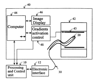
Figure lA provides a block diagram description of the invented apparatus which
includes
a processing and control unit (10), a sensor (20), the module is integrated
into or attached to an
object or a device (30), electronic interface (12), and MRI system (40) with
its main coil (42), three
gradient coils (43), computer (44), gradient coils control unit (48), and
image display (46). The
MRI coils (42 and 43) are presented in more details in Figure 1 B with the
different coils displaced
along the MRI main axis to clarify the presentation.
Figure 2 presents the activation sequence of the MRI gradient coils as
functions of time
during a standard spin echo scan. The steep rise and drop of the generated
magnetic fields result
with high rate of change of the magnetic flux through the coils.
Figure 3A presents the time-derivative of the magnetic fields of the MRI
gradient coils
(which are presented in Figure 2) as functions of time. Figure 3B presents the
voltages induced by
the time-varying magnetic fields of the MRI gradient coils (those presented in
Figure 2 and 3A) in
two orthogonal sensing coils (e.g. 22, 24) as functions of time.
Figure 4A provides a schematic configuration of three orthogonal coils (22,
24, 26) in the
sensor (20) and the induced voltages in each coil. Figure 4B presents an
example of the vectorial
summation of the voltages induced in each coil during activation of the
magnetic field of the Z-
gradient coil into a voltage vector termed Vz.
Figures SA-SD illustrate three potential configurations of coils which provide
a set of three
orthogonal coils or pairs of coils. Figure SA shows a cubic configuration for
extra-corporeal
applications with three orthogonal coils having a typical size of up to 10 mm.
Figure SB shows a
cubic configuration with 3 orthogonal pairs of parallel coils. Figures SC-SD
show a cylindrical
configuration for use with catheters with a typical diameter of 2-3 mm. Figure
SC illustrates an
axial (along the K axis) view, while Figure SD shows a 3-dimensional display
of the sensor, having
one cylindrical coil (22) and two pairs of transverse "saddle" coils (24, 26).
CA 02341662 2001-02-22
WO 00/13586 PCT/US99/20216
Figure 6 presents a block diagram of the measurement and processing system,
including the
sensor (20), the electronic interface (12) and the processing and control unit
(10).
Figure 7 presents a block diagram of the preferred embodiment of the tracking
methodology
for various clinical uses.
Detailed Description of the Preferred Embodiment
Referring now to Figure 1, a typical MRI system (40) has several modules which
are
specifically relevant to the current invention: the three gradient coils (43),
the gradient coils control
unit (48), and the image display (46). The exact implementation of the
invented methodology
depends on the MRI mode of imaging, and the following presentation relates, as
a typical example,
to a standard MRI spin-echo imaging mode. During the spin-echo protocol,
repeated generation of
magnetic fields by the 3 gradient coils provide the spatial encoding of the
received MR echo and
enable the reconstruction of the image. A sample sequence is given in Figure 2
(recorded from a
Signa MRI system, General Electric, USA). For this sequence the system
activates the Z-gradient
coil for "slice selection", simultaneously the X and Y gradient coils for
"phase encoding" and the
X gradient coil for the "read out" phase.
The gradient control unit (48) provides the processing unit (10) with real-
time presentation
of the activation sequence of the three gradient coils which generate the
magnetic gradients (Figure
2). The magnetic fields which are generated by the gradient coils have
components in all three axes
(X,Y,Z), but each of the coils has a precise linear change of the amplitude of
the Z-component
along one axis only, where these coils and the generated magnetic gradients
are termed by this
specific axis (i.e. for the Z-gradient (Gz) the Z-component varies linearly
with the Z-coordinate,
for the X-gradient (Gx) the Z-component varies linearly with the X-coordinate,
and for the Y-
gradient (Gy) the Z-component varies linearly with the Y-coordinate). 'The
other components of
the magnetic fields of the gradient coils have a specific spatial distribution
which depends on the
specific design of the gradient coils. A full description of the magnetic
field as function of time and
location with any mode of operation (G(t,x,y,z)) can be calculated within the
processing unit (10)
by vectorial summation of the three time-variable magnetic fields of the
gradient coils and the time-
CA 02341662 2001-02-22
WO 00/13586 PCT/US99/20216
9
invariant main field (Bo) of the MRI scanner (in the following presentation
vectors are underlined,
to distinguish from scalars):
( 1 ) G(t,x,y,z) = Gx(t,x,y,z) + Gy(t,x,y,z) + Gz(t,x,y,z) + Bo(x,y,z)
where x,y,z are coordinates along the three axes of the MRI coordinate system
(X, Y, Z,
respectively) and t is a time variable. Additional magnetic fields, which are
generated by the RF
(radio frequency) coils of the MRI, are not being used by the current
invention. These fields, which
alternate in the range of mega-hertz, induce high-frequency electrical
potentials in the sensing coils
which can be removed by low-pass filtration.
In one preferred embodiment (Figure 4A), the sensor (20) consists of a set of
three
orthogonal sensing coils (22, 24, 26). The time varying magnetic field
G(t,x,y,z) induces electric
potential, or voltage (V), in each of the sensing coils, and the magnitude of
the induced voltage is
related to the time-derivative of the magnetic flux D through the coil, as
given by Faraday Law:
(2) V = -d~/dt
the magnetic flux at each location is determined by the magnetic field
G(t,x,y,z), the coil
area (A), and the direction of the magnetic field with respect to the spatial
orientation of the coil,
as defined by a unit vector n vertical to the plane of the coil:
(3) O = G(t) ~ n A
where the dot denotes a vectorial dot product.
Combining equations 1 - 3, the induced voltages in the coils are directly
related to the time
derivative of the magnetic field:
(4) V = -d ~ (Gx(t,x,y,z) + Gy(t,x,y,z) + Gz(t,x,y,z) + Bo(x,y,z)~ ~ n A ~ /dt
CA 02341662 2001-02-22
WO 00/13586 PCT/US99/20216
If the sensor does not move or rotate, the Bo field and the direction vector n
are constant and
the induced voltage in each coil is given by:
(5) V = -d ~(Gx(t,x,y,z) + Gy(t,x,y,z) + Gz(t,x,y,z))~ /tit ~ n A
5
The measured magnitudes of the induced voltages at the three coils and the
known magnetic
field G(t,x,y,z) as function of time at each point in the operating field {as
calculated by summing
the individual magnetic fields of all gradient coils which are active at a
specific time) enable the
estimation of the object location and direction by the following sequence of
steps. This sequence
10 of steps is only one option out of several possible approaches which are
similar in concept and only
differ in the actual embodiment of the estimation process.
Step 1. Measurement oJinduced voltages
The induced voltages in the three orthogonal coils (Figure 4) enable the
calculation of the
magnetic fields of the gradient coils at the location of the sensor without
knowing the orientation
of the sensor. While the magnitudes of the induced voltages at each coil
change with the
orientation, their vectorial sum is independent of the orientation and is
proportional to the time-
derivative of the magnetic field at the location of the sensor, as given by
equations 4 and 5. For
example, during activation of the Z-gradient, the time-varying magnetic field
induces three voltages
in the three coils. For a configuration with three orthogonal pairs of
parallel coils (Figure SB), the
induced voltages in two parallel coils of each pair are averaged and the
results are analyzed
similarly as with three single coils.
Thus during activation of the Z-gradient the three voltages Vz~, Vzj, Vzk
correspond either
to the measured voltages in the three single coils or are the averages of the
measured voltages in
each of the three pairs of coils. We define the induced voltages as vectors
Vz~, Vzj, Vzk with
magnitudes equal to the induced voltages in each coil and directions defined
by unit vectors vertical
to the corresponding coil plane (Figure 4A). The vectorial sum of the three
vectors, denoted Vz, is
in the direction of the time-derivative of the local magnetic field of the Z-
gradient:
CA 02341662 2001-02-22
WO 00/13586 PCT/US99/20216
11
(6) Vz =
-[d(Gz(t,x,y,z))/dt~n; A) n; - [d(Gz(t,x,y,z))/dt~n~ A) n~ -
[d(Gz(t,x,y,z))/dt~nk A) nk
This can be easily demonstrated if we break the time derivative of the
magnetic field vector
(dG(t)/dt) into three orthogonal components which are in the directions of
three orthogonal coils.
Since components parallel to the plane of each coil do not induce any voltage,
the induced voltages
Vz~, Vz~, Vzk are proportional to the three components of the time derivative
of the magnetic field
and their sum is in the same direction as the time derivative of the magnetic
field (dG(t)/dt).
Finally, the magnitude of the voltage vector is proportional to the magnitude
of the time-
derivative of the magnetic field of the Z-gradient at the location of the
coils and at the time of
measurement (Figure 4B):
I S (7) ~Vz~ _ ~ (d(Gz(t,x,y,z))/dt) A ~
The magnitudes and directions of the time-derivative of the local magnetic
fields of the X
and Y gradients, or of any combination of two or three magnetic fields of
different gradient coils,
are related (i.e. have the same direction and proportional magnitude) to the
vectorial sum of the
2U induced voltages in the three coils, as described above for the Z-gradient.
The proportionality coefficient of the relation between the magnetic field and
the induced
voltage in a coil is determined by the geometry of the coils, i.e. by A, the
total area of the coil (if
a coil with multiple loops is used the total area is the sum of all areas of
the individual loops).
During a typical sequence of MRI scanning two or even all the three gradient
coils can be
activated at the same time. The magnetic fields of the gradient coils are
known for a specific MRI
scanner by simulation, based on the known geometry of the gradient coils, or
by measurement of
the fields as function of location during activation of each gradient coil.
The activation sequences
of each gradient coil as function of time are provided by the MRI scanner as
analog signals (Figure
CA 02341662 2001-02-22
WO 00/13586 PCT/US99/20216
12
2) or digital data. The known magnetic field and the activation sequence of a
specific gradient coil
can be used to calculate the magnetic field at each spatial location and for a
specific time point, or
to calculate the time derivative of the magnetic field by analog or numerical
differentiation (Figure
3A). This information can also be used to separate magnetic fields which are
generated by
simultaneously activated two or three gradient coils. For example, in Figure 2
the Z-gradient coil
is activated alone, while the X-gradient coil is activated alone or together
with the Y-gradient coil.
The magnitude and orientation of the magnetic field of the X-gradient coil can
be determined from
its independent activation, and this information can be used to eliminate the
contribution of the
magnetic field of the X-gradient coil from the induced voltages measured
during simultaneous
14 activation of the X and Y gradient coils and to extract the magnitude and
orientation of the
magnetic field of the Y-gradient coil.
An alternative, more general approach is to reconstruct the reference magnetic
fields, which
are used in the estimation process (as detailed below), as a superposition of
the simultaneously
1 S activated magnetic fields of different gradients. Thus for each time
point, the activation sequences
of the coils are used to determine the active fields and their magnitude at
that time, and the overall
field is calculated by adding the field contributions from all active coils,
as shown is Equations 4
and S. The location of the device is estimated by comparing the measured
voltages (during
simultaneous activation of more than one gradient) to time derivative of the
reference, composite
20 magnetic field.
Step 2: Transformalion from measured voltages to magnetic fields
The measured voltages are proportional to the time-derivative of the magnetic
fields, and
the proportionality coefficient is determined by the properties of the sensing
coils (i.e. the area of
25 each loop and the number of loops). As explained above, the time-derivative
of the magnetic field
is at the same direction as of the voltage vector (e.g. Vz for Z-gradient) and
its magnitude can be
calculated by re-arranging equation (7):
(8) ~ d(Gz(t,x,y,z))/dt ~ _ ~ Vz ~ / A
CA 02341662 2001-02-22
WO 00/13586 PCT/US99/20216
13
Modern MRI scanners use crushers in association with each activation of a
gradient.
Typically, the crushers are spike-like rapid activation and deactivation of
the gradient coil. For
example, in a General Electric Signa MRI scanner these crushers follow the
shape of a triangle
(Figure 2) or trapezoid, and their time-derivative is similar to a positive
pulse function (the up-slope
S of the crusher) and a negative pulse function (the down-slope of the
crusher) (Figure 3A). The
induced voltages are linearly related to the time derivative of the gradient
field (Equations 4 and
5) and follow the same pattern (Figure 3B). For linear activation and de-
activation of the gradients,
the induced voltages during each constant phase (i.e. up-slope and down-slope)
can be averaged to
yield a value which is directly used to calculate the amplitude of the time-
derivative of the magnetic
field by equation 8. Furthermore, by measuring the time of activation or de-
activation of the
gradients (e.g. 0t), the amplitude of the actual magnetic field can be
calcuiated by (for linear
activation and deactivation patterns):
(9) Gz(t,x,y,z) = d(Gz(t,x,y,z))/dt * Ot
In the following presentation the determination of the location and
orientation is based on
using the magnetic field rather than their respective time-derivative. This is
possible if the slope of
the gradient activation pattern is linear and known, yet a similar procedure
can be implemented by
using the time derivatives of the magnetic fields. The magnetic fields are
provided by a set of 3-
dimensional maps, for example by using Cartesian coordinate system with X,Y,Z
coordinates. For
each location, the magnetic field vector can be mapped as a set of magnitude
and direction
descriptors (e.g. two angles in a spherical coordinate system), or as a set of
three orthogonal
components of the field vector.
Step ~: Estimation of the location xyz of the device in the MRI coordinate
system
By knowing the 3-dimensional distributions of the magnetic fields of the X,Y
and Z
gradients (or a combination of 2 or 3 gradient fields), the instantaneous
location of the device can
be estimated. A search algorithm finds a specific location which, during the
activation of the
gradients, has magnetic fields with similar magnitudes as those calculated
from the measured coil
voltages. A typical search algorithm minimizes a cost function which is based
on the level of
similarity between the estimated fields and the reference known fields at the
assumed location, for
CA 02341662 2001-02-22
WO 00/13586 PCT/US99/20216
14
example a least squares cost function is the sum of the squares of the
differences between each of
the estimated magnetic fields and the corresponding reference fields at the
current estimated
location.
Several problems can hamper the accuracy of the estimation - the search
algorithm may find
a local minima of the cost function (i.e. a wrong solution), the cost function
may be flat or noisy
at the region of the minima which may result in a non-accurate solution, and
the minimized function
may have more than one solution (non-unique solution).
The problem of local minima can be solved by using search algorithms which
guarantee the
convergence to the true, global minima. For example, a grid search evaluates
the cost function ali
over the potential range of solutions. For the current invention, a grid-
search which evaluates the
cost function at all combinations of x,y,z coordinates at a resolution of 1 cm
was found to guarantee
convergence to the global minima.
The accuracy of the estimation critically depends on the signal-to-noise ratio
of the
measurements. When only few measurements are used, for example in our case
three unknown
location variables are calculated from only three measurements (the amplitudes
of the three voltage
vectors), any noise will bias the estimation results. The effect of noise can
be reduced when more
measurements are used and a least-squares estimation algorithm is applied.
This can be achieved
by using more coils, for example a set of six coils, arranged as three
orthogonal parallel pairs with
known distances between the parallel coils. Obviously, more coils will
generate more data with a
high cost of more complex processing apparatus.
The problem of non-uniqueness of the solution is associated with multiple
minima, for
example due to symmetry in the cost function. The typical spatial distribution
of the gradient fields
in commercial MRI systems has symmetry in the three axes, and as a result up
to eight equivalent
minima may exist on the cost function with up to eight different solutions for
the estimation
process. Multiple solutions are a major limitation for any tracking method,
and additional data must
be used to reduce the number of solutions.
CA 02341662 2001-02-22
WO 00/13586 PCT/US99/20216
Step4: Calculation of angles between the voltage vectors
The magnetic fields are vectors, and at each point of the imaging field the
orientations of
the magnetic fields of the three gradients are typically different, and can be
used as additional
information for the estimation process. Since the orientation of the device
relatively to the MRI
5 coordinate system is still unknown at this stage of the estimation process,
the angles between the
three gradient vectors are used instead of the global orientations of the
vectors with respect to the
MRI scanner coordinate system. The angle between any two vectors can be
determined by vector
algebra and analytic geometry. For example, the angle a between the voltage
vector Vz, which is
induced by the Z-gradient, and the voltage vector Vx, which is induced by the
X-gradient, is
10 determined by calculating the squared amplitude of the vectorial difference
between the two
vectors:
(10) ~Vz - VX~2 = (Vz~ - Vx~)2 + (Vz~ - VX~)2 + (Vzk - Vxk)2
15 where Vz;, Vz~, Vzk and Vx~, Vx~, Vxk are the measured voltages in the
i~j,k coils during
activation of the Z-gradient coil and the X-gradient coil, respectively, and
then calculating the angle
between the two vectors by applying the cosine law:
(11 ) COS(a)= ( ~Vz~2 + ~Vx~2 - ~Vz - Vx~2 ~ / (2 * ~Vz~ * Vx~)
where ~Vz~ and (Vx~ are the magnitudes of the voltage vectors induced by the Z
and X
gradients, respectively.
The measured angles are compared to reference angular field maps, which can be
generated
from the 3-dimensional field maps of the three gradients using the same
approach as described by
equations 10 and 11.
In the estimation process, the measured angles are compared to the reference
angles at the
estimated location in addition to the comparison of the magnetic fields
amplitudes. This additional
information improves the accuracy of the estimation process and eliminates the
problem of non-
CA 02341662 2001-02-22
WO 00/13586 PCT/US99/20216
16
uniqueness due to symmetry of the magnetic fields in the XY-plane of the MRl
gradient coils.
Using the amplitudes of the voltage vectors and the angles between the
vectors, there are
still two equivalent anti-symmetric solutions which have the same cost-
function. The gradient fields
of the MRI scanner are anti-symmetric - for example for a set of values of X,Y
and Z coordinates
there exists a point with the opposite X,Y and Z values (i.e. having the same
absolute value but
opposite signs) which has exactly the same absolute magnitudes and angles
between the gradient
field vectors. The distinction between the two anti-symmetric solutions can be
done only during
later stages of the estimation process, as explained below.
Following the grid search, a more accurate location can be found by local
search around one
of the two locations which were found to be the global minima of the cost-
function. Since the two
solutions are anti-symmetric, the local search can be applied around one of
the two solutions and
the final result can be used to find the anti-symmetric solution.
The local search applies a standard search algorithm, for example a Levenberg-
Marquardt
search algorithm, using either the six data points (three amplitudes of the
voltage vectors and three
angles, as detailed above), or with more data when it is available by using
measurements from
configuration with more than 3 coils.
Step S: Determination of the device orientation
Once the spatial location of the sensor in the magnet bore is determined
through steps 1-4,
the X,Y,Z components of the magnetic field at this location during the
operation of any gradient
or gradient combination are known for a specific MRI scanner from the
reference 3-dimensional
magnetic field maps of the gradient coils. Using the voltages measured in each
of the 3 coils during
the activation of the gradients, the three rotation angles which transform
from the MRI reference
coordinate system to the local, device-attached coordinate system, are
determined by an iterative
optimization procedure. Furthermore, at this phase only one of the two anti-
symmetric solutions
provides a minimum of the new cost function, and a unique solution results.
An initial value of the three rotation angles is used to transform the X,Y,Z
components of
CA 02341662 2001-02-22
WO 00/13586 PCT/US99/20216
17
the magnetic fields of the three gradients into the components of the magnetic
fields in the local
(device) coordinate system I,J,K. According to Euler's Rotation Theorem, any
spatial rotation can
be described by three rotation angles, and various conventions exist for these
angles. For example
one convention (which is typically referred to as the Euler angles), is based
on rotation around the
Z axis by angle "c~", followed by rotation around the new X axis by angle "8",
and finally rotation
around the new Y axis by angle "fir". The three rotations can be described by
a rotation matrix:
r" r,z r,3
(12) R = r2, r22 r2s
r3, rs2 r33
where the rotation matrix terms are given by:
r~ i = cos(~r)*cos(~)-cos(6)*sin(~)*sin(~r);
r~2 = cos(~r)*sin(~)+cos(6)*cos(~)*sin(t~r);
rt3 =sin(i~r)*sin(6);
r2a =-sin(>~r)*cos(c~)-cos(6)*sin(~)*cos(>~r);
r22 =-sin(~r)*sin()+cos(8)*cos(c~)*cos(>!r);
r23 =cos(~r)*sin(6);
r3 ~ =sin(8)*sin(~);
r32 =-sin(6)*cos(c~);
r33 =cos(6);
Using the rotation matrix, the magnetic field vector in the reference
coordinate system of
the MRI scanner (i.e. in the X,Y,Z system, with components Gx, Gy, Gz) can be
presented in
another, rotated coordinate system. If a local coordinate system I,J,K is
attached to the device, and
is rotated by the three rotation angles {~,6,i~r} in reference to the X,Y,Z
system, the three Cartesian
components of the magnetic field vector in the rotated system (Gi, Gj, Gk) are
found by:
Gi r» r~2 r~s Gx
(13) Gj - r2~ r22 r2s ~ Gy
Gk r3~ rs2 ras Gz
CA 02341662 2001-02-22
WO 00/13586 PCT/US99/20216
18
The calculated components of the gradient magnetic field in the I,J,K local
system can be
compared with the measured components in order to determine the three unknown
angles of
rotation. These three unknowns can be solved from the three components of one
gradient field, but
the results may be biased due to noise in the measurements. Better results can
be achieved by using
data from more gradients. Since all the three gradient fields are activated
during every MRI
scanning, the preferred embodiment of solving for the three angles of rotation
involves the use of
nine gradient field components, including 3 components for each of the 3
gradients fields (or 18
components if a set of 6 coils is used) and an optimization algorithm, for
example the least squares
method which is described above, to solve for the best solution.
Unlike the situation with absolute values of the measured voltages, which
results with a
non-unique solution composed of the true solution and an anti-symmetric one,
the use of the actual
measurements in each coil during the activation of each gradient or a
combination of two or three
gradients provides a unique solution. The gradient field components in the two
locations, which
correspond to the two solutions, have the same absolute values but opposite
directions, so the
induced voltages in each coil have opposite signs. Although a more rigorous
mathematical analysis
can be used to prove the uniqueness of the solution at this phase of the
estimation process, a
numerical example is provided as a simple demonstration.
For a specific location (e.g. x=20.5 cm, y=10.5 cm, z=l5cm) and three rotation
angles (e.g.
~ _ -40, 8 = 80, >Ir = 0) the induced voltages in the three orthogonal coils
during activation of a X-
gradient, Y-gradient and Z-gradient are given in Table 1 (units are arbitrary
and the simulation is
based on maps of the gradient fields of a Signa MRI scanner). For this
location, the absolute values
of the voltage vectors and the angles between these vectors are calculated and
given in the Table.
Estimation of the location, using only the amplitude of the voltage vectors,
results with eight
potential solutions which all have the same absolute values of the vectors.
The angles between the
voltage vectors are different in 6 of the 8 solutions, leaving only two
equivalent solutions (the input
location and the anti-symmetric solution x= - 20.5 cm, y = -10.5 cm, z = - 1
Scm). Comparison of
the components of the voltage vectors shows that they have opposing signs in
the two locations,
which enables the determination of the true location of the sensor.
CA 02341662 2001-02-22
WO 00/13586 PCT/US99/202t6
19
Step 6: Improving the estimation accuracy by using measurements from all coils
Steps 1-5 described a preferred embodiment of the invention using a two-tier
estimation
process, the first one determines the location and the second one determines
the orientation of the
object or the device, when only three orthogonal coils are used or when the
measurements from the
two coils in each pair are simply averaged. However, when all the measurements
are used in the
estimation process a more accurate estimation result can be achieved.
The estimation process aims to find the 6 unknowns which fully define the
spatial location
and orientation of the sensor. Since the exact distance between the two coils
of each pair is
accurately known, the estimation process still aims to find 6 unknowns, for
example the location
and orientation of a set of three orthogonal coils, while the location and
orientation of the second
set of the three orthogonal coils can be defined with respect to the location
and orientation of the
first set. Thus, although we get more measurements ( 18 voltages for the 6
coils during operation
of each_of the three MRI gradient coils) we still have the same number of
unknowns. A larger
amount of data for the estimation process is a key for more accurate solution
of the optimization
process.
The effect of voltages induced by the Bo field when the sensor moves or
rotates
Equation 4 provides the general description for the induced voltages in the
sensor coils, but
the description above assumes no effect of the Bo field. This assumption is
correct as long as the
sensor does not move, or when the movements are relatively slow. Since the
typical rise time of
gradients in modern MRI system is 1 millisecond (Figure 2), and body or device
movements are
typically slower (in scale of seconds or tenth of a second), the effect of the
Bo can be eliminated
by appropriate high pass filtering of the signals from the sensor coils (for
example a 100 Hz cut-off
frequency), and the description above can be applied on the filtered signals
during movements and
rotations of the body organs (e.g. the head) or the device.
Yet the voltages induced in the sensor coils by the Bo magnetic field can be
advantageously
used to improve the tracking of the location and the orientation of the device
or the object. Unlike
the gradient fields which change in time, the Bo is constant and it induces
electric potential in the
sensor coils only when there is rotation of the coils which change the
magnetic flux through the
CA 02341662 2001-02-22
WO 00/13586 PCT/US99/20216
coils. Unlike equation 3 above, the time varying variable now is the direction
of the coils which is
given- by a time variable unit vector n(t):
(14) O = G ~ n(t) A
5
By applying low-pass filter on the sensor signals the Bo-induced voltages can
be extracted
and used to estimate the time change of the sensor orientation, i.e. the three
angular velocities of
the device or the sensor. This information can be used to improve the
estimation process based on
the magnetic fields of the gradients (e.g. by providing a better initial guess
to the iterative
10 estimation processes) or to enable better prediction of future location and
orientation of the device
or the sensor.
Preferred Embodiment of the Sensor
15 The preferred, minimal configuration of the sensor includes three coils.
The disclosed
invention covers also a lesser configuration of two coils, using the same
approach as presented
above, and using the 6 potentials induced by the three MRI gradients in the
two coils to calculate
the 6 unknowns (3 locations and 3 rotation angles). However, for optimal
performance more data
should be used to reduce the effects of noise and to improve the accuracy of
the tracking. A
20 potential configuration with three orthogonal coils is presented in Figure
SA. This configuration
is suitable for extra-corporeal applications, for example devices for minimal
invasive procedures
like biopsy guns or surgery instruments. Furthermore, the inner space of the
sensor can be used to
contain electronic circuitry, powered by a miniature battery, for signal
conditioning (e.g. filtration
and amplification), signal transformation (e.g. into optical signal, or into
frequency modulated (FM)
signal), or for wireless transmission of the measured potentials.
A more complex configuration is presented in Figure SB, where three pairs of
parallel coils
can be used instead of three single coils, i.e., a total of 6 coils is used in
a sensor. The major
advantage of this configuration is a substantial increase in the accuracy of
the tracking, since for
each activation of any MRI gradient, six, rather than three, different
potentials are induced, and a
total of 18 measurements is available to estimate the 3 unknown location
variables and the 3
CA 02341662 2001-02-22
WO 00/13586 PCT/US99/20216
21
unknown rotation angles with each cycle of scanning. Although the distance
between each of the
two parallel coils is small (e.g. 5-10 mm in the cubic configuration of Figure
SA and 1-2 mm in the
cylindrical configuration of Figure SC and SD), the steep gradients used with
modern MRI scanners
on one hand, and the availability of the exact distance between the two
parallel coils on the other
hand, enable the use of this information to increase the accuracy of the
tracking.
A second preferred configuration is presented in Figure 5 C and D, and
includes a cylindrical
coil and two pairs of "saddle" coils positioned in orthogonal directions to
the cylindrical coils and
to each other (Figure SC presents an axial view of the set of coils and Figure
SD presents an
isometric view of the two pairs of saddle coils and an inner cylindrical
coils, all three coils are
axially displaced to clarify the presentation). This configuration is
specifically useful for catheters
tracking since it has a hollow cylindrical structure and it can be fixed on
the tip of any catheter
without blocking the lumen of the catheter. It can be used with stmt placement
apparatus, with
various diagnostic catheters (e.g. for infra-cardiac electrophysiology
studies) and with current or
1 S future therapeutic catheters (e.g. RF ablation, laser ablation,
percutaneous transmyocardial
revascularization (PMR), targeted drug delivery, local genetic substance
placement, etc.).
In a variant of the cylindrical hollow configuration the two pairs of "saddle"
coils are
replaced by two planar coils, which may be positioned inside or outside the
lumen of the cylindrical
coil. Although this configuration partially blocks the catheter Lumen, it is
simpler to manufacture
and may be useful with applications which do not require free lumen.
The sensors can be assembled from individual coils, for example by glueing 6
small flat
coils on the 6 surfaces of a cube. On a catheter, one pair of coils has a
cylindrical shape and can be
directly wired over the shaft of the catheter, while the two other pairs have
saddle shape, and can
be glued around the cylindrical coils. Another potential approach for the
construction of the multi-
coil sensor is by using flexible printed electrical circuits, which include
all the coils and are folded
to achieve the 3-dimensional shape.
CA 02341662 2001-02-22
WO 00/13586 PCT/US99/20216
22
Preferred Embodiment of the Tracking Apparatus
The tracking apparatus (Figure 6) includes the sensor 20, the electronic
interface 12, the
processing module 10, and the interface with the MRI scanner. It can be custom-
designed and built
for the specific tracking application or assembled from commercially available
components.
S
The electronic interface (12) contains a set of amplifiers (122) to amplify
the low-voltage
potentials which are induced in the coils (from millivolts level to volts), a
set of low-pass filters
(124) to eliminate the high frequency voltages which are induced by the RF
transmission, having
frequency range of 10-400 MHz (depending on the MRI magnet strength), and stop-
band or notch
filter (126) to remove potentials induced by the step-wise increase of the MRI
gradients, which in
a General Electric MRI scanner produce a 128KHz artifact. Various commercial
systems with
programable amplifier~filter combinations can be used to amplify and filter
the low-voltage signals
from the sensors (e.g. SCS-802, Alligator Technologies, Costa-Mesa, CA).
The processing and control unit (10) can be developed using readily available
commercial
hardware. For example, the measured signals from the sensor can be digitized
by analog-to-digital
(A/D) converter (102) using a standard data acquisition board (e.g. National
Instruments, Austin,
TX), and processed in real-time by a modern, high performance processor 104
(e.g. a Pentium III
processor with MMX built-in DSP). Another potential solution, which provides
faster estimation
rates, can be based on digital signal processor (DSP) boards, having built-in
or attached A/D
converter having at least 6 channels (3 coil signals and 3 MRI gradient
signals), high-performance
DSP for iterative solution of location and orientation, su~cient memory
capacity for the program
and for data (e.g. the reference magnetic fields), and communication bus for
interface with the host
computer or directly with the MRI scanner (e.g. Blacktip-CPCI processing board
and BITSI-DAQ
analog input/output adapter, Bittware Research Systems, Concord, NH). The
software for the DSP
or the PC processor can be developed with standard programming languages, for
example C++ or
assembly. We have used the Matlab software development environment (The Math
Works, Natick,
MA) to rapidly implement the estimation process as described above.
The interface with the MRl includes two main components - a channel to
transfer the real-
time location and orientation of the sensor, and a channel (or channels) to
transfer the activation
CA 02341662 2001-02-22
WO 00/13586 PCT/US99/20216
23
pattern of the gradient coils from the MRI scanner to the processing module.
Either digital
communication channel, analog channels, or a combination of the two can be
used. With the Signa
MRI system, for example, the gradient activation sequence is available as
standard analog output
from the gradient control system, and tracking information can be received by
the MRI through a
standard serial communication line.
The overall operation of the tracking system is presented below and in Figure
7. The
induced potentials in the sensors (700), typically having a magnitude of
millivolts, are amplified
and filtered by the electronic interface module (710). The activation pattern
from the MRI scanner
(702) is transferred to the tracking system through the MRI interface module
(704) and may be
processed by the electronic interface module (e.g. filtered) before it is
digitized by the processing
module. The activation pattern of the MRI gradients (Figure 2) is analyzed by
the processor to
determine the activation of each of the gradient coils, e.g. by threshold
triggering (712). Typically
we will use the crushers which have longer activation times and higher
amplitude of magnetic
1 S fields. Once an activation of any gradient coil is detected, the processor
digitizes the signal from
the coils and process it to determine the level of the induced signals {714).
If the activation of the
gradient is linear, its time-derivative during the activation is flat (Figure
3A) and the induced
potential in the sensor coils is also flat {Figure 3B). Thus, the measured
signals can be averaged as
long as the gradient activation is on. It should be noted, however, that non-
linear activation patterns
can be used as long as a description of the activation pattern of the gradient
coils is available. The
measured signals from the three orthogonal coils are calibrated into magnetic
fields units using the
calibration factors of the coils (Equations 8 and 9). The measured induced
voltages in the set of
orthogonal coils are used to calculate the amplitude of the voltage-vector
(Equations 6-7) and the
angles between the voltage-vectors of the different MRI gradients (Equations
10-11 ) (716). These
amplitudes and angles are used to estimate the location of the sensor in the
MRI coordinate system
(block 718, 3) and to estimate the orientation of the sensor (block 720, 4).
The estimated location
and orientation may be further processed to improve the quality of the
tracking, e.g. by the
application of a low-pass digital filter on the estimations at a specific
time, using previous
estimations, and may be transformed into a data format which is required by
the MRI scanner (722).
Finally, the tracking data (724) is transferred to the MRI scanner through the
MRI interface module
(704).
CA 02341662 2001-02-22
WO 00/13586 PCT/US99/20216
24
Clinical Applications
The determined location and orientation of the sensor can be transferred to
the MRI scanner
in real-time and used for various tasks, for example for real-time control of
the scanning plane, to
display the location and orientation of the object or the device with the
tracking sensor on the MR
image, to correct motion artifacts. Potential clinical applications ofthe
invention can be divided into
applications for diagnostic MR imaging and for interventional MRI.
Dia;~nostic MRI: A major problem with MR imaging is motion artifacts due to
patient movement.
With high-resolution scanning, which may require image acquisition during many
seconds and even
minutes, patient movement and breathing may induce motion artifacts and
blurred images. MR
scanning is specifically sensitive to movements during phase contrast
angiography, diffusion
imaging, and functional MRI with echo-planar imaging (EP)]. Using the present
invention for real-
time determination of the location and orientation of the scanned object can
reduce the effect of
motion on the MR scans by real-time control and correction of the scanning
plane, in order to
compensate for the movement, or by post-acquisition image processing.
Interventional MRI: The sensor can be used with various devices, like
miniature tools for minimally
invasive surgery, catheters inside blood vessels, rigid and flexible
endoscopes, biopsy and aspiration
needles. It can be used to measure the location of the device with respect to
the MRI coordinate
system and to enable the MR scanner to present the device location on the MR
images, as visual
feedback to the operator, or to calculate and display the line of current
orientation to assist the
operator to steer the device into a specific target. Another potential
application is to slave the MRI
plane of imaging to the tracking sensor, for example to apply high resolution
imaging on a small
volume around the site of a catheter, for better imaging of the region of
interest to improve
diagnostic performance or to control the effect of an intervention (e.g radio-
frequency, cryo, or
chemical ablation and laser photocoagulation can be monitored by temperature-
sensitive MR
imaging). Another potential application is to use the information of the
location and orientation of
the device in order to enable display of the MRI images in reference to the
device local coordinate
system, as if the operator is looking through the device and in the direction
of the tip, similar to the
use of optical endoscopes. One more application is to use the location
tracking in order to mark
location of previous interventions on the MRI image.
CA 02341662 2001-02-22
WO 00/13586 PCT/US99/20216
An application with great clinical importance, where using MRI guidance is of
specific
advantage, is percutaneous myocardial revascularization (PMR). PMR is
typically performed during
cardiac catheterization. A laser transmitting catheter is inserted through the
femoral artery up
through the aorta into the left ventricle of the heart. Based on prior
perfusion studies (e.g. Thallium
5 scan) or indirect information on viability of the myocardium (e.g. by
measurement of local wall
motion), the cardiologist applies laser energy to drill miniature channels in
the inner portion of the
heart muscle, which stimulates angiogenesis and new blood vessel growth. PMR
potentially
provides a less invasive solution (compared to bypass surgery) for ischemic
heart disease patients
which cannot be adequately managed by angioplasty or stmt placement. It may
also be used in
10 conjunction with angioplasty or stems to treat areas of the heart not
completely revascularized by
a balloon or stent placement. Currently, PMR is exclusively done with X-ray
guidance. The main
advantage of MRI is the excellent performance of MRI in the assessment of
myocardial blood
perfusion, through the use of contrast agents. Thus rather than using indirect
information on the
location of poorly perfused regions, a diagnostic session of myocardial
perfusion in the MRI
15 scanner can be followed by immediate intervention, using the existing
perfusion images and real-
time tracking of the laser catheter with the disclosed tracking methodology.
Additional advantage,
unique to MRI, is the potential to control the intervention by high-
resolution, real-time imaging of
the myocardium during the application of the laser treatment. Furthermore,
since PMR is typically
performed on multiple locations, and a good coverage of the treated myocardium
should be
20 achieved, marking the location of the treated locations on the perfusion
image, using the location
data of the tracking system, may provide optimal coverage of the diseased
region.
Anatomically, the tracking sensor can be used for various diagnostic and
interventional
procedures inside the brain (internally through blood vessels or through burr
holes in the scull), the
25 cardiovascular system (heart chambers, coronary arteries, blood vessels),
the gastro-intestinal tract
(stomach, duodenum, biliary tract, gall bladder, intestine, colon) and the
liver, the urinary system
(bladder, ureters, kidneys), the pulmonary system (the bronchial tree or blood
vessels), the skeletal
system (joints), the reproductive tract, and others.
CA 02341662 2001-02-22
WO 00/13586 PCT/US99/20216
26
TABLE 1
Induced voltages in 3 orthogonal coils were simulated for a sample location
(X=20.5 cm, Y=10.5 cm,
Z=15.0 cm) inside an MRI scanner during the activation of three gradients and
are presented in the lower
section of the table as voltage vectors (Vx, Vy, Vz). Using only the absolute
amplitudes of the voltage
vectors (iVx~, ~Vy~, ~Vz~) results with eight different solutions (Xest, Yest,
Zest). The use of the angles
between the voltage vectors (XZ~ang, YZ ang, YX ang) eliminates 6 of the
solutions and provides two
anti-symmetric equivalent solutions ( 1 and 8). Finally, when the three
components of each of the three
voltage vectors are used (Vx, Vy, Vz), a unique correct solution (solution 8)
is obtained.
SolutionSolutionSolutionSolutionSolutionSolutionSolutionSolution
I 2 3 4 S 6 7 8
Xest -20.50 20.50 -20.50 20.50 -20.50 20.50 -20.50 20.50
Yest -10.50 -10.50 10.50 10,50 -10.50 -10.50 10,50 10.50
-15.00 -15.00 -15.00 -15.00 15.00 15.00 15.00 15.00
1 V 27.791827.791827.791827.791827.791827.791827.791827.7918
S
V 19.651319.651319.651319.651319.651319.651319.651319.6513
Vz 19.837019.837019.837019.837019.837019.837019.837019.8370
XZ 9.7436 -7.69287.6928 -9.7436-9.74367.6928 -7.69289.7436
an
YZ -11.1176-5.32375.3237 11.117611.11765.3237 -5.3237-11.1176
an
YX -13.09!)426.750826.7508-13.0904-13.090426.750826.7508-13.0904
an
Vx -16.2143-16.2143-16,2143-16.214316.214316.214316.214316.2143
-21.210317.2907-21.210317.2907-17.290721.2103-17.290721.2103
7.7202 14.50907.7202 14.5090-14.5090-7.7202-14.5090-7.7202
V -12.2805-12.2805-12.2805-12.280512.280512.280512.280512.2805
11.628411.6284-7.5044-7.50447.5044 7.5044 -11.6284-1L6284
-10.0072-10.0072-(3.3808-13.380813.380813.380810.007210.0072
Vz 4.93$3 -12.077112.0771-4.93834.9383 -12.077112.0771-4.9383
-13.2568-15.7361-14.7342-17.213517.213514.734215.736113.2568
-13.90600.1548 -5.52758.5332 -8.53325.5275 -0.154813.9060