Note: Descriptions are shown in the official language in which they were submitted.
CA 02594339 2013-04-19
,
- I -
METHOD AND APPARATUS FOR ESTIMATING FORMATION SLOWNESS
[0001]
Background of the Invention
[0002] This invention relates generally to acoustic well
logging, and in
particular to estimating formation slowness using an acoustic well logging
tool.
[0003] Formation compressional and shear slowness are two of
the most
important parameters used in the exploration and production of hydrocarbon.
Conventionally, they are measured by sonic logging. A sonic logging tool
consists of two primary parts: data acquisition and data processing. Data
acquisition is done by sending a logging tool down into an exploration or
production well, and the acoustic source on the logging tool sends an acoustic
signal that subsequently propagates along the well and is recorded at several
evenly spaced receivers that are some distance away from the source.
Formation compressional and shear slowness are then estimated by
processing the recorded waveforms, using array sonic processing techniques,
such as the slowness-time coherence method (STC).
[0004] Recent studies have shown that STC yields an accurate
slowness estimation when, and only when, the acoustic waves propagated
along a wellbore are non-dispersive, or multiple arrivals contained in the
waveforms are well separated in the slowness-time domain. When the
underlying waveforms are dispersive or the waveforms compose of mixed
modes with similar group velocities, such as in the case of wireline leaky P-
mode (for compressional slowness in very slow formation), wireline dipole
mode (for shear slowness), quadrupole mode (for shear slowness) in logging
while drilling (LWD) or some monopole mode (for compressional slowness) in
LWD, STC produces a systematic error in the slowness estimation. The
amount of those systematic errors is large enough to result in negative
CA 02594339 2007-07-05
WO 2006/078416 PCT/US2005/046827
- 2 -
implications in the exploration and production of hydrocarbons, such as oil
can be mistaken as water in prospect assessment. Furthermore, the
correlogram produced by STC method, currently used as a quality control tool
for slowness estimation by industry, does not reflect the accuracy of the
slowness estimation.
[0005]
Recently, several approaches have been developed to address
the limitations of the existing methods and apparatus for estimating formation
slowness. Theses fall into two categories: model-driven dispersion correction
and phase velocity processing. The model-driven dispersion correction
approaches have been adapted by major logging companies, such as
Schlumberger and Baker Hughes. They have been developed to address
wireline dipole mode and leaky P mode. Baker Hughes also applies its
approach to their quadrupole LWD data. The model-driven approach still
makes use of STC and corrects dispersion effects by applying a theoretically
calculated dispersion curve of the corresponding mode. The
dispersion
correction of the model-driven approach is only accurate under several
assumptions that are hard to meet in reality, including circular borehole,
homogeneous and isotropic formation and good knowledge of a variety of
formation and mud properties, including slowness and density. In the case
where the waveforms contain multiple arrivals that are not well separated in
slowness-time domain, all model-driven methods will not arrive at the correct
formation slowness. The phase velocity processing approach estimate
instantaneous phase slowness for each receiver pairs, which could potential
yield more accurate slowness estimation than STC method. However as the
formation slowness value is computed by averaging over the desired travel
time interval, the phase velocity processing still generates a systematic
error
in slowness estimation. Also the phase velocity processing may suffer some
stability problems.
[0006] The
present invention is directed to overcoming one or more of
the limitations of the existing methods and apparatus for estimating formation
slowness.
CA 02594339 2007-07-05
WO 2006/078416 PCT/US2005/046827
- 3 -
Summary of the Invention
[0007] According to one aspect of the present invention, a method for
estimating formation slowness using waveforms recorded by an acoustic
logging tool is provided that includes extracting a phase slowness coherence
of the recorded waveforms at a plurality of frequencies within a range of
frequencies and phase slownesses; converting the extracted phase slowness
coherence into a formation slowness curve whose magnitude is a function of
the extracted phase slowness coherence; and determining one or more
anomalies within the formation slowness curve; wherein the location of one of
the anomalies of the formation slowness curve is representative of the
estimated formation slowness.
[0008] According to another aspect of the present invention, a method
for determining a quality of a determination of an estimate of a formation
slowness using waveforms recorded by an acoustic logging tool positioned
within a wellbore that traverses a subterranean formation, is provided that
includes extracting a phase slowness coherence of the recorded waveforms
at a plurality of frequencies within a range of frequencies and phase
slownesses; converting the extracted phase slowness coherence into a
formation slowness curve whose magnitude is a function of the extracted
phase slowness coherence; determining one or more anomalies within the
formation slowness curve, wherein the location of one of the anomalies of the
formation slowness curve is representative of the estimated formation
slowness; positioning the logging tool at a plurality of depths within the
borehole; repeating extracting, converting, and determining at each depth;
generating a mapping of the formation slowness curve over a range of the
depths; and generating values for the estimated formation slowness at the
range of depths and constructing a formation estimate curve; wherein the
quality of the estimated formation slownesses determined is a function of a
degree to which the formation estimate curve overlays an edge of the
mapping of the formation slowness curve.
CA 02594339 2007-07-05
WO 2006/078416 PCT/US2005/046827
- 4 -
[0009] According to another aspect of the present invention, a system
for estimating formation slowness using waveforms recorded by an acoustic
logging tool has been provided that includes means for extracting a phase
slowness coherence of the recorded waveforms at a plurality of frequencies
within a range of frequencies and phase slownesses; means for converting
the extracted phase slowness coherence into a formation slowness curve
whose magnitude is a function of the extracted phase slowness coherence;
and means for determining one or more anomalies within the formation
slowness curve; wherein the location of one of the anomalies of the formation
slowness curve is representative of the estimated formation slowness.
[0010] According to another aspect of the present invention, a system
for determining a quality of a determination of an estimate of a formation
slowness using waveforms recorded by an acoustic logging tool positioned
within a wellbore that traverses a subterranean formation has been provided
that includes means for extracting a phase slowness coherence of the
recorded waveforms at a plurality of frequencies within a range of frequencies
and phase slownesses; means for converting the extracted phase slowness
coherence into a formation slowness curve whose magnitude is a function of
the extracted phase slowness coherence; means for determining one or more
anomalies within the formation slowness curve, wherein the location of one of
the anomalies of the formation slowness curve is representative of the
estimated formation slowness; positioning the logging tool at a plurality of
depths within the borehole; repeating extracting, converting, and determining
at each depth; generating a mapping of the formation slowness curve over a
range of the depths; and means for generating values for the estimated
formation slowness at the range of depths and constructing a formation
estimate curve; wherein the quality of the estimated formation slownesses
determined is a function of a degree to which the formation estimate curve
overlays an edge of the mapping of the formation slowness curve.
Brief Description of the Drawings
[0011] Fig. 1 is a schematic illustration of an exemplary embodiment
of
CA 02594339 2007-07-05
WO 2006/078416 PCT/US2005/046827
- 5 -
a system for estimating formation slowness.
[0012] Fig. 2 is a fragmentary cross sectional illustration of the
system
of Fig. 1 during the operation of the system.
[0013] Fig. 3 is a graphical illustration of typical waveforms
detected
during the operation of the system of Fig. I.
[0014] Fig. 4 is a flow chart illustration of an exemplary embodiment
of
a method for operating the system of Fig. I.
[0015] Fig. 5 is a graphical illustration of an exemplary embodiment
of a
phase slowness coherence generated during the implementation of the
method of FIG. 4 by the system of Fig. 1.
[0016] Fig. 6 is a graphical illustration of an exemplary embodiment
of a
curve containing information representative of the formation slowness
generated during the implementation of the method of Fig. 4 by the system of
Fig. 1.
[0017] Fig. 7 is a graphical illustration of an exemplary embodiment
of a
histogram containing information representative of the formation slowness
generated during the implementation of the method of Fig. 4 by the system of
Fig. I.
[0018] Fig. 8A is a flow chart illustration of an exemplary embodiment
of a method for operating the system of Fig. 1.
[0019] Fig. 8B is a graphical illustration of an exemplary embodiment
of
typical waveforms detected during the operation of the method of Fig. 8A.
[0020] Fig. 8C is a graphical illustration of an exemplary embodiment
of
a coherence semblance map extracted during the operation of the method of
Fig. 8A.
[0021] Fig. 8D is an exemplary embodiment of a formation slowness
curve extracted during the operation of the method of Fig. 8A.
[0022] Fig. 9A is a flow chart illustration of an exemplary embodiment
of a method for operating the system of Fig. I.
CA 02594339 2007-07-05
WO 2006/078416 PCT/US2005/046827
- 6 -
[0023] Fig. 9B is a graphical illustration of an exemplary embodiment
of
typical waveforms detected during the operation of the method of Fig. 9A.
[0024] Fig. 9C is a graphical illustration of an exemplary embodiment
of
a coherence semblance map extracted during the operation of the method of
Fig. 9A.
[0025] Fig. 9D is an exemplary embodiment of a dispersion curve
extracted during the operation of the method of Fig. 9A.
[0026] Fig. 9E is an exemplary embodiment of a histogram extracted
during the operation of the method of Fig. 9A.
[0027] Fig. 10A is a flow chart illustration of an exemplary
embodiment
of a method for operating the system of Fig. 1.
[0028] Fig. 10B is a graphical illustration of an exemplary embodiment
of typical waveforms detected during the operation of the method of Fig. 10A.
[0029] Fig. 10C is a graphical illustration of an exemplary embodiment
of a coherence semblance map extracted during the operation of the method
of Fig. 10A.
[0030] Fig. 10D is an exemplary embodiment of a dispersion curve
extracted during the operation of the method of Fig. 10A.
[0031] Fig. 10E is an exemplary embodiment of a probability density
function extracted during the operation of the method of Fig. 10A.
[0032] Fig. 11A is a flow chart illustration of an exemplary
embodiment
of a method for operating the system of Fig. 1.
[0033] Fig. 11B is a graphical illustration of an exemplary embodiment
of typical waveforms detected during the operation of the method of Fig. 11A.
[0034] Fig. 11C is a graphical illustration of an exemplary embodiment
of a coherence semblance map extracted during the operation of the method
of Fig. 11A.
[0035] Fig. 11D is an exemplary embodiment of a formation slowness
CA 02594339 2007-07-05
WO 2006/078416 PCT/US2005/046827
- 7 -
curve extracted during the operation of the method of Fig. 11A.
[0036] Figs. 12A, 12B, 12Cand 12D are flow chart illustrations of an
exemplary embodiment of a method for operating the system of Fig. 1.
[0037] Fig. 121 is a graphical illustration of an exemplary embodiment
of
typical waveforms detected during the operation of the method of Figs. 12A-D.
[0038] Fig. 12J is a graphical illustration of an exemplary embodiment
of a coherence semblance map extracted during the operation of the method
of Figs. 12A-D.
[0039] Fig. 12K is an exemplary embodiment of a formation slowness
curve extracted during the operation of the method of Figs. 12A-D.
[0040] Fig. 12L is an exemplary embodiment of a dispersion curve
extracted during the operation of the method of Figs. 12A-D.
[0041] Fig. 12M is an exemplary embodiment of a histogram extracted
during the operation of the method of Figs. 12A-D.
[0042] Fig. 12N is an exemplary embodiment of a histogram mapping
extracted during the operation of the method of Figs. 12A-D.
[0043] Fig. 120 is an exemplary embodiment of a piece-wise
continuous histogram mapping extracted during the operation of the method
of Figs. 12A-D.
[0044] Fig. 12P is an exemplary embodiment of a piece-wise
continuous histogram mapping extracted during the operation of the method
of Figs. 12A-D.
[0045] Fig. 13A is a flow chart illustration of an exemplary
embodiment
of a quality control method for operating the system of Fig. 1.
[0046] Fig. 13B is a graphical illustration of an exemplary embodiment
of the plotting of a formation slowness estimate curve onto a formation
slowness mapping of the method of Fig. 13A.
[0047] Fig. 14A is a flow chart illustration of an exemplary
embodiment
CA 02594339 2007-07-05
WO 2006/078416 PCT/US2005/046827
- 8 -
of a quality control method for operating the system of Fig. 1.
[0048] Fig. 14B is a graphical illustration of an exemplary embodiment
of the plotting of a formation slowness estimate curve onto a slowness
histogram mapping in of the method of Fig. 14A.
Detailed Description of the Illustrative Embodiments
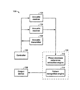
[0049] Referring initially to Fig. 1, a system 100 for estimating
formation
slowness includes a conventional acoustic transmitter 102 and a plurality of
conventional acoustic receivers 104. The acoustic transmitter 102 and the
acoustic receivers 104 are operably coupled to a conventional controller 106.
The acoustic receivers 104 are also operably coupled to a signal processing
engine 110 that includes a phase slowness coherence extraction engine 112
and a pattern recognition engine 114. A conventional output device 116 is
coupled to the signal processing engine 110 and the controller 106. The
design and general operation of the acoustic transmitter 102, acoustic
receivers 104, controller 106, and output device 116 are considered well
known to persons having ordinary skill in the art.
[0050] During operation of the system 100, as illustrated in Fig. 2,
the
acoustic transmitter 102 and the acoustic receivers 104 may be positioned
within a logging sonde 200 and supported within a wellbore 202 that traverses
a subterranean formation 204. In an exemplary embodiment, the acoustic
transmitter 102 and the acoustic receivers 104 are centrally positioned within
the wellbore 202, and the wellbore 202 may, or may not, include a cased
section. The acoustic transmitter 102 may then be operated in a conventional
manner to generate and transmit acoustic signals into and through the
formation 204 that may then be detected and processed by the acoustic
receivers 104 to thereby generate a series of waveforms 300 as illustrated in
Fig. 3.
[0051] In an exemplary embodiment, as illustrated in Fig. 4, during
operation of the system 100, the system implements a method 400 of
estimating formation slowness for the formation in which the waveforms 300
CA 02594339 2007-07-05
WO 2006/078416 PCT/US2005/046827
- 9 -
are processed by the phase slowness coherence extraction engine 112 to
generate the phase slowness coherence 500 at each frequency over
predetermined frequency and slowness intervals in step 402 as illustrated in
Fig. 5. In an exemplary embodiment, as illustrated in Fig. 5, the phase
slowness coherence 500 includes a coherence semblance map 500a and a
dispersion curve 500b, both of which are generated from the waveforms 300.
[0052] In an exemplary embodiment, in step 402, the frequency and
slowness intervals are selected to cover the desired borehole mode, such as,
for example, leaky P, dipole, quadrupole, S or P mode. In an exemplary
embodiment, in step 402, the phase slowness coherence extraction may be
provided as disclosed in one or more of the following: 1) Lang et al.,
Estimating Slowness Dispersion From Arrays of Sonic Logging Waveforms,
Geophysics, Vol. 52, No. 4 (April 1987), p. 530 ¨ 544; 2) U.S. Patent No.
6,691,036; and/or 3) Nolte et al., 1997, Dispersion analysis of split flexural
waves, Borehole Acoustics and Logging/Reservoir Delineation Consortia
Annual Report, MIT.
[0053] In an exemplary embodiment, in step 404, the phase slowness
coherence at each frequency over a predetermined frequency interval
determined in step 402 is then processed by the pattern recognition engine
114 to generate the estimate of the value of the formation slowness. In an
exemplary embodiment, in step 404, the phase slowness coherence
generated in step 402 is converted into a formation slowness curve 600 with
the magnitude of the formation slowness curve being a function of slowness
as illustrated in Fig. 6. Furthermore, in an exemplary embodiment, the
formation slowness is associated with an anomaly of the formation slowness
curve 600. In an exemplary embodiment, the anomaly associated with the
formation slowness value is a local maximum or minimum of the formation
slowness curve 600, and the slowness value for the local minimum or
maximum is representative of the formation slowness. In an exemplary
embodiment, the formation slowness may then be obtained, for example, by
using a conventional optimization method to determine the local maximum or
CA 02594339 2007-07-05
WO 2006/078416 PCT/US2005/046827
- 10 -
minimum of the curve 600.
[0054] In an exemplary embodiment, in step 404, as illustrated in Fig.
6, the magnitude of the formation slowness curve 600 is a function of the 2nd
order derivative of a different formation slowness curve 602 whose magnitude
is a function of a summation across frequencies of the phase slowness
coherence 500.
[0055] In an exemplary embodiment, in step 404, the magnitude of the
curve 600 may be: 1) a summation across frequencies of the nth power of the
phase slowness coherence 500; 2) a summation across frequencies of the nth
order derivatives of the phase slowness coherence; 3) nth order derivatives of
a summation across frequencies of the nth power of the phase slowness
coherence; 4) the probability density function of the phase slowness
population in the dispersion curve 500b; 5) a summation across frequencies
of the nth power of the coherence semblance map 500a; 6) nth order
derivatives of a summation across frequencies of the nth power of the
coherence semblance map; and/or 7) a histogram 700 of the phase slowness
population in the dispersion curve 500b as illustrated in Fig. 7. A threshold
may be used to zero-out small semblance points in advance. Depending on
the data quality and characteristics, the person skilled in the art will be
able to
identify other choices for a formation slowness curve that are suitable for
the
present invention, such as a histogram or probability density function of the
dispersion curve modified by the characteristics of the data. Examples of the
characteristics of the data include but are not limited to wave spectra, the
values of the coherence semblance map at each respective slowness-
frequency point, or the nth power of the the values of the coherence
semblance map at each respective slowness-frequency point. For instance,
suppose at a given frequency, values of the slowness-frequency points on the
coherence semblance map are denoted as P =[Pi P2 = = = Pn] and each
component of p, p, (i=1,2,...n), is associated to a slowness value. The
slowness value, DT, associated with the maximum component of p (denoted
as põõ is taken as the slowness of the wave at the frequency. When
CA 02594339 2007-07-05
WO 2006/078416 PC T/US2005/046827
- 11 -
computing the histogram, the number of slowness values at that frequency is
counted as (n an )1 instead of 1, where an is an integer number closest to pm.
(In the preceding, I and n are real numbers greater than zero.) It should be
understood that the term used herein, "formation slowness curve", can also be
called an "objective function", a term that will be familiar to those who work
in
the field. The objective function must be some quantity that is a function of
slowness, i.e., the formation slowness curve must be such a quantity plotted
vs. slowness. The present invention and the appended claims are not limited
to the specific examples given herein for the formation slowness curve.
[0056] In an exemplary experimental implementation of the method
400, as illustrated in Fig. 5, the phase slowness coherence 500 provided a
frequency domain coherence semblance map and, as illustrated in Fig. 6, the
magnitude of the formation slowness curve 600 was equal to the 2nd
derivative of the summation across frequencies of the coherence semblance
map 500a. A local maximum 604 of the formation slowness curve 600 yielded
a corresponding formation slowness of 215 ps/ft.
[0057] In an exemplary embodiment, the method 400 can be
implemented by the system 100 to generate an acoustic log by repeating the
method at each logging depth. The curve 600, generated from phase
slowness coherence 500, may then be plotted as a color-coded map in the
depth and slowness domains.
[0058] In an exemplary embodiment, the acoustic transmitter 102 and
the acoustic receivers 104 are provided as part of a conventional acoustic
downhole logging tool in which the frequency band and signal-to-noise ratio of
the waveforms 300 are selected to be appropriate for the operating
environment of the selected borehole 202 and formation 204 in a conventional
manner.
[0059] In an exemplary embodiment, during operation of the system
100, several representative samples of waveforms 300 are generated and
analyzed to determine an optimal set of parameters for further operation of
the system 100, when implementing the method 400, such as, for example,
CA 02594339 2007-07-05
WO 2006/078416 PCT/US2005/046827
- 12 -
the frequency and slowness range.
Furthermore, in an exemplary
embodiment, during operation of the system 100, the most suitable quantity
and anomaly that can single out the formation slowness from the curve 600 is
also characterized from any number of sample runs of the system.
[0060] In an
exemplary embodiment, in step 404, the preferred quantity
and anomaly in the curve 600 varies as a function of the characteristics of a
mode and waveform data. In particular, to estimate formation shear slowness
from wireline dipole mode or LWD quadrupole mode, or estimate formation
compressional slowness from wireline leaky P mode, the preferred quantity in
the curve is the summation across all frequencies of the nth power of the
coherence semblance map 500a generated in step 402. The formation
slowness value may then be determined by searching for one of the local
maxima of the first order derivative of the quantity with respect to slowness.
[0061]
Alternatively, if the wireline dipole data or leaky P data contains
significant energy around the cutoff frequency, it is more desirable to
obtain,
in step 404, the histogram, the modified histogram, the probability density
function, or the modified probability density function of the phase slowness
distribution of the dispersion curve 500b generated in step 402, and then
select the formation slowness at a local maximum of the probability density
function or of the histogram.
[0062]
Alternatively, in the case of monopole logging while drilling
(LWD), where the energy of the formation compressional arrival can only
surpass drilling collar arrivals in a frequency stop band, the preferred
methodology for step 404 depends upon the slowness difference between the
drilling collar arrival and formation compressional arrival. When the slowness
of formation compressional arrival differs from drilling collar arrival such
that
the summation of the nth power of the coherence semblance map 500a has
two local maxima, with one of them corresponding to the formation
compressional arrival, the preferred quantity in step 404 can be either the
summation of the nth power of the coherence semblance map 500a or the
probability density function or histogram. The anomaly that is then used to
CA 02594339 2007-07-05
WO 2006/078416 PCT/US2005/046827
- 13 -
determine formation compressional slowness is the local maximum of the
quantity. When otherwise the slowness of formation compressional arrival
and drilling collar arrival is similar, the preferred quantity in step 404 is
the first
order derivative of the summation of the nth power of the coherence
semblance map 500a. The anomaly that is then used to determine formation
compressional slowness is the local maximum/minimum of the quantity.
When the formation compressional arrival is slower than the drilling collar
arrival, the anomaly is a local minimum, otherwise it is a local maximum.
[0063] In several exemplary experimental implementations of the
method 400 using the system 100, the waveforms 300, the phase slowness
coherence 500, and/or the curve 600 were further processed using
conventional data smoothing methods.
[0064] In an exemplary embodiment, operation of the system 100 using
the method 400 provides a method for estimating formation compressional
and shear slowness by a combination of frequency-domain-semblance (FDS)
analysis and automatic pattern recognition (APR) on the waveforms 300. In
an exemplary embodiment, the method 400 is: 1) data-driven; 2) is not
affected by mode dispersion, borehole shape, formation
heterogeneity/anisotropy, and/or 3) is not affected by other formation and mud
properties. In an exemplary embodiment, the method 400 extracts the
formation slowness from dispersive waveforms or waveforms containing
multiple modes that cannot be well separated in the slowness-time domain.
Furthermore, in an exemplary embodiment, the method 400 is able to provide
a correct formation slowness value when a method using slowness time
coherence (STC) produces a correct formation slowness. In an exemplary
embodiment, the method 400 does not average slowness across frequency or
time interval as would be done in a SIC method or phase velocity processing
based methods. In an exemplary embodiment, the method 400 provides a
better quality control map than the conventionally used SIC-based
correlagram, which does not reveal the accuracy of the slowness estimation if
the waveforms 300 are dispersive or if the waveforms are composed of mixed
CA 02594339 2007-09-19
- 14 -
modes that are not well separated in the slowness-time domain.
[0065] Referring to Fig. 8A, in an exemplary embodiment, the system
100 implements a method 800 for estimating a value for the formation
slowness in which, in step 802, waveform data wi(t), for I = 1 to N, where N =
number of acoustic receivers 104, as illustrated in Fig. 8B, are extracted by
operating the acoustic transmitter 102 and acoustic receivers 104 in a
conventional manner. A Fourier transform W1(/), for i = 1 to N, of the
extracted
acoustic data is then generated in step 804. In an exemplary embodiment, in
step 804, the length N fit of the Fourier transform Wi(J) is selected to be at
least
four times longer than the time domain signal wi(t).
[0067] A coherence semblance map P(DT, j), where DT = slowness, as
illustrated in Fig. 8C, is then generated from the Fourier transform W(J) in
step
806. In an exemplary embodiment, the coherence semblance map P(DT, j) is
generated from the Fourier transform W(j) in step 806 using the methodology
as disclosed in Nolte et al., 1997, Dispersion analysis of split flexural
waves,
Borehole Acoustics and Logging/Reservoir Delineation Consortia Annual
Report, MIT. During or after generation of the coherence semblance map, an
option is to apply a threshold to zero out small semblance points. The
coherence semblance map can optionally also be smoothed to reduce noise,
using known noise-reduction techniques.
[0068] A formation slowness curve E(D7), as illustrated in Fig. 8D, is
then generated from the coherence semblance map P(DT, j) in step 808 in
CA 02594339 2007-07-05
WO 2006/078416 PCT/US2005/046827
- 15 -
accordance with the following equation:
f...
E(DT)= POT, f)n df
fmin
In an exemplary embodiment, the formation slowness curve E(DT) is
generated in step 808 by a summation of the coherence semblance map
P(DT, f) within a range of frequencies and slownesses.
[0069] As illustrated in Fig. 8D, an estimate 820 of the value of the
formation slowness DTE is then determined in step 810 by determining the
local maximum or minimum of an nth order derivative 821 of the slowness
curve E(DT), 822 in Fig. 8D, in accordance with one of the following
equations:
" (E)
DTE =DIVIAX.a
7,
apTn
DTE =MIN an (E)
DT
aDTn
[0070] In an exemplary embodiment, in steps 808 and 810, the optimal
value for n may vary as a function of the operating conditions. As a result,
in
an exemplary embodiment, the optimal value for 72, in steps 808 and 810, may
be determined using an empirical analysis.
[0071] In several exemplary embodiments, the operational steps of the
method 800 may be performed by one or more elements of the system 100.
In an exemplary embodiment, the method 800 is implemented by the system
100 when the system operates in one of the following modes of operation: 1)
wireline leaky-P (DTC); or 2) dipole (DTS).
[0072] Referring to Fig. 9A, in an exemplary embodiment, the system
100 implements a method 900 for estimating a value for the formation
slowness in which, in step 902, waveform data wi(t), for i = 1 to N, where N =
number of acoustic receivers 104, as illustrated in Fig. 96, are extracted by
CA 02594339 2007-09-19
- 16 -
operating the acoustic transmitter 102 and acoustic receivers 104 in a
conventional manner. A Fourier transform W1(/), where i varies from 1 to N of
the extracted acoustic data is then generated in step 904. In an exemplary
embodiment, in step 904, the Ns? value used for generating the Fourier
transform Wi(f) is selected to be at least four times longer than the time
domain signal wi(t).
[0074] A coherence semblance map P(DT, .1), where DT = slowness, as
illustrated in Fig. 9C, is then generated from the Fourier transform WM in
step
906. In an exemplary embodiment, the coherence semblance map P(DT, f) is
generated from the Fourier transform FV,(j) in step 906 using the methodology
as disclosed in Nolte et al. A dispersion curve DTp(1), as illustrated in Fig.
9D,
is then generated from the coherence semblance map P(DT, j) in step 908 in
accordance with the following equation:
D Tp ( = nr,7 (P(DT,1))
[0075] A histogram H(DT) of the dispersion curve DTp(1), as illustrated
in Fig. 9E, is then determined in step 910 in a conventional manner, with
histogram bins corresponding to different slownesses. An estimate of the
Value of the formation slowness DTE is then determined in step 912 by
determining the slowness bin with a local maximum of histogram H(D7). In
CA 02594339 2007-07-05
WO 2006/078416 PCT/US2005/046827
- 17 -
many cases, the slowest local maximum (e.g., located at a slowness of about
215 las/ft in Fig. 9E) corresponds closely with the formation shear slowness,
and the fastest local maximum apparent in the histogram corresponds closely
with the Scholte solid-fluid slowness. By searching for a significant end peak
in the histogram, step 912 avoids setting the slowness based on noisy outliers
in the data.
[0076] Several alternatives exist for accumulating the histogram H(DT)
of the dispersion curve DTp(t). First, as disclosed above, the dispersion
curve
can be plotted as values corresponding to the coherence semblance map
points that the dispersion curve overlays, such that the histogram
accumulates the maximum coherence value observed at each frequency.
This approach values histogram contributions at frequencies where a stronger
coherence is observed more than frequencies where less coherence is
observed. The dispersion curve can alternately be plotted using a fixed value
(such as 1) for each point, with the histogram accumulating these fixed
values. The histogram can alternately be weighted by a weighting factor, e.g.,
some selected characteristic of the data, such as the wave spectra, the
slowness-frequency coherence value, and combinations of such characteristic
data.
[0077] The histogram approach has been explained with the use of
visual coherence semblance maps and dispersion curves in order to aid
understanding of the approach. Those skilled in the art appreciate, however,
that the mathematical process for arriving at the histogram from the waveform
data does not require these visual constructs. This approach can therefore be
implemented using functions that search for the slowness having the
maximum coherence at each frequency, and increment the corresponding
histogram bin by the weighted or unweighted coherence value, as desired.
[0078] In several exemplary embodiments, the operational steps of the
method 900 may be performed by one or more elements of the system 100.
In an exemplary embodiment, the method 900 is implemented by the system
CA 02594339 2007-09-19
-18-
100 when the system operates in one of the following modes of operation: 1)
wireline leaky-P (DTC); 01 2) dipole (DTS).
[00801 Referring to Fig. 10A, in an exemplary embodiment, the system
100 implements a method 1000 for estimating a value for the formation
slowness in which, in step 1002, waveform data wi(t), for i = 1 to N, where N
=
number of acoustic receivers 104, as illustrated in Fig. 10B, are extracted by
operating the acoustic transmitter 102 and acoustic receivers 104 in a
conventional manner. A Fourier transform W(/), where i varies from 1 to N, of
the extracted acoustic data is then generated in step 1004. In an exemplary
embodiment, in step 1004, the Nifi value used for generating the Fourier
transform Wi(J) is selected to be at least four times longer than the time
domain signal wi(t).
[0081] A coherence semblance map P(DT, f), where DT= slowness, as
illustrated in Fig. 10C, is then generated from the Fourier transform Wi(f) in
step 1006. In an exemplary embodiment, the coherence semblance map
P(DT, f) is generated from the Fourier transform WI(/) in step 1006 using the
methodology as disclosed in Nolte et al. A dispersion curve DNA as
illustrated in Fig. 10D, is then generated from the coherence semblance map
P(DT, f) in step 1008 in accordance with the following equation:
DTp(f)=Igc (P(DT,f))
[0082] A probability density function PDF(DT) of the dispersion curve
DTp( f), as illustrated in Fig, 10E, is then determined in step 1010 in a
conventional manner. An estimate of the value of the formation slowness
DTE is then determined in step 1012 by determining the local maximum of the
CA 02594339 2007-07-05
WO 2006/078416 PCT/US2005/046827
- 19 -
probability density function PDF(DT).
[0083] In several exemplary embodiments, the operational steps of the
method 1000 may be performed by one or more elements of the system 100.
In an exemplary embodiment, the method 1000 is implemented by the system
100 when the system operates in one of the following modes of operation: 1)
wireline leaky-P (DTC); or 2) dipole (DTS).
[0084] Referring to Fig. 11A, in an exemplary embodiment, the system
100 implements a method 1100 for estimating a value for the formation
slowness in which, in step 1102, an initial depth is selected. Waveform data
wi(t), for i = 1 to N, where N = number of acoustic receivers 104, as
illustrated
in Fig. 11B, are then extracted at the selected depth by operating the
acoustic
transmitter 102 and acoustic receivers 104 in a conventional manner in step
1104. A Fourier transform Wi(f), where i varies from i to N, of the extracted
acoustic data is then generated in step 1106. In an exemplary embodiment,
in step 1106, the Nffi value used for generating the Fourier transform W,(f)
is
selected to be at least four times longer than the time domain signal Wi(t).
[0085] A coherence semblance map P(DT, J), where DT = slowness, as
illustrated in Fig. 11C, is then generated from the Fourier transform Wi(f) in
step 1108. In an exemplary embodiment, the coherence semblance map
P(DT, f) is generated from the Fourier transform W1(J) in step 1108 using the
methodology as disclosed in Nolte et al. A formation slowness curve E(DT),
as illustrated in Fig. 11D, is then generated from the coherence semblance
map P(DT, f) in step 1110 in accordance with the following equation:
fit=
E(DT) = SP(DT, f)" df
f min
[0086] In an exemplary embodiment, the slowness curve E(DT) is
generated in step 1110 by a summation of the coherence semblance map
P(DT, f) for a range of frequencies and slownesses.
CA 02594339 2007-07-05
WO 2006/078416 PCT/US2005/046827
-20 -
[0087] As illustrated in Fig. 11D, an estimate 1130 of the value of
the
formation slowness DTE for the selected depth is then determined in step
1112 by determining the local maximum of an nth order derivative 1131 of the
slowness curve E(DT), which is 1132 in Fig. 11D, in accordance with the
following equation:
DTE _X '(E)
DT
aDTn
[0088] In an exemplary embodiment, in steps 1110 and 1112, the
optimal value for 17 may vary as a function of the operating conditions. As a
result, in an exemplary embodiment, the optimal value for n, in steps 1110
and 1112, may be determined using an empirical analysis.
[0089] If the selected depth is the final depth, the method 1100 then
ends in step 1114. Alternatively, if the selected depth is not the final
depth,
then the next depth is selected in step 1116, and the method 1100 then
proceeds to implement steps 1104, 1106, 1108, 1110,,and 1112 in order to
determine the estimate of the value of the formation slowness DTE for the
next selected depth. As a result, the method 1100 thereby generates a
formation slowness curve DTE(depth) providing the estimated formation
slowness values for the range of selected depths.
[0090] In several exemplary embodiments, the operational steps of the
method 1100 may be performed by one or more elements of the system 100.
In an exemplary embodiment, the method 1100 is implemented by the system
100 when the system operates in the following mode of operation: LWD P-
LOG.
[0091] Referring to the flowchart of Figs. 12A-D, in an exemplary
embodiment, the system 100 implements a method 1200 for estimating a
value for the formation slowness in which, in step 1202, an initial depth is
selected. Waveform data wi(t), for i = 1 to N, where N = number of acoustic
CA 02594339 2007-07-05
WO 2006/078416 PCT/US2005/046827
- 21 -
receivers 104, as illustrated in Fig. 121, are then extracted at the selected
depth by operating the acoustic transmitter 102 and acoustic receivers 104 in
a conventional manner in step 1204. A Fourier transform WiW, where i varies
from i to N, of the extracted acoustic data is then generated in step 1206. In
an exemplary embodiment, in step 1206, the Nffi value used for generating the
Fourier transform W(f) is selected to be at least four times longer than the
time domain signal wi(t).
[0092] A coherence semblance map P(DT, j), where DT= slowness, as
illustrated in Fig. 12J, is then generated from the Fourier transform Wi(f) in
step 1208. In an exemplary embodiment, the coherence semblance map
P(DT, f) is generated from the Fourier transform W(t) in step 1108 using the
methodology as disclosed in Nolte et al. A formation slowness curve E(DT),
as illustrated in Fig. 12K, is then generated from the coherence semblance
map P(DT, f) in step 1210 in accordance with the following equation:
E(DT)= flOT , f)n df
fmin
[0093] In an exemplary embodiment, the slowness curve E(DT) is
generated in step 1210 by a summation of the coherence semblance map
P(DT, f) for a range of frequencies and slownesses.
[0094] As illustrated in Fig. 12K, a value for a candidate of the
formation slowness DTEcandidate for the selected depth is then determined in
step 1212 by determining the local maximum of an nth order derivative of the
slowness curve E(DT) in accordance with the following equation:
a"
DTEcandidate DM TAX (E)
aDT"
CA 02594339 2007-07-05
WO 2006/078416 PCT/US2005/046827
-22 -
[0095] In an exemplary embodiment, in steps 1210 and 1212, the
optimal value for II may vary as a function of the operating conditions. As a
result, in an exemplary embodiment, the optimal value for n, in steps 1210
and 1212, may be determined using an empirical analysis.
[0096] If the selected depth is the final depth, the method 1200 then
generates a vector DTEcandidate(depth) in step 1216. Alternatively, if the
selected depth is not the final depth, then the next depth is selected in step
1218, and the method 1200 then proceeds to implement steps 1204, 1206,
1208, 1210, and 1212 in order to determine the value for a candidate of the
formation slowness DTE candidate for the next selected depth.
[0097] In step 1220, an initial depth is selected, and Waveform data
wi(t), for i = 1 to N, where N = number of acoustic receivers 104, as
illustrated
in Fig. 121, are extracted at the selected depth by operating the acoustic
transmitter 102 and acoustic receivers 104 in a conventional manner in step
1222. A Fourier transform W(t), where i varies from 1 to N, of the extracted
acoustic data is generated in step 1222. In an exemplary embodiment, in
step 1224, the Nffi value used for generating the Fourier transform W(t) is
selected to be at least four times longer than the time domain signal wi(t).
[0098] A coherence semblance map P(DT, f), where DT = slowness, as
illustrated in Fig. 12J, is generated from the Fourier transform W(J) in step
1226. In an exemplary embodiment, the coherence semblance map P(DT, f)
is generated from the Fourier transform Wi(f) in step 1226 using the
methodology as disclosed in Nolte et al. A dispersion curve DTp(/), as
illustrated in Fig. 12L, is then generated from the coherence semblance map
P(DT, j) in step 1228 in accordance with the following equation:
DTp(f)=Dmaxr POT, f))
[0099] A histogram H(DT), as illustrated in Fig. 12M, of the
dispersion
curve DTp(t) is then generated in step 1230 in a conventional manner. A
CA 02594339 2007-07-05
WO 2006/078416 PCT/US2005/046827
-23 -
modified histogram H'(DT) is then generated in step 1232 by processing the
histogram H(DT) by selecting the N highest valued histogram values and
setting their value to 1, and setting the value of all other histogram values
to
zero, within the histogram H(D7).
[0100] If the selected depth is not determined to be the final depth
in
step 1234, then the next depth is selected in step 1236, and the method 1200
then proceeds to implement steps 1222, 1224, 1226, 1228, 1230, and 1232 in
order to determine the histogram H'(D7) for the next selected depth.
[0101] If the selected depth is determined to be the final depth in
step
1234, then a histogram mapping H'(DT,depth), as illustrated in Fig. 12N, for
all
non-zero valued histogram values is generated in step 1238 and a piece-wise
continuous histogram mapping H"(DT,depth), as illustrated in Fig. 120, is
generated in step 1240 by extrapolating intermediate values within the
histogram mapping.
[0102] In an exemplary embodiment, steps 1202, 1204, 1206, 1208,
1210, 1212, 1214, and 1216 of the method 1200 may be performed in parallel
with, and may use common inputs and/or outputs of, steps 1220, 1222, 1224,
1226, 1228, 1230, 1232, 1234, 1236, 1238, and 1240 of the method 1200.
[0103] In step 1242, an initial depth is selected, and if the value of
the
piece-wise continuous histogram mapping H"(DT,depth) at the selected depth
is found to be equal to zero in step 1244, then the formation slowness
DTE(depth) at the selected depth is set to a NULL VALUE in step 1246.
Alternatively, if the value of the piece-wise continuous histogram mapping
H"(DT,depth) at the selected depth is not found to be equal to zero in step
1244, then the formation slowness DTE(depth) at the selected depth is set to
be equal to the formation slowness DThcandidate (depth) at the selected depth
in
step 1248.
[0104] If the selected depth is not the final depth in step 1250, then
the
next depth is selected in step 1252, and the steps 1244, 1246, 1248, and
CA 02594339 2007-07-05
WO 2006/078416 PCT/US2005/046827
-24 -
1250 are then repeated, as required. If the selected depth is the final depth
in
step 1250, then the method 1200 proceeds to step 1254 and selects an initial
depth.
[0105] If the value of the piece-wise continuous histogram mapping
H"(DT,depth) at the selected depth is found to be equal to a NULL VALUE in
step 1256, then the formation slowness DTE(depth) at the selected depth is
set to an average of the closest adjacent non-NULL valued formation
slowness values within DTE(depth) in step 1258. Alternatively, if the value of
the piece-wise continuous histogram mapping H"(DT,depth) at the selected
depth is not found to be equal to a NULL VALUE in step 1256, or following
step 1258, if the selected depth is not the final depth in step 1260, then the
next depth is selected in step 1262, and the steps 1256, 1258, and 1260 are
then repeated, as required. If the selected depth is the final depth in step
1260, then the method 1200 proceeds to step 1264 and generates the vector
DTE(depth), which contains the formation slowness values determined by the
present inventive method for the range of selected depths as illustrated in
Fig.
12P. In that drawing, the dotted-line curve represents the present inventive
method using waveform data acquired in an oil field by a logging-while-
drilling
("LWD") tool. For comparison, the other curves show results obtained by
conventional methods using LWD data (dashed line) and using waveform
data obtained by separate wireline monopole logging after completion of
drilling (solid line).
=
[0106] In several exemplary embodiments, the operational steps of the
method 1200 may be performed by one or more elements of the system 100.
In an exemplary embodiment, the method 1200 is implemented by the system
100 when the system operates in the following mode of operation: LWD P-log.
[0107] In an exemplary embodiment, during the operation of the
methods 800, 900, 1000, 1100, and 1200, the coherence semblance map
P(DT, f) is generated from the Fourier transform WiW, in steps 806, 906, 1006,
1108, 1208 and 1226, respectively, using the following equation:
CA 02594339 2007-07-05
WO 2006/078416 PCT/US2005/046827
-25 -
N
Ew(nej27if=DT.(1-1).Az
P(DT , f)= N ______ N1/2
EIPTli(f)12
i=1
where:
DT = slowness;
= frequency;
P(D77) = coherence semblance map for a range of frequencies (f) and
slownesses (DT);
Wi(f) = Fourier transform of the waveform data wi(t);
Az = spacing between the acoustic receivers 104; and
the relationship between W(j) and w1(t) is given the following relationship:
w, (t) = SW, (f)e-J24121-cdf
[0108] Referring to Fig. 13A, in an exemplary embodiment, the system
100 implements a quality control method 1300 in which a formation slowness
mapping E(DT,depth), where DT = slowness, is generated in step 1302 by
generating slowness curves E(DT) for a range of operating depths. A
formation slowness estimate curve DTE(depth) is then generated in step 1304
for the range of operating depths selected in step 1302.
[0109] The formation slowness estimate curve DTE(depth) is then
plotted onto the formation slowness mapping E(DT,depth) in step 1306, as
illustrated in Fig. 13B. If it is determined that the formation slowness
estimate
curve DTE(depth) overlays an edge of the formation slowness mapping
E(DT,depth) in step 1308, then it is determined that the quality of the
slowness
estimate curve DTE(depth) is good in step 1310. Alternatively, if it is
CA 02594339 2007-07-05
WO 2006/078416 PCT/US2005/046827
- 26 -
determined that the formation slowness estimate curve DTE(depth) does not
overlay an edge of the formation slowness mapping E(DT,depth) in step 1308,
then it is determined that the quality of the slowness estimate curve
DTE(depth) is not good in step 1312. In Fig. 13B, the dotted line curve
represents the present inventive method using LWD data, and the other two
curves are the results of conventional methods using LWD data (dashed line)
and using data obtained by separate wireline monopole logging (solid line).
[0110] In an exemplary embodiment, the formation slowness mapping
E(DT,depth) and the formation slowness estimate curve DTE(depth) may be
generated in steps 1302 and 1304 using one or more of the operational steps
of any one of the methods 400, 800, 900, 1000, 1100, and/or 1200 described
above.
[0111] Referring to Fig. 14A, in an exemplary embodiment, the system
100 implements a quality control method 1400 in which a formation slowness
histogram mapping H(DT,depth), where DT = slowness, is generated in step
1402 by generating slowness histograms H(DT) for a range of operating
depths. A formation slowness estimate curve DTE(depth) is then generated in
step 1404 for the range of operating depths selected in step 1302.
[0112] The formation slowness estimate curve DTE(depth) is then
plotted onto the slowness histogram mapping H(DT,depth) in step 1406, as
illustrated in Fig. 14B. If it is determined that the formation slowness
estimate
curve DTE(depth) overlays an edge of the slowness histogram mapping
H(DT,depth) in step 1408, then it is determined that the quality of the
slowness
estimate curve DTE(depth) is good in step 1410. Alternatively, if it is
determined that the formation slowness estimate curve DTE(depth) does not
overlay an edge of the slowness histogram mapping H(DT,depth) in step 1408,
then it is determined that the quality of the slowness estimate curve
DTE(depth) is not good in step 1412. In Fig. 14B, the solid-line curve
represents the present inventive method while the dashed-line curve shows
results obtained using conventional methods.
CA 02594339 2007-07-05
WO 2006/078416 PCT/US2005/046827
- 27 -
[0113] In an
exemplary embodiment, the formation slowness histogram
mapping 1-1(DT,depth) and the formation slowness estimate curve DTE(depth)
may be generated in steps 1402 and 1404 using one or more of the
operational steps of any one of the methods 400, 800, 900, 1000, 1100,
and/or 1200 described above.
[0114]
Further examples implementing features found in one or more
exemplary embodiments may be found in Huang et al., "A Data-Driven
Approach to Extract Shear and Compressional Slowness From Dispersive
Waveform Data," paper and viewgraphs presented on November 9, 2005 at
the 75th Annual Meeting of the Society of Exploration Geophysics, Houston,
Texas, Nov. 7-11, 2005.
[0115] A
method of estimating formation slowness using waveforms
recorded by an acoustic logging tool positioned within a borehole that
traverses the formation has been described that includes extracting a phase
slowness coherence of the recorded waveforms at a plurality of frequencies
within a range of frequencies and phase slownesses; converting the extracted
phase slowness coherence into a formation slowness curve whose magnitude
is a function of the extracted phase slowness coherence; and determining one
or more anomalies within the formation slowness curve; wherein the location
of one of the anomalies of the formation slowness curve is representative of
the estimated formation slowness. In an exemplary embodiment, the
anomalies comprise local maxima of the formation slowness curve. In an
exemplary embodiment, the anomalies comprise local minima of the formation
slowness curve. In an exemplary embodiment, extracting a phase slowness
coherence of the recorded waveforms at a plurality of frequencies within a
range of frequencies and phase slownesses comprises generating a phase
slowness coherence semblance map. In an
exemplary embodiment,
converting the extracted phase slowness coherence into a formation slowness
curve whose magnitude is a function of the extracted phase slowness
coherence comprises generating a summation of the phase slowness
coherence for a range of frequencies and slownesses. In an exemplary
CA 02594339 2007-07-05
WO 2006/078416 PCT/US2005/046827
-28 -
embodiment, determining one or more anomalies within the formation
slowness curve comprises determining an nth order derivative of the formation
slowness curve. In an exemplary embodiment, converting the extracted
phase slowness coherence into a formation slowness curve whose magnitude
is a function of the extracted phase slowness coherence comprises converting
the extracted phase slowness coherence into a dispersion curve; and
generating a histogram of the dispersion curve. In an exemplary embodiment,
the anomalies comprise local maxima of the histogram. In an exemplary
embodiment, converting the extracted phase slowness coherence into a
formation slowness curve whose magnitude is a function of the extracted
phase slowness coherence comprises converting the extracted phase
slowness coherence into a dispersion curve; and generating a probability
density function of the dispersion curve. In an exemplary embodiment, the
anomalies comprise local maxima of the probability density function. In an
exemplary embodiment, the method further comprises positioning the logging
tools within a wellbore that traverses a subterranean formation; and repeating
the steps of extracting, converting and determining at a plurality of depths
within the wellbore. In an exemplary embodiment, the method further
includes generating a formation slowness mapping from the formation
slowness curves generated at each depth whose magnitude is a function of
the extracted phase slowness coherence and depth. In an exemplary
embodiment, the method further includes determining an estimate of the
formation slowness at the plurality of depths within the borehole and
generating a formation slowness estimate curve whose magnitude is a
function of depth. In an exemplary embodiment, converting the extracted
phase slowness coherence into a curve whose magnitude is a function of the
extracted phase slowness coherence comprises converting the extracted
phase slowness coherence into a dispersion curve; and generating a
histogram of the dispersion curve. In an exemplary embodiment, the method
further comprises generating a modified histogram from the histogram by
setting the n highest valued histogram values equal to one and all remaining
histogram values equal to zero. In an exemplary embodiment, the method
CA 02594339 2007-07-05
WO 2006/078416 PCT/US2005/046827
-29 -
further comprises generating a histogram mapping using the histograms
generated at each depth. In an exemplary embodiment, the method further
comprises interpolating between values of the histogram mapping to calculate
intermediate histogram values. In an exemplary embodiment, extracting the
phase slowness coherence of the recorded waveforms within the range of
frequencies and phase slownesses comprises generating a frequency domain
semblance of the recorded waveforms. In an exemplary embodiment,
converting the extracted phase slowness coherence into the formation
slowness curve whose magnitude is a function of the extracted phase
slowness coherence comprises calculating the magnitude of the formation
slowness curve as a function of a summation across frequencies of an nth
power of the extracted phase slowness coherence. In an exemplary
embodiment, converting the extracted phase slowness coherence into the
formation slowness curve whose magnitude is a function of the extracted
phase slowness coherence comprises calculating the magnitude of the
formation slowness curve as a function of a summation across frequencies of
nth order derivatives of the extracted phase slowness coherence. In an
exemplary embodiment, converting the extracted phase slowness coherence
into the formation slowness curve whose magnitude is a function of the
extracted phase slowness coherence comprises calculating the magnitude of
the formation slowness curve as a function of an nth order derivative of a
summation across frequencies of the extracted phase slowness coherence.
In an exemplary embodiment, converting the extracted phase slowness
coherence into the formation slowness curve whose magnitude is a function
of the extracted phase slowness coherence comprises calculating the
magnitude of the formation slowness curve as a function of a probability
distribution of the extracted phase slowness coherence. In an exemplary
embodiment, converting the extracted phase slowness coherence into the
formation slowness curve whose magnitude is a function of the extracted
phase slowness coherence comprises calculating the magnitude of the
formation slowness curve as a function of a summation across frequencies of
an nth power of a coherence semblance map. In an exemplary embodiment,
CA 02594339 2007-07-05
WO 2006/078416 PCT/US2005/046827
- 30 -
converting the extracted phase slowness coherence into the formation
slowness curve whose magnitude is a function of the extracted phase
slowness coherence comprises calculating the magnitude of the formation
slowness curve as a function of an nth order derivative of a summation across
frequencies of a coherence semblance map. In an exemplary embodiment,
converting the extracted phase slowness coherence into the formation
slowness curve whose magnitude is a function of the extracted phase
slowness coherence comprises calculating the magnitude of the formation
slowness curve as a function of a histogram of the extracted phase slowness
coherence. In an exemplary embodiment, the formation slowness comprises
formation compressional slowness. In an exemplary embodiment, the
formation slowness comprises formation shear slowness. In an exemplary
embodiment, the operational mode of the logging tool comprises a wireline
dipole mode; and wherein converting the extracted phase slowness
coherence into the formation slowness curve whose magnitude is a function
of the extracted phase slowness coherence comprises calculating the
magnitude of the formation slowness curve as a function of a summation
across frequencies of the nth power of the extracted phase slowness
coherence. In an exemplary embodiment, the operational mode of the
logging tool comprises a logging while drilling quadrupole mode; and wherein
converting the extracted phase slowness coherence into the formation
slowness curve whose magnitude is a function of the extracted phase
slowness coherence comprises calculating the magnitude of the formation
slowness curve as a function of a summation across frequencies of the nth
power of the extracted phase slowness coherence. In an exemplary
embodiment, the operational mode of the logging tool comprises a wireline
leaky P mode; and wherein converting the extracted phase slowness
coherence into the formation slowness curve whose magnitude is a function
of the extracted phase slowness coherence comprises calculating the
magnitude of the formation slowness curve as a function of a summation
across frequencies of the nth power of the extracted phase slowness
coherence. In an exemplary embodiment, the operational mode of the
CA 02594339 2007-07-05
WO 2006/078416 PCT/US2005/046827
- 31 -
logging tool comprises a wireline dipole mode having significant energy
around a cutoff frequency; and wherein converting the extracted phase
slowness coherence into the curve whose magnitude is a function of the
extracted phase slowness coherence comprises calculating the magnitude of
the curve as a function of a histogram of the extracted phase slowness
coherence. In an exemplary embodiment, the operational mode of the
logging tool comprises a wireline dipole mode having significant energy
around a cutoff frequency; and wherein converting the extracted phase
slowness coherence into the formation slowness curve whose magnitude is a
function of the extracted phase slowness coherence comprises calculating the
magnitude of the formation slowness curve as a function of a probability
density of the extracted phase slowness coherence. In an exemplary
embodiment, the operational mode of the logging tool comprises a leaky P
mode having significant energy around a cutoff frequency; and wherein
converting the extracted phase slowness coherence into the formation
slowness curve whose magnitude is a function of the extracted phase
slowness coherence comprises calculating the magnitude of the formation
slowness curve as a function of a histogram of the extracted phase slowness
coherence. In an exemplary embodiment, the operational mode of the
logging tool comprises a leaky P mode having significant energy around a
cutoff frequency; and wherein converting the extracted phase slowness
coherence into the formation slowness curve whose magnitude is a function
of the extracted phase slowness coherence comprises calculating the
magnitude of the formation slowness curve as a function of a probability
density of the extracted phase slowness coherence. In an exemplary
embodiment, the operational mode of the logging tool comprises a monopole
logging while drilling mode; wherein an energy of a formation compressional
wave arrival can surpass a drilling collar wave arrival in a frequency stop
band; wherein a slowness of the formation compressional wave arrival differs
from the drilling collar wave arrival such that a summation of the nth power
of
the extracted phase slowness coherence comprises a plurality of local
maxima, with at least one of the local maxima corresponding to the formation
CA 02594339 2007-07-05
WO 2006/078416 PCT/US2005/046827
- 32 -
compressional wave arrival; and wherein converting the extracted phase
slowness coherence into the formation slowness curve whose magnitude is a
function of the extracted phase slowness coherence comprises calculating the
magnitude of the formation slowness curve as a function of the summation of
the nth power of the extracted phase slowness coherence. In an exemplary
embodiment, the operational mode of the logging tool comprises a monopole
logging while drilling mode; wherein an energy of a formation compressional
wave arrival can surpass a drilling collar wave arrival in a frequency stop
band; wherein a slowness of the formation compressional wave arrival differs
from the drilling collar wave arrival such that a summation of the nth power
of
the extracted phase slowness coherence comprises a plurality of local
maxima, with at least one of the local maxima corresponding to the formation
compressional wave arrival; and wherein converting the extracted phase
slowness coherence into the formation slowness curve whose magnitude is a
function of the extracted phase slowness coherence comprises calculating the
magnitude of the formation slowness curve as a function of the summation of
a probability distribution of the extracted phase slowness coherence. In an
exemplary embodiment, the operational mode of the logging tool comprises a
monopole logging while drilling mode; wherein an energy of a formation
compressional wave arrival can surpass a drilling collar wave arrival in a
frequency stop band; wherein a slowness of the formation compressional
wave arrival differs from the drilling collar wave arrival such that a
summation
of the nth power of the extracted phase slowness coherence comprises a
plurality of local maxima, with at least one of the local maxima corresponding
to the formation compressional wave arrival; and wherein converting the
extracted phase slowness coherence into the formation slowness curve
whose magnitude is a function of the extracted phase slowness coherence
comprises calculating the magnitude of the formation slowness curve as a
function of the summation of a histogram of the extracted phase slowness
histogram. In an exemplary embodiment, at least one of the anomalies
comprises a local maximum of the quantity. In an exemplary embodiment, the
operational mode of the logging tool comprises a monopole logging while
CA 02594339 2007-07-05
WO 2006/078416 PCT/US2005/046827
- 33 -
drilling mode; wherein an energy of a formation compressional wave arrival
can surpass a drilling collar wave arrival in a frequency stop band; wherein a
slowness of the formation compressional wave does not differ significantly
from the drilling collar wave arrival; and wherein converting the extracted
phase slowness coherence into the formation slowness curve whose
magnitude is a function of the extracted phase slowness comprises
calculating the magnitude of the formation slowness curve as a function of the
summation of a 1st order derivative of the extracted phase slowness
coherence. In an exemplary embodiment, at least one of the anomalies
comprises a local maximum of the quantity. In an exemplary embodiment, at
least one of the anomalies comprises a local minimum of the quantity. In an
exemplary embodiment, the estimated formation slowness is determined
solely as a function of data contained within the recorded waveforms. In an
exemplary embodiment, the estimated formation slowness is determined in
the presence of mode dispersion effects. In an exemplary embodiment, the
properties of the formation are not homogeneous. In an
exemplary
embodiment, the properties of the formation are anisotropic.
[0116] A
method for determining a quality of a determination of an
estimate of a formation slowness using waveforms recorded by an acoustic
logging tool positioned within a wellbore that traverses a subterranean
formation has been described that includes extracting a phase slowness
coherence of the recorded waveforms at a plurality of frequencies within a
range of frequencies and phase slownesses; converting the extracted phase
slowness coherence into a formation slowness curve whose magnitude is a
function of the extracted phase slowness coherence; determining one or more
anomalies within the formation slowness curve, wherein the location of one of
the anomalies of the formation slowness curve is representative of the
estimated formation slowness; positioning the logging tool at a plurality of
depths within the borehole; repeating extracting, converting, and determining
at each depth; generating a mapping of the formation slowness curve over a
range of the depths; and generating values for the estimated formation
CA 02594339 2007-07-05
WO 2006/078416 PCT/US2005/046827
- 34 -
slowness at the range of depths and constructing a formation estimate curve;
wherein the quality of the estimated formation slownesses determined is a
function of a degree to which the formation estimate curve overlays an edge
of the mapping of the formation slowness curve. In an
exemplary
embodiment, converting the extracted phase slowness coherence into a
formation slowness curve whose magnitude is a function of the extracted
phase slowness coherence comprises converting the extracted phase
slowness coherence into a dispersion curve; and generating a probability
density function of the dispersion curve.
[0117] A
system for estimating formation slowness using waveforms
recorded by an acoustic logging tool positioned within a borehole that
traverses the formation has been described that includes means for extracting
a phase slowness coherence of the recorded waveforms at a plurality of
frequencies within a range of frequencies and phase slownesses; means for
converting the extracted phase slowness coherence into a formation slowness
curve whose magnitude is a function of the extracted phase slowness
coherence; and means for determining one or more anomalies within the
formation slowness curve; wherein the location of one of the anomalies of the
formation slowness curve is representative of the estimated formation
slowness. In an exemplary embodiment, the anomalies comprise local
maxima of the formation slowness curve. In an exemplary embodiment, the
anomalies comprise local minima of the formation slowness curve. In an
exemplary embodiment, means for extracting a phase slowness coherence of
the recorded waveforms at a plurality of frequencies within a range of
frequencies and phase slownesses comprises means for generating a phase
slowness coherence semblance map. In an exemplary embodiment, means
for converting the extracted phase slowness coherence into a formation
slowness curve whose magnitude is a function of the extracted phase
slowness coherence comprises means for generating a summation of the
phase slowness coherence for a range of frequencies and slownesses. In an
exemplary embodiment, means for determining one or more anomalies within
CA 02594339 2007-07-05
WO 2006/078416 PCT/US2005/046827
- 35 -
the formation slowness curve comprises means for determining an nth order
derivative of the formation slowness curve. In an exemplary embodiment,
means for converting the extracted phase slowness coherence into a
formation slowness curve whose magnitude is a function of the extracted
phase slowness coherence comprises means for converting the extracted
phase slowness coherence into a dispersion curve; and means for generating
a histogram of the dispersion curve. In an exemplary embodiment, the
anomalies comprise local maxima of the histogram. In an exemplary
embodiment, means for converting the extracted phase slowness coherence
into a formation slowness curve whose magnitude is a function of the
extracted phase slowness coherence comprises means for converting the
extracted phase slowness coherence into a dispersion curve; and means for
generating a probability density function of the dispersion curve. In an
exemplary embodiment, the anomalies comprise local maxima of the
probability density function. In an exemplary embodiment, the system further
comprises means for positioning the logging tools within a wellbore that
traverses a subterranean formation; and means for repeating the steps of
extracting, converting and determining at a plurality of depths within the
wellbore. In an exemplary embodiment, the system further comprises means
for generating a formation slowness mapping from the formation slowness
curves generated at each depth whose magnitude is a function of the
extracted phase slowness coherence and depth. In an
exemplary
embodiment, the system further comprises means for determining an estimate
of the formation slowness at the plurality of depths within the borehole and
generating a formation slowness estimate curve whose magnitude is a
function of depth. In an exemplary embodiment, means for converting the
extracted phase slowness coherence into a curve whose magnitude is a
function of the extracted phase slowness coherence comprises means for
converting the extracted phase slowness coherence into a dispersion curve;
and means for generating a histogram of the dispersion curve. In an
exemplary embodiment, the system further comprises means for generating a
modified histogram from the histogram by setting the n highest valued
CA 02594339 2007-07-05
WO 2006/078416 PCT/US2005/046827
- 36 -
histogram values equal to one and all remaining histogram values equal to
zero. In an exemplary embodiment, the system further comprises means for
generating a histogram mapping using the histograms generated at each
depth. In an exemplary embodiment, the system further comprises means for
interpolating between values of the histogram mapping to calculate
intermediate histogram values. In an exemplary embodiment, the means for
extracting the phase slowness coherence of the recorded waveforms within
the range of frequencies and phase slownesses comprises means for
generating a frequency domain semblance of the recorded waveforms. In an
exemplary embodiment, the means for converting the extracted phase
slowness coherence into the formation slowness curve whose magnitude is a
function of the extracted phase slowness coherence comprises means for
calculating the magnitude of the formation slowness curve as a function of a
summation across frequencies of an nth power of the extracted phase
slowness coherence. In an exemplary embodiment, means for converting the
extracted phase slowness coherence into the formation slowness curve
whose magnitude is a function of the extracted phase slowness coherence
comprises means for calculating the magnitude of the formation slowness
curve as a function of a summation across frequencies of nth order derivatives
of the extracted phase slowness coherence. In an exemplary embodiment,
means for converting the extracted phase slowness coherence into the
formation slowness curve whose magnitude is a function of the extracted
phase slowness coherence comprises means for calculating the magnitude of
the formation slowness curve as a function of an nth order derivative of a
summation across frequencies of the extracted phase slowness coherence.
In an exemplary embodiment, means for converting the extracted phase
slowness coherence into the formation slowness curve whose magnitude is a
function of the extracted phase slowness coherence comprises means for
calculating the magnitude of the formation slowness curve as a function of a
probability distribution of the extracted phase slowness coherence. In an
exemplary embodiment, means for converting the extracted phase slowness
coherence into the formation slowness curve whose magnitude is a function
CA 02594339 2007-07-05
WO 2006/078416 PCT/US2005/046827
- 37 -
of the extracted phase slowness coherence comprises means for calculating
the magnitude of the formation slowness curve as a function of a summation
across frequencies of an nth power of a coherence semblance map. In an
exemplary embodiment, means for converting the extracted phase slowness
coherence into the formation slowness curve whose magnitude is a function
of the extracted phase slowness coherence comprises means for calculating
the magnitude of the formation slowness curve as a function of an nth order
derivative of a summation across frequencies of a coherence semblance map.
In an exemplary embodiment, means for converting the extracted phase
slowness coherence into the formation slowness curve whose magnitude is a
function of the extracted phase slowness coherence comprises means for
calculating the magnitude of the formation slowness curve as a function of a
histogram of the extracted phase slowness coherence. In an exemplary
embodiment, the formation slowness comprises formation compressional
slowness. In an exemplary embodiment, the formation slowness comprises
formation shear slowness. In an exemplary embodiment, the operational
mode of the logging tool comprises a wireline dipole mode; and wherein
means for converting the extracted phase slowness coherence into the
formation slowness curve whose magnitude is a function of the extracted
phase slowness coherence comprises means for calculating the magnitude of
the formation slowness curve as a function of a summation across
frequencies of the nth power of the extracted phase slowness coherence. In
an exemplary embodiment, the operational mode of the logging tool
comprises a logging while drilling quadrupole mode; and wherein means for
converting the extracted phase slowness coherence into the formation
slowness curve whose magnitude is a function of the extracted phase
slowness coherence comprises means for calculating the magnitude of the
formation slowness curve as a function of a summation across frequencies of
the nth power of the extracted phase slowness coherence. In an exemplary
embodiment, the operational mode of the logging tool comprises a wireline
leaky P mode; and wherein means for converting the extracted phase
slowness coherence into the formation slowness curve whose magnitude is a
CA 02594339 2007-07-05
WO 2006/078416 PCT/US2005/046827
- 38 -
function of the extracted phase slowness coherence comprises means for
calculating the magnitude of the formation slowness curve as a function of a
summation across frequencies of the nth power of the extracted phase
slowness coherence. In an exemplary embodiment, the operational mode of
the logging tool comprises a wireline dipole mode having significant energy
around a cutoff frequency; and wherein means for converting the extracted
phase slowness coherence into the curve whose magnitude is a function of
the extracted phase slowness coherence comprises means for calculating the
magnitude of the curve as a function of a histogram of the extracted phase
slowness. In an exemplary embodiment, the operational mode of the logging
tool comprises a wireline dipole mode having significant energy around a
cutoff frequency; and wherein means for converting the extracted phase
slowness coherence into the formation slowness curve whose magnitude is a
function of the extracted phase slowness coherence comprises means for
calculating the magnitude of the formation slowness curve as a function of a
probability density of the extracted phase slowness coherence. In an
exemplary embodiment, the operational mode of the logging tool comprises a
leaky P mode having significant energy around a cutoff frequency; and
wherein means for converting the extracted phase slowness coherence into
the formation slowness curve whose magnitude is a function of the extracted
phase slowness coherence comprises means for calculating the magnitude of
the formation slowness curve as a function of a histogram of the extracted
phase slowness coherence. In an exemplary embodiment, the operational
mode of the logging tool comprises a leaky P mode having significant energy
around a cutoff frequency; and wherein means for converting the extracted
phase slowness coherence into the formation slowness curve whose
magnitude is a function of the extracted phase slowness coherence
comprises means for calculating the magnitude of the formation slowness
curve as a function of a probability density of the extracted phase slowness
coherence. In an exemplary embodiment, the operational mode of the
logging tool comprises a monopole logging while drilling mode; wherein an
energy of a formation compressional wave arrival can surpass a drilling collar
CA 02594339 2007-07-05
WO 2006/078416 PCT/US2005/046827
- 39 -
wave arrival in a frequency stop band; wherein a slowness of the formation
compressional wave arrival differs from the drilling collar wave arrival such
that a summation of the nth power of the extracted phase slowness coherence
comprises a plurality of local maxima, with at least one of the local maxima
corresponding to the formation compressional wave arrival; and wherein
means for converting the extracted phase slowness coherence into the
formation slowness curve whose magnitude is a function of the extracted
phase slowness coherence comprises means for calculating the magnitude of
the formation slowness curve as a function of the summation of the nth power
of the extracted phase slowness coherence. In an exemplary embodiment,
the operational mode of the logging tool comprises a monopole logging while
drilling mode; wherein an energy of a formation compressional wave arrival
can surpass a drilling collar wave arrival in a frequency stop band; wherein a
slowness of the formation compressional wave arrival differs from the drilling
collar wave arrival such that a summation of the nth power of the extracted
phase slowness coherence comprises a plurality of local maxima, with at least
one of the local maxima corresponding to the formation compressional wave
arrival; and wherein means for converting the extracted phase slowness
coherence into the formation slowness curve whose magnitude is a function
of the extracted phase slowness coherence comprises means for calculating
the magnitude of the formation slowness curve as a function of the summation
of a probability distribution of the extracted phase slowness coherence. In an
exemplary embodiment, the operational mode of the logging tool comprises a
monopole logging while drilling mode; wherein an energy of a formation
compressional wave arrival can surpass a drilling collar wave arrival in a
frequency stop band; wherein a slowness of the formation compressional
wave arrival differs from the drilling collar wave arrival such that a
summation
of the nth power of the extracted phase slowness coherence comprises a
plurality of local maxima, with at least one of the local maxima corresponding
to the formation compressional wave arrival; and wherein means for
converting the extracted phase slowness coherence into the formation
slowness curve whose magnitude is a function of the extracted phase
CA 02594339 2007-07-05
WO 2006/078416 PCT/US2005/046827
-40 -
slowness coherence comprises means for calculating the magnitude of the
formation slowness curve as a function of the summation of a histogram of the
extracted phase slowness histogram. In an exemplary embodiment, at least
one of the anomalies comprises a local maximum of the quantity. In an
exemplary embodiment, the operational mode of the logging tool comprises a
monopole logging while drilling mode; wherein an energy of a formation
compressional wave arrival can surpass a drilling collar wave arrival in a
frequency stop band; wherein a slowness of the formation compressional
wave does not differ significantly from the drilling collar wave arrival; and
wherein means for converting the extracted phase slowness coherence into
the formation slowness curve whose magnitude is a function of the extracted
phase slowness comprises means for calculating the magnitude of the
formation slowness curve as a function of the summation of a 1st order
derivative of the extracted phase slowness coherence. In an exemplary
embodiment, at least one of the anomalies comprises a local maximum of the
quantity. In an exemplary embodiment, at least one of the anomalies
comprises a local minimum of the quantity. In an exemplary embodiment, the
estimated formation slowness is determined solely as a function of data
contained within the recorded waveforms. In an exemplary embodiment, the
estimated formation slowness is determined in the presence of mode
dispersion effects. In an exemplary embodiment, the properties of the
formation are not homogeneous. In an exemplary embodiment, the properties
of the formation are an isotropic.
[0118] A system for determining a quality of a determination of an
estimate of a formation slowness using waveforms recorded by an acoustic
logging tool positioned within a wellbore that traverses a subterranean
formation has been described that includes means for extracting a phase
slowness coherence of the recorded waveforms at a plurality of frequencies
within a range of frequencies and phase slownesses; means for converting
the extracted phase slowness coherence into a formation slowness curve
whose magnitude is a function of the extracted phase slowness coherence;
CA 02594339 2007-07-05
WO 2006/078416 PCT/US2005/046827
- 41 -
means for determining one or more anomalies within the formation slowness
curve, wherein the location of one of the anomalies of the formation slowness
curve is representative of the estimated formation slowness; positioning the
logging tool at a plurality of depths within the borehole; repeating
extracting,
converting, and determining at each depth; generating a mapping of the
formation slowness curve over a range of the depths; and means for
generating values for the estimated formation slowness at the range of depths
and constructing a formation estimate curve; wherein the quality of the
estimated formation slownesses determined is a function of a degree to which
the formation estimate curve overlays an edge of the mapping of the
formation slowness curve. In a exemplary embodiment, means for converting
the extracted phase slowness coherence into a formation slowness curve
whose magnitude is a function of the extracted phase slowness coherence
comprises means for converting the extracted phase slowness coherence into
a dispersion curve; and generating a probability density function of the
dispersion curve.
[0119] Although illustrative embodiments of the invention have been
shown and described, a wide range of modification, changes and substitution
is contemplated in the foregoing disclosure. In some instances, some
features of the present invention may be employed without a corresponding
use of the other features. Accordingly, it is appropriate that the appended
claims be construed broadly and in a manner consistent with the scope of the
invention.