Note: Descriptions are shown in the official language in which they were submitted.
CA 02318929 2000-07-20
_ WO 00/38319 PCT/CA99/01068
STABLE ADAPTIVE FILTER AND METHOD
FIELD OF THE INVENTION
This application relates to U.S. Patent Application
Serial No. 09/218,428 filed on December 22, 1998, and to
U.S. Patent Application Serial No. 09/356,041 filed on
July 16, 1999. The present invention relates to adaptive
filters, and in particular, to fast affine projection
(FAP) adaptive filters providing a stability of operation,
and methods of stable FAP adaptive filtering.
BACKGROUND OF THE INVENTION
Adaptive filtering is a digital signal processing
technique that has been widely used in technical areas
such as, e.g., echo cancellation, noise cancellation,
channel equalization, system identification and in
products like, e.g., network echo cancellers, acoustic
echo cancellers for full-duplex handsfree telephones and
audio conference systems, active noise control, data
communications systems.
The characteristics of an adaptive filter are
determined by its adaptation algorithm. The choice of the
adaptation algorithm in a specific adaptive filtering
system directly affects the performance of the system.
Being simple and easily stable, the normalized least
mean square (NLMS) adaptation algorithm, being a practical
implementation of the least mean square (LMS) algorithm,
is now most widely used in the industry with a certain
degree of success.
However, because of its intrinsic weakness, the NLMS
algorithm converges slowly with colored training signals
CA 02318929 2000-07-20
WO 00/38319 PCT/CA99/01068
2
like the speech, an important class of signals most
frequently encountered ._in many applications such as
telecommunications. The performance of systems
incorporating NLMS adaptive filters very often suffers
from the slow convergence nature of the algorithm. Other
known algorithms proposed so far are either too
complicated to implement on.a commercially available low-
cost digital signal processor (DSP) or suffer from
numerical problems. Recently, a fast affine projection
(FAP) method was proposed as described in a publication by
Steven L. Gay and Sanjeev Tavathia (Acoustic Research
Department, AT&T Bell Laboratories), "The Fast Affine
Projection Algorithm,~~ pp. 3023 - 3026, Proceedings of the
International Conference on Acoustics, Speech, and Signal
Processing, May 1995, Detroit, Michigan, U.S.A. The FAP is
a simplified version of the more complicated, and
therefore less practical, affine projection (AP)
algorithm. With colored train signals such as the speech,
the FAP usually converges several times faster than the
NLMS, with only a marginal increase in implementation
complexity.
However, a stability issue has been preventing FAP from
being used in_ the industry. A prior art FAP implementation
oscillates within a short period of time even with
floating-point calculations. This results from the
accumulation of finite precision numerical errors in a
matrix inversion process associated with the FAP.
Researchers have been trying to solve this problem, but no
satisfactory answer has been found so far. A remedy
proposed in the publication listed above and reinforced in
publication by Q. G. Liu, B. Champagne, and K. C. Ho
CA 02318929 2000-07-20
WO 00/38319 PCT/CA99/01068
3
(Bell-Northern Research and INRS-Telecommunications,
Universite du Quebec), "On the Use of a Modified Fast
Affine Projection Algorithm in Subbands for Acoustic Echo
Cancellation," pp. 354 - 357, Proceedings of 1996 IEEE
Digital Signal Processing Workshop, Loen, Norway,
September 1996, is to periodically re-start a new
inversion process in parallel with the old one, and to use-
it to replace the latter so as to get rid of the
accumulated numerical errors therein. While this can be a
feasible solution for high-precision DSPs such as a
floating-point processor, it is still not suitable for
fixed-point DSP implementations because then the finite
precision numerical errors would accumulate so fast that
the re-starting period would have to be made impractically
small, not to mention the extra complexity associated with
this part of the algorithm.
Therefore there is a need in the industry for
development of alternative adaptive filtering methods
which would ensure stability of operation while providing
fast convergence and reliable results.
SUNJNlARY OF THE INVENTION
It is an object of the present invention to provide an
adaptive filter and a method of adaptive filtering which
would avoid the afore-mentioned problems.
According to one aspect of the present invention
there is provided a method of adaptive filtering,
comprising the steps of:
(a) determining adaptive filter coefficients;
(b) defining a normalized step size;
(c) updating the filter coefficients, comprising:
CA 02318929 2000-07-20
WO 00/38319 PCT/CA99/01068
4
determining auto-correlation matrix coefficients from
a reference input signal, and
solving at least one system of linear equations whose
coefficients are the auto-correlation matrix coefficients,
the system being solved by using a descending iterative
method having an inherent stability of its operation, the
results of the solution being used for updating the filter-
coefficients and the number of systems of linear equations
to, be solved being dependent on the normalized step size;
(d) repeating the steps (b} and (c) required number
of times.
Advantageously, determining of the auto-correlation
matrix is performed recursively. The normalized step size
may be chosen to be equal to any value from 0 to 1
depending on the application. In the majority of
applications, it is often set to be close to unity or
equal to unity. Conveniently, the normalized step size is
within a range from about 0.9 to 1Ø Another convenient
possibility is to set the normalized step size within a
range from about 0.7 to 1Ø For the normalized step size
close to unity, the step of solving at least one system of
linear equations comprises solving one system of linear
equations only. Alternatively, in some applications, e.g.,
when one needs to keep misadjustment low after
z5 convergence, it is required to set the normalized step
size substantially less than unity, e.g. less than about
0.7. In this situation the step of solving at least one
system of linear equations comprises solving N systems of
linear equations, with N being a projection order.
In the embodiments of the invention, a problem of
finding the inverse of an auto-correlation matrix which is
CA 02318929 2000-07-20
WO 00/38319 PCT/CA99/01068
inherent for other known methods, is reduced to a problem
of solving a system of linear equations based on the auto-
correlation matrix. The system is solved by one of
descending iterative methods which provide inherent
5 stability of operation due to an intrinsic feedback
adjustment. As a result inevitable numerical errors are
not accumulated. In first and second embodiments of the
invention, a steepest descent and conjugate gradient
methods are used respectively to 'determine the first
column of the inverse auto-correlation matrix, taking into
account that the normalized step size is close to unity.
In a third embodiment of the invention a steepest descent
or conjugate gradient method is used to determine
coefficients of the inverse auto-correlation matrix by
recursively solving N systems of linear equations having
decrementing orders. It corresponds to the case of the
normalized step size being not close to unity. The forth
embodiment of the invention avoids determining the inverse
of the auto-correlation matrix. Instead, a system of
linear equations is solved by using a conjugate gradient
method resulting in a solution that can be used directly
to determine an updating part of the filter coefficients.
Alternatively, other known descending methods, e.g.
steepest descent, Newton's method; PARTAN, quasi-Newton's
method or other known iterative descending methods may
also be used. Conveniently, the steps of the method may be
performed by operating with real value or complex value
numbers.
The method described above is suitable for a variety
of applications, e.g. echo cancellation, noise
cancellation, channel equalization, system identification
CA 02318929 2000-07-20
WO 00/38319 PCT/CA99/01068
6
which are widely used in products such as network echo
cancellers, acoustic echo cancellers for full-duplex
handsfree telephones and audio conference systems, active
noise control systems, data communication systems.
According to another aspect of the invention there is
provided an adaptive filter, comprising:
a filter characterized by adaptive filter coefficients;
means for updating the filter coefficients, including
means for setting a normalized step size, the updating
means comprising:
a correlator for determining auto-correlation matrix
coefficients from a reference input signal, and
a calculator for solving at least one system of linear
equations whose coefficients are the auto-correlation
matrix coefficients, the system being solved by using a
descending iterative method having an inherent stability
of its operation, the results of the solution~being used
for updating the filter coefficients and the number of
systems of linear equations to be solved being dependent
on the normalized step size.
Advantageously, the calculator is an iterative
calculator. Preferably, the calculator is a steepest
descent or a conjugate gradient calculator. Alternatively,
it may be a calculator performing a Newton's or quasi-
Newton's method, a PARTAN calculator, or another known
iterative descending calculator providing an inherent
stability of operation.
Conveniently, the filter and the updating means are
CA 02318929 2000-07-20
WO 00/38319 PCT/CA99/01068
7
capable of operating with real numbers. Alternatively,
they may be capable of operating with complex numbers.
The normalized step size may be chosen to be equal
to any value from 0 to 1 depending on the application. In
5. the majority of applications, the adaptive filter is often
set with the normalized step size close to unity or equal
to unity. Conveniently, the normalized step size is within
a range from about 0.9 to 1Ø Another convenient
possibility is to set the normalized step size within a
range from about 0.7 to 1Ø For the normalized step size
close to unity, the calculator provides iterative solution
of one system of linear equations only at each time
interval. Alternatively, in some applications, e.g., when
one needs to keep misadjustment after convergence low, it
is required to set the normalized step size substantially
less than unity, e.g. less than about 0.7. In this
situation the calculator provides solutions of N systems
of linear equations, with N being a projection order.
Conveniently, due to the symmetry of the auto-correlation
matrix, determining of the inverse auto-correlation matrix
may be performed by solving N systems of linear equations
having decrementing orders.
The adaptive filter as described above may be used
for echo cancellation, noise cancellation, channel
equalization, system identification or other applications
where adaptive fi~.tering is required.
The adaptive filter and method described above have
an advantage over known FAP adaptive filters by providing
a stability of operation. The problem caused by error
accumulation in matrix inversion process existing in known
FAP filters is solved in the present invention by using
CA 02318929 2000-07-20
WO 00/38319 PCT/CA99/01068
8
iterative descending methods. First, the matrix inversion
operation is reduced to: a solution of a corresponding
system of linear equations based on the auto-correlation
matrix. Second, the iterative descending methods, used for
the solution of the above system, provide an inherent
stability of operation due to an intrinsic feedback
adjustment.. As a result, inevitable numerical errors are
not accumulated, thus providing stability of adaptive
filtering.
BRIEF DESCRIPTION OF THE DRA~1INGS
The invention will now be described in greater detail
regarding the attached drawings in which:
Figure 1 is a block diagram of an adaptive echo
cancellation system;
Figure 2 is a block diagram of an adaptive filter
according to the first embodiment of the invention;
Figure 3 is a block diagram of a steepest descent
calculator embedded in the filter of Fig. 2;
Figure 4 is a block diagram of a conjugate gradient
calculator embedded in an adaptive filter according to a
second embodiment of the invention;
Figure S is a block diagram of an adaptive filter
according to a third embodiment of the invention;
Figure 6 is a flow-chart illustrating an operation of
a steepest descent calculator embedded in the adaptive
filter of Fig. 5;
Figure 7 is a flow-chart illustrating an operation of
a conjugate gradient calculator embedded in the adaptive
filter of Fig. 5;
Figure 8 is a block diagram of an adaptive filter
CA 02318929 2000-07-20
WO 00/38319 PCTJCA99J01068
9
according to a fourth embodiment of the invention; and
Figure 9 is a block. diagram of a conjugate gradient
calculator embedded in the adaptive filter of Fig. 8.
DETAILED DESCRIPTION OF THE PREFERRED E1~ODIMENTS
A. CONVENTIONS IN LINEAR ALGEBRA REPREgENTATION
In this document, underscored letters, such as d(n) and
X(n), stand for column vectors, and bold-faced ones, like
X(n), are matrices . d(n) stands for an N-1 vectorconsisting
of the N-1 upper most elements of the N vector d(n) , and
d(n) stands for an N-1 vector consisting of the N-1 lower
most elements of the N vector d(n). A superscript"T"
stands for the transposition of a matrix or vector.
B. INTRODUCTION
Figure 1 presents a block diagram of an adaptive echo
cancellation system 10 with an embedded adaptive filter
100, the echo cancellation being chosen as an exemplary
representation of a wide class of adaptive filtering
applications. A digitally sampled far-end reference input
signal x(n)is supplied to the adaptive filter 100 and to an
echo path 14 producing an unwanted signal u(n), the signal
being an echo of x(n) through the echo path 14. The echo
path 14 can be either a long electrical path, e.g. in a
telecommunication network, or an acoustical path, e.g. in
a room. An echo canceller may be used together with a
telecomminication network switch or a speaker phone. The
unwanted signal u(n) is mixed up with the wanted near-end
signal s(n) in a summer 16 to produce a response signal d(n).
The response signal d(n) is sent to another summer 18
together with an echo estimate signal y(n) generated by the
adaptive filter 100. The summer 18 subtracts y(n) from d(n)
CA 02318929 2000-07-20
WO 00/38319 PCT/CA99/01068
producing an output signal e(n), to be transmitted to the
far-end. Since the echo path is constantly changing, the
adaptive filter must be able to continuously adapt to the
new echo path. Therefore the goal is to produce the echo
5 estimate signal y(n) as close to u(n) as possible, so that
the latter is largely cancelled by the former, and e(n)
best resembles s(n). The output signal e(n), called the error
signal, is then transmitted to the far-end and also sent
to the adaptive filter 100 which uses it to adjust its
10 coefficients.
Note that, depending on a particular application, the
terms "far-end" and "near-end" may need to be
interchanged. For example, with a network echo canceller
in a telephone terminal, x(n) in Figure 1 is actually the
near-end signal to be transmitted to the far-end, and d(n)
in Figure 1 is the signal received from the telephone loop
connected to the far-end. Although the terminology used
above is based on the assumption that x(n) is the far-end
signal and d(n) is the signal perceived at the near-end, it
is done solely for convenience and does not prevent the
invention from being applied to other adaptive filter
applications with alternate terminology.
The following conventions -in linear algebra
representation are used throughout the text of the present
2-5 patent. Underscored letters, such as d_(n) and ~(n), stand
for column vectors, and bold-faced ones, like X(n), are
matrices . d(n) stands for an N-1 vector consisting of the N-
1 upper most elements of the N vector d(n) , and d(n) stands
for an N-1 vector consisting of the N-1 lower most elements
of the N vector d(n) . A superscript "T" stands for the
transposition of a matrix or vector.
CA 02318929 2000-07-20
WO 00/38319 PCT/CA99/01068
11
1. The normalized least mean square (NLMS) filter
The following L-dimensional column vectors are defined
as the reference input vector and the adaptive filter
coefficient vector respectively, where L is the length of
the adaptive filter:
x(n) wo(n)
Vi(n)= x(n- 1) and W(n)- ~'~(n)
x(n-L+ 1) wL-1(n)
(Equation 1)
The part for convolution and subtraction, which
derives the output of the .adaptive echo cancellation
system, can then be expressed as
e(n) = d(n)-y(n) = d(n)-~ wl(n)x(n-1) = d(n)-XT(n)W(n)
i-o
(Equation 2)
where the superscript "T" stands for transpose of a vector
or matrix. The adaptation part of the method, which
updates the coefficient vectors based on the knowledge of
the system behavior, is
W(n + 1 ) = W(n) + 2~,(n)e(n)X(n)
~(n) = a
XT(n)X(n) + 8
(Equation 3.)
In Equation (3 ) , ~,1,(n) is called the adaptation step size,
which controls the rate of change to the coefficients, a
is a normalized step size, and S, being a small positive
CA 02318929 2000-07-20
WO 00/38319 PCT/CA99/01068
.~
12
number, prevents ~.(n)from going too big when there is no or
little reference signal x(n).
The computations required in the NLMS filter include
2L+2 multiply and accumulate (MAC) operations and 2 divi
lion per sampling interval. Details about the least mean
square (LMS) method can be found, e.g. in classical papers
to B. Widrow, et al., "Adaptive Noise Cancelling: Princi-
ples and Applications," Proceedings of the IEEE., Vol. 63,
pp. 1692 - 1716, Dec. 1975 and B. Widrow, et al., "Sta-
tionary and Nonstationary Learning Characteristics of the
LMS Adaptive Filter," Proceedings of the IEEE, Vol. 64,
pp. 1151 - 1162, Aug. 1976.
2. The Affine Projection (AP) filter
The affine projection method is a generalization of
the NLMS method. With N being a so-called projection
order, we define
d(n) e(n)
d(n) = d(n - , e(n) e(n -
1 ) ~ 1 )
d(n-N+1) e(n-N+1)
~,(n)
x(n) x(n-1) ... x(n-N+
1)
X(n) - x(n-1) ... x(n-N)
x(n-2)
x(n-L+1) ... x(n-N.-L+2)
x(n-L)
(Equation 4)
where d(n) and _e(n) are N vectors and X(n) is an LxN matrix.
Usually N is much less than L, so that X(n) having more a
~~p°rtrait" rather than a "landscape" shape. Note that e(n)
in Equation (4) is the a priori error vector; all its ele
CA 02318929 2000-07-20
WO 00/38319
PCT/CA99/01068
13
ments, including e(n-1), ..., e(n-N+1), depend on W(n), as indi-
cated in Equation (5) below.
The convolution and subtraction part of the method is
e(n) = d(n)-XT(n)W(n)
(Equation 5)
where W(n) is defined in Equation (1). The updating part of
the method includes the following steps
W(n + 1) = W(n) + aX(n)E(n)
R(n)E(n) = e(n) or E(n) = P(n)e(n)
P(n) = R 1(n)
R(n) - XT(n)X(n) + 8I
(-Equation 6)
where I is the NxN identity matrix, and a and 8 play simi
lar roles as described with regards to Equation 3.ot is the
normalized step size which may have a value from 0 to 1,
and very often is assigned a unity value. b is a regular
ization factor that prevents R(n), the auto-correlation
matrix, from becoming ill-conditioned or rank-deficient,
in which case P(n) would have too big eigenvalues causing
instability of the method. It can be seen that an NxN
matrix inversion operation at each sampling interval is
needed in the AP method.
The AP method offers a good convergence property, but
computationally is very extensive. It needs 2LN+O(N2) MACS
at each sampling interval. For example, for N equal to 5,
which is a reasonable choice for many practical applica-
CA 02318929 2000-07-20
WO 00/38319 PCT/CA99/01068
14
tions, the AP is more than 5 times as complex as the NLMS.
3. The Fast Affine Projection (FAP) filter
Since the AP method is impractically expensive compu
tationally, certain simplifications have been made to
arrive at the so-called FAP method, see, e.g. US patent
5,428,562 to Gay. Note that here the "F", for "fast",.
means that it saves computations, not taster convergence.
In. fact by adopting these simplifications, the performance
indices, including the convergence speed, will slightly
degrade.
Briefly, the FAP method consists of two parts:
(a) An approximation which is shown in Equation (7) below
and certain simplifications to reduce the computational
load. The approximation in Equation (7) uses the scaled
posteriors errors to replace the a priori ones in Equation
(4)
e(n)
e(n) ~ e(n) - ( 1 - a 2e(n - 1 )
(1 -a)e(n- 1) (1 -a) e(n-2)
(I -a)N-ie(n-N+ 1)
(Equation 7)
(b) The matrix inversion operation.
The matrix inversion may be performed by using dif
ferent approaches. One of them is a so-called "sliding
windowed fast recursive least square (FRLS)~~ approach,
outlined in US patent 5,428,562 to Gay, to recursively
calculate the P(n) in Eq. 6. This results in a total
requirement of computations to be 2L+14N MACs and 5 divi-
CA 02318929 2000-07-20
WO 00/38319 PCT/CA99/01068
sions. In another approach, the matrix inversion lemma is
used twice to derive P(n) at sampling interval n, see, e.g.
Q. G. Liu, B. Champagne, and K. C. Ho (Bell-Northern
Research and INRS-Telecommunications, Universite du
5 Quebec), "On the Use of a Modified Fast Affine Projection
Algorithm in Subbands for Acoustic Echo Cancellation", pp.
354 - 357, Proceedings of 1996 IEEE Digital Signal Pro-
cessing Workshop, Loen, Norway, September 1996. It assumes
an. accurate estimate P(n-1) to start with, then derives P(n)
10 by modifying P(n-1) based on P(n-1) and knowledge of the new
data X(n)..The total computations needed for such a FAP
system are 2L+3N2+12N MACs and 2 divisions. Compared with
the "sliding windowed" approach, this method offers a more
accurate estimation for P(n) because a conventional recur-
15 sive least square (RLS) algorithm is used, instead of a
fast version of it which has inevitable degradations.
Note that, it always arrives at the most accurate and
stable solution to solve the matrix inversion problem
directly by using classical methods. However, these meth
ods are too expensive computationally to implement on a
real time platform. Therefore, various alternative
approaches with much less complexity, such as the ones
described above, are used. The above matrix inversion
methods have no feedback adjustment. An accurate estimate
of P(n) relies heavily on an accurate starting point P(n-1) .
If P(n-1) deviates from the accurate solution, the algo-
rithm has no way of knowing that, and will still keep
updating it based on it and the new X(n). This means that
errors in P(n-1), if any, will very likely accumulate and be
passed on to P(n), P(n+1), P(n+2), and so on, and therefore stay
in the system forever. When P(n) deviates from the accurate
CA 02318929 2000-07-20
WO 00/38319 PCT/CA99/01068
16
value, so will the calculated ~(n), as shown in Equation
(6). As a result, the first expression in Equation (6}
shows that the coefficient vector W(n) will no longer be
updated properly. That is, W(n) can be updated in wrong
directions, causing the adaptive filtering system to fail.
A proposed remedy is. to periodically re-start a new inver-
sion process, either sliding windowed FRLS or conventional-
RLS based, in parallel with the old one, and to replace
the old' one so as to get rid of the accumulated numerical
errors in the latter. While this can be a feasible solu-
tion for high-precision DSPs such as a floating-point pro-
cessor, it is still not suitable for fixed-point DSP
implementations because then the finite precision numeri-
cal errors would accumulate so fast that the re-starting
period would have to be made impractically short.
4. Stable fast Affine Projection Filter with a nor-
milized step size close or equal to unity
Usually, for maximum convergence speed, the normal
ized step size a, as indicated in Equation (6), is set to
a value of unity, or less than but quite close to it. This
is the case described in the publications and the US
patent 5,428,562 cited above. It indicates that in this
case e(n) will have only one significant element, e(n) as the
very first one. Thus, the calculation for ~(n) (Eq. 6)
reduces from the product between a matrix and a vector to
that between a vector and a scalar, i.e.
E(n) = e(n)P(n)
(Equation 8)
where P(n) is the very first, .i.e. , left most, column of
CA 02318929 2000-07-20
WO 00/38319 PCT/CA99/01068
17
the matrix P(n). Typically, oc is greater than 0.9 and less
or equal to 1Ø It is also indicated in the publication
to Q.G. Liu cited above that, even with an a slightly less
than that range, say about 0.7, the approximation is still
acceptable. Thus, one only needs to calculate N, rather
than all the N2 , elements of P(n) .
In light of the above, the problem of finding P(n), the-
inverse of the auto-correlation matrix
. R(n) -_-_- XT(n)X(n) + 8I
(Equation 9)
reduces to solving a set of N linear equations
R(n)P(n) - ~ ~ b ' 1
p
(Equation 10)
where R(n) is symmetric and positive definite according to
its definition Equation (9), and _b is an N vector with all
its elements zero except the very first, which is unity.
Although Eq. (10) is much simpler to be solved than
the original matrix inversion problem, it is still quite
expensive, and especially division extensive, to do that
with classical methods like Gaussian elimination. There-
fore the obtained system of linear equations is solved by
one of iterative descending methods which provide an
inherent stability of operation and avoid accumulation of
numerical errors as will be described in detail below.
CA 02318929 2000-07-20
WO 00/38319 PCT/CA99/01068
18
5. Stable Fast Affine Projection Filter with general step
size
As mentioned above, the concept described in section
4 above, is only suitable for applications where a rela-
y tively large oc ( the one equal to unity or less than but
very close to unity) is needed. Although a large ocis
needed in most applications, the method of adaptive fil-
tering wouldn't be regarded as complete without addressing
cases with smaller normilized step sizes. For example, one
way of reducing the misadjustment (steady state output
error) after the FAP .system has converged is to use a
small a. According to Equation (6), determining ..of an
updating part of the filter coefficients may be performed
either by a direct solving for ~(n) (second line of Eq.(6),
1st formula), or by determining an inverse auto-correla-
tion matrix (second line of Eq.(6), second formula) with
further calculation of e(n) . Each of the above' approaches
requires to solve N systems of linear equations based on
the auto-correlation matrix. According to the present
invention, the beneficial way to do that is to use
descending iterative methods providing stability of opera-
tion as will be described below.
C . PREFERRED EMBODIMENTS OF TFIE INVENTION
A method of adaptive filtering implemented in an
adaptive filter 100 according to the first embodiment of
the invention includes an iterative "steepest descent"
technique to iteratively solve the Equation (10).
In general, steepest descent is a technique that'
seeks the minimum point of a certain quadratic function
iteratively. At each iteration (the same as sampling
interval in our application), it takes three steps consec-
CA 02318929 2000-07-20
WO 00/38319 PCT/CA99/01068
19
utively:
1. to find the direction in which the parameter vec-
tor should go. This is just the negative gradient of the
quadratic function at the current point;
2. to find the optimum step size for the parameter
vector updating so that it will land at the minimum point
along the direction dictated by the above step; and
3. to update the parameter vector as determined above.
By iteratively doing the above, the steepest descent
reaches the unique minimum of the quadratic function,
where the gradient is zero, and continuously tracks the
minimum if it moves. Details about the steepest descent
method can be found, for example, in a book by David G.
Luenberger (Stanford University), Linear and Nonlinear
Programming, Addison-Wesley Publishing Company, 1984.
For an adaptive filtering application, the implied
quadratic function is as follows
2PT(n)R(n)P(n) _ PTb
(Equation 11)
whose gradient with respect to _P(n) can be easily found as
g = R(n)P(n)-b
(Equation 12)
where b_ is defined in Equation (10). Note that R(n) must be
symmetric and positive definite in order for the steepest
descent technique to be applicable, this happens to be our
case. Seeking the minimum, where the gradient vanishes, is
equivalent to solving Equation (10). The steepest descent
is also able to track the minimum point if it. moves, such
as the case with a non-stationary input signal X(n).
CA 02318929 2000-07-20
_ WO 00/38319 PCT/CA99/01068
Based on the above discussion, the stable FAP (SFAP)
method which uses the steepest descent technique includes
the following steps:
Initialization:
5
w(o) = o , x(o) = o , ~(o) = o , R(o) = si , a = 1 , P(o) = l~s
0
(Equation 13)
Updating the adaptive filter coefficients in sampling
10 interval n including:
recursive determining of an auto-correlation matrix:
R(n) = R(n -1 ) + ~(n)~T(n) - ~(n - L)~T(n - L)
(Equation 14)
15 where ~(n) is defined in equation (23 ) below, and
determining projection coefficients by solving the
system of linear Equations (10) using the steepest descent
technique, the projection coefficients being the coeffi-
cients of the inverse of the auto-correlation matrix:
g(n) = R(n)P(n - 1 ) -
0
~(n) _ gT(n)g(n)
gT(n)R(n)g(n)
(Equation 15)
(Equation 16)
P(n) _ ~(n - 1 ) - ~(n)g(n)
(Equation 17)
and performing an adaptive filtering for updating the fil
ter coefficients
CA 02318929 2000-07-20
_ WO 00/38319 PCT/CA99/01068
..
21
W(n) = W(n-1,)+a~N_~(n-1)~(n-N)
y(n) = WT(n)X(n) + oc~T(n - 1 )R(n)
e(n) = d(n) - y(n)
~(n) = e(n)P(n)
~l(n) = a + ~(n)
~(n- 1)
(Equation 18)
(Equation 19)
(Equation 20)
(Equation 21)
(Equation 22)
where ~(n)is
x(n)
~(n) = x(n 1 )
x(n-N+ 1)
(Equation 23)
R(n) is the first column of R(n), ~(n) is an N-1 vector that
consists of the N-1 lower most elements of the N vector
R(n), and ~(n) is an N-1 vector that consists of the N-1
f5 upper most elements of the N vector ~y(n) .
It is important to note that feedback adjustment pro-
vided by Equations (15), (16) and (17) does not exist in
known prior art approaches. The prior art FAP approaches
determine P(n) based on P(n-1) and the new incoming data X(n)
only, without examining how well a P actually approximates
R-1(n). Therefore inevitable numerical errors will accumu-
CA 02318929 2000-07-20
WO 00/38319 PCT/CA99/01068
22
late and eventually make the system collapse. The feedback
provided by a stable descending method, used in our inven-
tion, uses Equation ( 15 } to examine how well P(n-1), or the
needed part of it, approximates R-1(n), or its corresponding
part. Then the adjustments are performed in Equations .(16)
and ( 17 ) accordingly to derive P(n), or the needed part of
it. As just mentioned, this examination is done by evalu-
ating g(n) in Equation (15) as the feedback error.
The three expressions shown in Equations .(15,), (16)
and (17) correspond to the three steps of the steepest
descent technique discussed above. g(n) is the gradient of
the implied quadratic function (Equation (15}), (3(n) is the
optimum step size for parameter vector adjustment, which
is made in Equation (17}. As follows from Table 1, the
total computational requirement of the Stable FAP method
according to the first embodiment of the invention is
2L+2N2+7N-1 MACs and 1 division. Note, that for'the steep-
est descent technique to work adequately for the purpose
of adaptive filtering, the projection order N has to be
chosen to assure that the steepest descent converges
fastex than the adaptive filter coefficients do. The
required pre-determined value of N will depend on a par-
ticular adaptive filtering application.
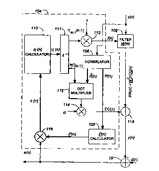
An adaptive filter 100 according to the first embodi
ment of the invention and operating in accordance with
the method described above is shown in Figure 2. It
includes a filter 102 characterized by adaptive filter
coefficients W(n), and means 104 for updating the coeffi
cients, the means being set with a normalized step size a
close to its maximal value, i.e. unity. The filter 102 is
a finite impulse response (FIR) filter which receives a
CA 02318929 2000-07-20
WO 00/38319 PCT/CA99/01068
23
Table 1
Multiply and
Equation accumulate Division
operations
14 2N
15 N
16 N2 1
17 N
18 L
19 L+N-1
20
21 N
22
Total 2L+2Nz+7N-1 1
reference input signal x(n) and an auxiliary signal f(n) (see
Equation (33) below), used for updating the coefficients,
and generates a provisional echo estimate signal PR(n)(see
Equation (3~) below). The updating means 104 includes a
correlator 106 for recursively determining an auto-corre
lation signal presented in the form of auto-correlation
matrix coefficients R(n) based on the reference input sig
nal x(n), and a calculator 108 for generating projection
coefficients P_(n), the projection coefficients being part
of the coefficients of the inverse of the auto-correlation
matrix. The calculator 108 defines projection coefficients
by using an iterative steepest descent method having an
inherent stability of operation as illustrated in detail
above. The projection coefficients are used within updat
ing means 104 for generation the auxiliary filter adapta-
CA 02318929 2000-07-20
WO 00/38319 PCT/CA99/01068
24
tion signal f(n) and an echo estimate correction signal
EC(n) (see Equation (34) below). The latter is used
together with the provisional echo estimate PR(n) to pro-
duce the echo estimate signal y(n).
5 A convention in Fig. 2 is the use of a thick line to
represent the propagation of a matrix or vector signal,
i.e., with more than one component, and the use of a thin
line to stand for a scalar signal propagation. In Fig. 2 a
correlator 106 determines the autocorrelation matrix R(n)
10 in accordance with the Eq. 14 using the current and past
x(n) samples . An "7.~(n) calculator" 110 calculates 1'1(n) based
on Eq: 22, and as shown in Fig. 2, ~(n) is not used by the
updating means 104 until the next sampling interval. The
filter 102 produces the convolutional sum WT(n)X(n). ~N_1(n-1)
15 is obtained from 1>N_1(n) by putting the latter through a
unit delay element 111, providing a delay of one sampling
interval, and further multiplied by the step size a in a
Multiplier 113. The result is used for updating the adap-
tive filter coefficients in (Eq. 18) . ~ (n-1) is dot-multi-
20 plied with part of R(n) by a Dot multiplier 112, and the
result is further multiplied by a multiplier 114 with the
step size oc to form the correction term to be added to
WT(n)X(n) by the summer 116 to form the filter output y(n)
(Equation (19)). The summer. 18 calculates the error, or
f5 the output, e(n), as in Equation (20) . The scalar-vector
multiplier 118 derives ~(n) in accordance with Equation
(21) .
A steepest descent calculator 108 is shown in detail
in Figure 3. Thick lines represent the propagation of a
30 matrix or vector signal, i.e., with more than one compo
nent, and the use of a thin line stands for a scalar sig-
CA 02318929 2000-07-20
WO 00/38319 PCT/CA99/01068
nal propagation. In the calculator 108, the auto-
correlation matrix R(n) and the vector _P(n-1) which is a part
of the estimated inverse of R(n-1), are multiplied in a
Matrix-vector multiplier 130. The vector product is fur-
s ther subtracted by a constant vector [1 0 ... 0]Tin a Sum-
mer 132 to produce the gradient vector g(n), which contains
the feedback error information about using P(n-1) as the-
estimated inverse of R(n). This part corresponds to Equa-
tion (15) . The squared norm of g(n) is then found by dot-
IO multiplying g(n) with itself in a Dot multiplier 134. It is
used as the numerator in calculating ~i(n) in Equation 16. A
Matrix-vector multiplier 136 finds the vector product
between the autocorrelation matrix R(n) and the gradient
vector g(n). This vector product is then dot-multiplied
15 with g(n) in another Dot multiplier 138 to produce the
denominator in calculating (3(n) in Equation (16). This
denominator is reciprocated in a Reciprocator 140, and
then further scalar-multiplied with the aforementioned
numerator in scalar multiplier 142 to produce (3(n). This is
20 the only place where any division operation is performed.
Finally, (3(n) is multiplied with the gradient g(n) in a sca-
lar-vector multiplier 144 to form the correction term to
_P(n-1). This correction term is then subtracted from P(n-1)
in a Vector Summer 146 to derive _P(n) in accordance with
f5 Equation (17) . P(n-1) is obtained from P(n) by using a unit
delay element 148, providing a delay of one sampling
interval.
Two C language prototypes implementing the steepest
descent technique according to the first embodiment of the
invention have been built. The first one, is a floating
point module, and the second one is a 16-bit fixed-point
CA 02318929 2000-07-20
WO 00/38319 PCT/CA99/01068
26
DSP implementation. A floating-point module simulating the
NLMS acoustic echo canceller design in Venture, a success-
ful full-duplex handsfree telephone terminal product by
Nortel Networks Corporation, and a bench mark, floatinq-
5 point module that repeats a prior art FAP scheme by Q. G.
Liu, B. Champagne, and K. C. Ho (Bell-Northern Research
and INRS-Telecommunications, Universite du Quebec), "On
the Use of a Modified Fast Affine Projection Algorithm in
Subbands for Acoustic Echo Cancellation," pp. 354 - 357,
10 Proceedings of 1996 IEEE Digital Signal Processing Work-
shop, Loen, Norway, September 1996, have been also imple-
mented for comparison purposes. The following data files
have been prepared for processing. The source ones are
speech files with Harvard sentences (Intermediate Refer-
15 ence System filtered or not) sampled at 8 KHz and a white
noise file. Out of the source files certain echo files
have been produced by filtering the source ones with cer-
tain measured, 1200-tap, room impulse responses. These two
sets of files act as x(n) and d(n) respectively. The major
20 simulation results are as follows. The bench mark prior
art floating-point FAP scheme with L=1024 and N=5, goes
unstable at 2'57" (2 minutes and 57 seconds, real time,
with 8 KHz sampling rate) with speech training, but with
certain unhealthy signs showing up after only about 25
25 seconds. These signs are in the form of improper excur-
sions of the elements of the vector P(n), first column of
P(n) (inverse of the matrix R(n)) . The fact that it takes
over 2 minutes from the first appearance of unhealthy
signs to divergence, in which period the excursions of the
30 P(n) elements become worse and worse, shows that the coef-
ficient updating algorithm is quite tolerant of certain
CA 02318929 2000-07-20
WO 00/38319 PCT/CA99/01068
27
errors in P(n). Once simulated random quantization noises,
which are uniformly distributed between -0.5 bit and +0.5
bit of a 16-bit implementation, are injected into the
matrix inversion lemma calculation, the prior art~FAP sys
tem diverges in 0.6 second.
For comparison, within the time period of our longest
test case (7'40"), the portions that estimate _P(n), i.e.,-
Eqs. (15)-(17) of the steepest descent scheme of the
invention with the same parameters (L=1024 .and N=5),
always remain stable. Furthermore, the elements in the
vector P(n) progress as expected, without any visible
unhealthy signs like improper excursions during the entire
7'40" period. The output e(n) in the steepest descent
embodiment converges approximately at the same speed as
the bench mark prior art FAP and reaches the same steady
state echo cancellation depth as the prior art FAP and
NLMS. The SFAP according to the first embodiment of the
invention outperforms NLMS filter; with speech training,
it converges in about 1 second while it takes the NLMS
filter about 7 to 8 seconds to do so.
Filters of another length L=512 have also been built
for SFAP, the prior art FAP and NLMS. As expected, they
converge approximately twice as fast as they do for
L=1024 .
Thus, the adaptive filter and method using a steepest
descent calculator for determining the inverse matrix
coefficients, providing a stability of adaptive filtering,
are provided.
A method of adaptive filtering according to a second
embodiment of the present invention uses an iterative
"conjugate gradient" technique to iteratively solve the
CA 02318929 2000-07-20
WO 00/38319 PCT/CA99/01068
28
Equation (10), the corresponding calculator being shown in
Figure 4.
Conjugate gradient is a technique that also seeks the
minimum point of a certain quadratic function iteratively.
Conjugate gradient is closely related to the steepest
descent scheme discussed above. It differs from the steep-
est decent in that it is guaranteed to reach the minimum
in no more than N steps, with N being the order of the
system. That is, conjugate gradient usually converges
faster than the steepest descent. At each iteration (the
same as sampling interval in out application), the conju-
gate gradient takes five steps consecutively:
1. to find the gradient of the quadratic function at
the current point;
2. to find the optimum factor for adjusting the
direction vector, along which adjustment to the parameter
vector will be made;
3. to update the direction vector as determined
above;
4. to find the optimum step size for the parameter
vector updating; and
5. to update the parameter vector as determined
above.
Unlike the steepest descent algorithm, which simply
takes the negative gradient of the quadratic function as
the parameter vector updating direction, conjugate gradi-
ent modifies the negative gradient to determine an opti-
mized direction. By iteratively doing the above, the
scheme reaches the unique minimum of the quadratic func-
tion, where the gradient is zero, in no more than N steps.
The conjugate gradient technique also continuously tracks
CA 02318929 2000-07-20
_ WO 00/38319 PCT/CA99/01068
29
the minimum if it moves, such as the case with non-sta-
tionary input signal x(n). Details about the conjugate gra-
dient algorithm can be found, for example, in a book by
David G. Luenberger (Stanford University), Linear and Non-
linear Programming, Addison-Wesley Publishing Company,
1984.
For an adaptive filtering application, the implied
quadratic function is still shown in Equation (11), whose
gradient with respect to P(n) is also Equation ( 12 ) . Note
that R(n) must be symmetric and positive definite in order
for the conjugate gradient technique to apply, this hap-
pens to be our case. Seeking the minimum, where the gradi-
ent vanishes, is equivalent to solving Equation (10). The
conjugate gradient is also able to track the minimum point
if it moves, such as the case with .non-stationary input
signal X(n) .
Based on the above discussion, the SFAP method
according to the second embodiment, which uses the conju-
gate gradient technique, includes the following steps:
Initialization:
W(0) = 0 , X(0) = 0 , ~(0) = 0 , R(0) = 8I , a = 1 , P(0) _
_ _ l~s
- 0
s(0) = 0 , rsrs(~) = 0 , b(0) = 0
(Equation 24)
Updating the adaptive filter coefficients in sampling
interval n including:
recursive determining of an auto-correlation matrix:
CA 02318929 2000-07-20
WO 00/38319 PCT/CA99/01068
R(n) - R(n- 1)+~.(n)~T(n)-~(n-L)~T(n-L)
(Equation 25)
5 where ~(n) is defined in Equation (23 ) above, and
determining projection coefficients by solving the system
of linear Equations (10) using the conjugate technique,
the projection coefficients being first column coeffi-
cients of the inverse of the auto-correlation matrix:
10 g(n) _ R(n)P(n - 1 ) - 1
0
(Equation 26)
'Y(n) = rsrs(n -1 )gT(n)b(n - 1 )
(Equation 27)
s(n) = y(n)s(n - 1 ) - g(n)
(Equation 28)
b(n) = R(n)s(n)
(Equation 29)
rsrs(n) = 1
sT(n)b(n)
(Equation 30)
a(n) _ -rsrs(n)gT(n)s(n)
(Equation 31)
P(n) _ ~(n -1 ) + (3(n)s(n)
(Equation 32)
CA 02318929 2000-07-20
WO 00/38319 PCT/CA99/01068
31
and performing an adaptive filtering for updating the fil-
ter coefficients
f-f (n) = W(n - 1 ) + a~lN _ 1 (n - 1 )~(n - N) = w(n -1 ) + f(n)X(n - N)
(Equation 33)
y(n) = WT(n)X(n) + a~T(n - 1 )R(n) = PR(n) + EC(n)
e(n) = d(n)-y(n)
(Equation 34)
(Equation 35)
E(n) = e(n)P(n)
'~ (n) _ ~ + E(n)
~(n- 1)
(Equation 36)
(Equation 37)
where R(n) is the first column of R(n), R(n) is an N-1 vector
that consists of the N-1 lower most elements of the N vec-
tor R(n), and ~y(n) is an N-1 vector that consists of the N-1
upper most elements of the N vector ~(n).
The five expressions shown in Equations (26) , (27),
(28), (31) and (32) respectively correspond to the five
steps of the conjugate gradient technique discussed ear-
lier in this section. g(n) is the gradient of the implied
quadratic function, ~y(n) is the optimum factor for updating
the direction vector s_(n). (3(n) is the optimum step size for
parameter vector adjustment, which is made in Equation
CA 02318929 2000-07-20
WO 00/38319 PCT/CA99/01068
32
(32) .
As shown in Table 2,, the total computational require-
ment of the Stable FAP method according to the second
embodiment of the invention is 2L+2N2+9N+1 MACS and 1
division. It should be also ensured that the conjugate
gradient converges fast enough so that the adaptive filter
coeffients converge.
An adaptive filter according to the second embodiment
of , the invention is similar to that of the first embodi
ment shown in Figure 2 except for the calculator 108 now
operating ~in accordance with the conjugate gradient tech-
nique and being designated by numeral 208 in Figure 4.
The conjugate gradient calculator 208 embedded in
the adaptive filter of the second embodiment is shown in
detail in Figure 4. Thick lines represent the propagation
of a matrix or vector signal, i.e., with more than one
component, and the use of a thin line stands for a scalar
signal propagation. In the calculator 208, the autocorre-
lation matrix R(n) and the vector P(n-1), part of the- esti-
mated inverse of R(n-1), are multiplied in a Matrix-vector
Multiplier 210. The resulted vector product is subtracted
by a constant vector [1 0 ... 0]T in a Summer 212 to pro-
duce the gradient vector g(n), which contains the feedback
error information about using P(n-1) as the estimated
inverse of R(n) _ The Matrix-vector Multiplier 210 and the
Summer 212 implement the Equation (26) above. The gradient
g(n) is further dot-multiplied with b(n-1), an auxiliary vec-
tor found in the last sampling interval, in a Dot Multi
plier 214. The resulted scalar product is multiplied by
rs~(n-1) in a Multiplier 216, to produce ~y(n), a factor to be
used in adjusting s(n-1), the direction vector for adjusting
CA 02318929 2000-07-20
_ WO 00/38319 PCT/CA99/OI068
.~
33
P(n-1}.- i'srs(n-1) is obtained from rsrs(n) by putting the latter
through a unit delay element 218, providing a delay of one
sampling interval. Similarly, b_(n-1) is obtained from b(n) by
using another unit delay element 220. The part of the dia-
gram described in this paragraph implements Equation (27)
shown above . With y(n), g(n), and _s(n-1) available, s_(n-1) is
then updated into s(n) by using yet another unit delay- ele-
ment 222, with a delay of one sampling interval, scalar-
vector Multiplier 224 and Vector Summer 226 which imple-
ment operations shown in Equation (28) above. Next, the
auxiliary vector _b(n), to be used in the next sampling
interval, is calculated as the product between R(n) and -_s(n)
in another Matrix-vector Multiplier 230. This implements
Equation (29) above. The vector _b(n) is then dot-multi-
plied with s(n) in yet another Dot multiplier 232, and the
scalar product is reciprocated in a Reciprocator 234, to
produce rsrs(n) (Equation (30) ) . This is where the only divi-
sion operation is. By using yet another Dot Multiplier 236
and a Multiplier 238, g(n) and -_s(n) are dot-multiplied, and
the result, being a scalar product, is multiplied with
-rsrs(n) to derive ~i(n), thus implementing Equation (31)
above. Once (3(n) is available, it is multiplied with s(n) in
another scalar-vector Multiplier 240 to form the correc-
tion term to P(n-1), which is then added to P(n-1) in a Vector
Summer 242 in order to derive _P(n) (Equation (32) above) .
The rest of the structure of the adaptive filter,
employing the conjugate gradient calculator 208, is simi-
lar to that shown in Figure 2 and described above.
CA 02318929 2000-07-20
WO 00/38319 PCT/CA99/01068
34
Table 2
Multiply and
Equation accumulate Division
operations
25 2N
2 6 N2
27 N+1
28 N
2 9 N2
30 N 1
31 N+1
32 N
33 L
3 4 L+N-1
35
36 N
37
Total 2L+2N2+9N+1 1
A C language prototype for 16-bit fixed-point DSP
implementation of the SFAP using the conjugate gradient
scheme has been built and studied. It has the same parame
ters (L=1024 and N=5) and uses same data files as the
steepest descent prototype described above. It behaves
very similarly to its floating-point steepest descent
counterpart. There is no observable difference in the way
_P(n) elements progress, and they also remain stable during
the 7'40" longest test case period. The output e(n) in the
conjugate gradient embodiment converges approximately at
CA 02318929 2000-07-20
WO 00/38319 PCT/CA99/01068
the same speed as the bench mark prior art FAP and reaches
the same steady state echo cancellation depth as the bench
mark prior art FAP and NLMS. The SFAP according to the
second embodiment of the invention also ourperformes NLMS
5 filter in terms of convergence speed. A conjugate gradient
filter of another length L=512 have been also built. As
expected, it converges twice as fast as it does for
L=1024.
A method of adaptive filtering according to a third
10 embodiment of the present invention provides adaptive fil-
tering when the normalized step size has any value from 0
to 1. It updates the adaptive filter coefficients by iter-
atively solving a number of systems linear equations hav-
ing decrementing orders to determine the inverse auto-
15 correlation matrix in a manner described below.
Let's prove first that, if P is the inverse of a sym-
metric matrix R, then it is also symmetric. By definition
RP = I, PR=I
(Equation 38)
Transposing Equation (38) we get
PTRT = IT RTPT = IT
(Equation 39)
respectively. Since R and Iare symmetric, Equation (39)
can be written as
PTR = I , RPT = I
(Equation 40)
CA 02318929 2000-07-20
WO 00/38319 PCT/CA99/01068
36
This means that PT is also the inverse of R. Since the
inverse of a matrix is unique, the only possibility is
PT=P
(Equation 41)
That is, P is symmetric.
Based on the understanding that the inverse of a sym
metric matrix is also symmetric, let's consider a sampling
interval n where we need to find an N-th order square
matrix P(n) so that
R(n)P(n) = I
(Equation 42)
Equation (42) can be written in a scalar form
N- 1
~ rik(n)Pkj(n) = b;~ ~ b'i,j E [0, N-11
k=0
(Equation 43)
where rik(n) is the element of R(n) on row i and column k, and
pkJ(n) the element of P(n) on row k and column j, and di is
defined as
g _ 1, if i=j
0 , otherwise
(Equation 44)
We first solve the set of N linear a
quations defined by
j=0 in Equation ( 43 ) , for (pk0(n), k=0, 1, ..., N-1 } , i . a .
N-1
rik(n)Pk0(n) = si0 ~ ~!1 E [0, N- 1].
k=0
(Equation 45)
Equation (45) coincides with Equation (10) derived earlier
CA 02318929 2000-07-20
WO 00/38319 PCT/CA99/01068
37
and applied to the first and second embodiments of the
invention.
R(n)P(n) - 1
0
(Equation 46)
The right hand side of Equation (45) or Equation (46)_
tells that P(n) is the left-most column of P(n) and, based
on Equation (41) , PT(n) is also the upper-most row of P(n).
According to the first and second embodiments of the
invention :discussed above, this part will cost "2N2+3N"
MACs and 1 division with steepest descent or "2N2+SN+2"
MACS and 1 division with conjugate gradient.
Having dealt with the j=0 case, we now start solving
the set of N linear equations defined by j=1 in Equation
(43) , for {pk~(n),k=0, 1,...,N-1}, i.e.
N- 1
rik(n)pki (n) = Sn , ~/i E [0, N - 1 )
k=0
(Equation 47)
Because P(n) is symmetric so that pp~(n) equals p1~(n), Equa-
tion (47) can be re-arranged to become
N-1
~ r~k(n)Pki (n) = s~ i - r~o(n)Puo(n) ~ di E [0, N _ 1 )
k=1
(Equation 48)
with still N equations but only N-1 instead of N unknowns,
i.e. , {pkl(n), k=1, 2, ..., N-1}, to solve. In general, these N-1
unknowns can be uniquely determined by only N-1 equations.
CA 02318929 2000-07-20
_ WO 00/38319
PCT/CA99/01068
38
Thus, the equation in Equation (48} with i=0 can be omitted
so that it becomes
N-I
rik(n)Pk I (n) = si I - rio(n)plo(n) , t/i E [ l, N _ 1 ]
k=I
(Equation 49)
Equation (49) has the same format as Equation (45) except-
that the order is reduced by one. Equation (49) can also
be solved by using either of the two approaches presented
above, costing "2(N-1)Z+4(N-1) MACs and 1 division with
steepest descent" or "2(N-1)2+6(N-1)+2 MACS and 1 division
with conjugate gradient," where the added "(N-1)" in each
of the two expressions accounts for the extra computations
needed to calculate the right hand side of Equation (49)..
By repeating the above recursion steps, with the
order of the problem decrementing by one each step, we can
completely solve the lower triangle of P(n). Since P(n) is
symmetric, this is equivalent to solving the entire P(n). A
formula for this entire process can be derived from Equa-
tion (43) and the concept described above, as follows:
For j = 0, l, ..., N -1 , solve
N-, si; ~ j = o
rik(n)Pkj(n) = j _ I
k=~
sij - ~, rik(n)pjk(n) ~ 1 <- j 5 N - 1
k=0
b'i E [j, N -1 ]
for { pkj(n), b'k E [j, N-1] ~
(Equation 50)
Note that the right hand sides of Equation (50) for all i
CA 02318929 2000-07-20
WO 00/38319 PCT/CA99/01068
39
at each recursion step j do not contain any unknowns,
i.e., {p~k(n)} there have already been found in previous
stages, Equation (45) and Equation (49) are just special
cases of Equation (50), and {pk~(n), k=j,j+1,...,N-1}
found in recursion step j form a column vector P~(n), which
consists of the lower N-j elements of the j'th (0 <- j < N
1) column of P(n). The process of Equation (50) will take N
divisions and
[2N2 + 3N] + [2(N -1 )2 + 4(N - 1 )] + [2(N - 2)2 + 5(N - 2)] + .:.
+ [2(1)2+(N+2)(1)J
N N N
- ~ [2k2+(N+3-k)kJ = ~ k2+(N+3) ~ k
k=1 k-_1 k-_1
- 6(N+1)(2N+1)+2(N+1)(N+3)= 6N(N+1)(N+2) MACs
(Equation 51)
for steepest descent method, and
N divisions and
[2N2+SN+2]+[2(N-1)2+6(N-1)+2]+[2(N-2)2+7(N-2)+2]+...
+[2(1)2+(N+4)(1)+2]
N N N
- ~ [2k2+(N+5-k)k+2] _ ~ k2+(N+S) ~ k+2N
k-1 k-1 k-1
- 6(N+1)(2N+1)+2(N+1)(N+5)+2N= 6NCN2+ S1N+ Sgl MACs
(Equation 52)
CA 02318929 2000-07-20
WO 00/38319 PCT/CA99/01068
for conjugate gradient method. Note that in deriving Equa-
tions (51) and (52) the following formulae are used
N
k2 -. 6(N+ 1)(2N+ 1)
k=1
5
N
~k = 2(N+1)
x=i
(Equation 53)
which can be easily proven by mathematical induction.
Based on the above derivations, the SFAP method
according to the third embodiment of the invention
includes the following steps:
Initialization:
w(0) = 0 , ~(0) = 0 , r~(0) = 0 , R(0) = 8I , e(0) = 0 , P(0) _
l~s
- 0
(Equation 54)
Updating the adaptive filter coefficients in sampling
interval n including the steps shown in Equation 55 below.
Please, note that designations used in Equation (55), are
as follows: ~(n) is defined in Equation (23} above, R(n) is
the first column of R(n), R(n) is an N-1 vector that con
sists of the N-1 lower most elements of the N vector R(n),
and ~(n) is an N-1 vector that consists of the N-1 upper
most elements of the N vector ~(n). Please, also note that
any division operation in the 2nd expression of Equation
(55) is not performed if the denominator is not greater
than zero, in which case a zero is assigned to the quo-
tient.
CA 02318929 2000-07-20
WO 00/38319 PCT/CA99/01068
41
MAC IDivi;
T
R(n) =
R(n
-
I
)
+
~(n)~
(n)
- 2N
~(n
-
L)~T(n
-
L)
~.- ~ 6N(N + 1 )(N
'~~ + 2)
~
'
Recursion
with
decrementing
order (Steepest descent)
t to
do
matrix
inversion
P(n) = R or N
(n)
8
NCN2 +
N +
6
5
5
J
(Conjugate gradient)
W(n) = L
w(n
_
I
)
+
a~ltv
_
t
(n
-
I
)X(n
_
N)
y(n) = WT(n)X(n) L + N - 1
+
allT(n
-
I
)R(n)
e(n) = d(n)
-
y(n)
e(n) = e(n) N - I
( I
- a)e(n
- 1
)
~(n) = P(n)e(n) N2
~ (n) ~ +
E(n)
I )
,~ (
2L+6N3+2N2+ 3 N-2
(Steepest descent)
Total or N
2L + SN3 + 9N2 + 26N - 2
6 2 3
(Conjugate gradient)
(Equation 55)
An adaptive filter 300 according to a third embodiment of
the invention, shown in Figure 5, is similar to that of
Fig. 2 with like elements being designated by same refer-
CA 02318929 2000-07-20
WO 00/38319 PCT/CA99/01068
42
ence numerals incremented by 200. The filter 300 also dif-
fers from the filter 100 by the following features: the
normilized step size may have any value from 0 to 1.0, the
calculator 308 now has more extended structure for consec-
utively determining columns of the inverse auto-correla-
tion matrix in accordance with the steepest descent
technique, and an e(n) calculator 320 is added.
The P(n) calculator 308, now being a matrix calcula
tor, operates in accordance with the flow-chart 400 shown
in Figure 6_ Upon start up for the sampling interval n
(block 401), the routine 402 sets an initial value to
index j (block 404) which is submitted together with the
auto-correlation matrix R(n) (block 406) to a projection
coefficient column calculator (block 408). The calculator
provides a steepest descent iteration in accordance with
Equation (50) for the current value of index j, thus updat-
ing the corresponding column of projection coefficients
from the previous sampling interval (block 408). The
updated column of the projected coefficients is sent to a
storage means (routine 410, block 412) to be stored until
the other columns of P(n) are calculated. Until the index j
is equal to N-1 (block 416), its value is incremented by 1,
i.e. made equal to j+1 (block 418), and the steepest
descent iteration is repeated (block 408) to determine the
next column of P(n). By performing N corresponding steep-
est descent iterations for j = 0, 1, ... N-1, all columns of the
inverse auto-correlation matrix are thus determined and
assembled into P(n) in an assembling means (block 414). A
command/signal (block 420) then notifies about the end of
the sampling interval n and the beginning of the next sam-
pling interval n+1 where the steps of the routine 400 are
CA 02318929 2000-07-20
WO 00/38319 PCT/CA99/01068
43
repeated. In Figure 6, thick lines represent the propaga-
tion of a matrix or vector signal, i.e., with more than
one component, and the use of a thin line stands for a
control propagation.
In modification to this embodiment, the steepest
descent calculator 308 may be replaced with the conjugate
calculator. The corresponding structure is illustrated by
a flow-chart 500 shown in Figure 7 where the blocks simi-
lar to that ones of Figure 6 are designated by same refer-
ence numerals incremented by 100. It operates in a manner
described above with regard to Figure 6.
A method of adaptive filtering according to a fourth
embodiment of the present invention also provides adaptive
filtering when the normalized step size has any value from
0 to 1. It updates the adaptive filter coefficients by
iteratively solving a number of systems linear equations
which avoid an explicit matrix inversion performed in the
third embodiment of the invention. The details are
described below.
The second equation from the set of Equations (6),
which is reproduced for convenience in Equation (56)
below, is equivalent to
R(n)~(n) _ _e(n)
(Equation 56)
It is possible to obtain ~(n), required for updating the
adaptive filter coefficients, directly from the set of
linear Equations (56), which are solved again by one of
the descending iterative methods.
As a way of example, we will use a conjugate gradient
method. and perform N conjugate gradient iterations so that
an exact solution, not an iterated one, is reached. It is
CA 02318929 2000-07-20
WO 00/38319 PCT/CA99/01068
44
ensured by the fact that the, conjugate gradient method is
guaranteed to reach the solution in no more than N itera-
tions, with N being the order of the problem, see Equation
(55) . It is convenient to start with Vi(n)=0 before itera-
tions begin at each sampling interval n to save some com-
putation time.
Accordingly, the SFAP method of the fourth embodiment
of the invention includes the following steps:
Initialization: MAC Divisio
E~(0) = 0 , s(0) = 0 , rsrs(0)
= 0 , b(0) = 0
In sampling internal n, repeat
the following
equations N times, i.e., for
k = 0,1, ..., N-1:
g R(n)~'(k) e(n) ( N- 1) x N2
'Y = rsrs(k)gTl?(k) (N - I ) x
(N + I )
s(k+ 1) _ ~ys(k)-g ( N- 1) xN
b(k + 1 } = R(n)s(k + 1 )
2
N x N
rsrs(k + 1 ) = I
s(k+ 1)Tb(k+ 1) NxN Nx 1
~ _ -rsrs(k+ I)gTS(k+ 1) Nx (N+ 1)
~~(k + 1 ) = Ei(k) + /3s(k +
I ) NxN
2~
Output:
~(n) _ c(N)
Total 2N3 + 4Nz -1 N
(Equation 57)
CA 02318929 2000-07-20
WO 00/38319
PCT/CA99/01068
The steps of the adaptive filtering methods according
to the fourth embodiment are presented in more detail
below:
Initialization:
5 l~s
w(o) = o , x(o} = o , ~(o) = o , R(o) = sl , ~(o) = o , P(o}
o
(Equation 58)
Processing in sampling interval n:
MAC Division
R(n) =
R(n
-
1
)
+
~(n)~T(
n)
- 2N
~(n
-
L)~T(n
-
L)
W(n) = L
W(n-1)+arlN_~(n_1)X(n-N)
y(n} = L + N- 1
wT(n)X(n)
+
a~T(n
-
1
)R(n)
N
e(n} =
d(n)
-
y(n)
e(n) =e(n)
( 1 - N conjugate N -1
a)e(n
- 1
)
2 0 gradient
(,_.___..._.___
iterations
._____......__..___.
.._.._._.__.._____._._.._._...________..........__..
Solve R(n)E(n) N3
= 2
e(n)
for
~(n)
;
2
+ 4N
c~~;~r - 1
~ (n) ~
+
(n)
t~(n-
1)
Total I 2L + 2N3 + 4N2 + 4N - 3 ~ N
(Equation 59)
where the designations are similar to that presented with
regard to the first, second and third embodiments
CA 02318929 2000-07-20
WO 00/38319 PCT/CA99/01068
46
described above. Note that any division operation in Equa-
tion (56) is not performed if the denominator is not
greater than zero, in which case a zero is assigned to the
quotient.
An adaptive filter 600 according to a fourth embodi-
ment of the invention is shown in detail in Figure 8. It
includes a filter 602 characterized by adaptive filter-
coefficients W(n), and means 604 for updating the coeffi-
cients, the means being set with a normalized step size a
having any value in a range from 0 to 1Ø The filter 602
is a finite impulse response (FIR) filter which receives a
reference input signal x(n) and an auxiliary signal f(n)
used for updating the coefficients, and generates a provi-
sional echo estimate signal PR(n). The updating means 604
includes a correlator 606 for recursively determining an
auto-correlation signal presented in the form of auto-cor-
relation matrix coefficients R(n) based on the reference
input signal x(n), an ~(n) calculator 608 and an e(n) calcula-
tor 620 for corresponding calculation of vectors ~(n) and
e(n). The calculator 608 defines ~(n) by using an iterative
conjugate gradient method having an inherent stability of
operation as illustrated in detail above. The projection
coefficients are used within updating means 604 for gener-
ation the auxiliary filter adaptation signal f(n) and an
echo estimate correction signal EC(n). The latter is used
together with the provisional echo estimate PR(n) to pro-
duce the echo estimate signal y(n). In Fig. 8 thick lines
represent propagation of a.matrix or vector signal, i.e.,
the signal with more than one component, and the use of a
thin line stands for a scalar signal propagation. In Fig.
8 a correlator 606 determines the autocorrelation matrix
CA 02318929 2000-07-20
WO 00/38319 PCT/CA99/01068
47
R(n) in accordance with the first formula of Eq. (59) using
the current and past x(n) . samples . An ~~~(n) calculator" 610
calculates ~(n) based the last formula of Eq. (59), and as
shown in Fig. 8, ~(n) is not used by the updating means 104
until the next sampling interval. The filter 602 produces
the convolutional sum WT(n)X(n) . ~N_1(n-1) is obtained from
'~~_1(n) by putting the latter through a unit delay element-
611, providing a delay of one sampling interval, and fur-
ther multiplied by the step size a in a Multiplier 613.
The result is used for updating the adaptive filter coef-
ficients (Eq. 59, second formula) . ~(n-1) is dot-multiplied
with part of R(n) by a Dot multiplier 612, and the result
is further multiplied by a multiplier 614 with the step
size a, to form the correction term to be added to WT(n)X(n)
by the summer 616 to form the filter output y(n) (Equation
(59) , third formula) . Signals y(n) and e(n) are further sent
to the e(n) calculator 620 to determine e(n) in accordance
with a fourth and fifth formulae of Equation (59), and the
results are sent to the ,~(n) calculator 608 together with
the auto-correlation matrix R(n) derived in the correlator
606. The ~(n) calculator 608 solves the sixth equation of
Eq. (59) for ~(n) by a conjugate gradient method, thus pro-
viding sufficient data for updating the adaptive filter
coefficients (Eq. 6, first formula).
The ~{n) calculator 608, shown in detail in Figure 9,
includes a one-step calculator 708a similar to the calcu-
lator 208 of Fig. 4 and includes like elements which are
referred to by the same reference numerals incremented by
500 respectively (except for P n-1 and ~ being replaced
with ~(n-1) and ~(n) respectively) . Thick lines represent the
propagation of a matrix or vector signal, i.e., with more
CA 02318929 2000-07-20
WO 00/38319 PCT/CA99/01068
48
than one component, and the use of a thin line stands for
a scalar signal propagation. At each sampling interval n,
the calculator 708a performs N steps corresponding to k = 0,
1, ... N-1, each step being similar to the conjugate gradient
iteration performed by the filter 208 of the second embod-
iment of the invention. The calculator 608 additionally
includes an output switch 754 which automatically opens-
at the beginning of the sampling interval and closes at
the end of N conjugate gradient iterations.
IO Modifications described with regard to the first two
embodiments are equally applicable to the third and fourth
embodiments of the invention.
Two "C" prototypes according to the third and fourth
embodiments of the invention have been implemented in a
floating point PC platform. They have demonstrated results
completely consistent with the results of the first and
second embodiments of the invention.
Thus, an adaptive filter and a method providing a sta
bility of adaptive filtering based on feedback adjustment,
are provided.
Although the methods operate with real-valued num-
bers, it does not prevent the invention from being
extended to cases where introduction of complex numbers is
necessary.
Although the embodiments are illustrated within the
context of echo cancellation, the results are also appli-
cable to other adaptive filtering applications.
Thus, it will be appreciated that, while specific
embodiments of the invention are described in detail
above, numerous variations, modifications and combinations
CA 02318929 2000-07-20
WD 00/38319
PCT/CA99/01068
49
of these embodiments fall within the scope of the inven-
tion as defined in the following claims.
10
20
30