Note: Descriptions are shown in the official language in which they were submitted.
CA 02386568 2002-05-15
System for Estimating Azimuthal Variations in Seismic Data
BACKGROUND OF THE INVENTION
1. Field of the Invention
This invention is related to seismic data processing. More specifically, the
invention is related to a system for processing seismic data to detect
azimuthal velocity
variations.
2. Description of Related Art
Seismic surveys are routinely used in the search for oil and gas reservoirs in
the
earth's subsurface. Seismic surveys are performed by imparting acoustic energy
into the
earth, either at a land surface or in a marine environment, and then detecting
the
reflected and refracted acoustic energy. The delay time between the imparting
of the
acoustic energy wave at the source location and detection of the same wave at
a receiver
location indicates the depth of reflecting geological interfaces.
Until recently, only two-dimensional ("2D") seismic surveys were conducted,
with the seismic source locations being collinear with a line of receivers.
Recent
advances in technology have enabled three-dimensional ("3D") seismic survey
data to be
gathered and analyzed. Typically, in 3D surveys arrays of seismic receivers
are deployed
which receive reflected acoustic energy imparted at varying locations that may
be
specifically selected to provide a rich assortment of azimuths for common
midpoints.
A technique frequently used in seismic survey analysis is AVO analysis, which
is
the amplitude variation with offset, and is also referred to herein as
amplitude variation
with incidence angle. According to the AVO approach, attributes of a
subsurface
interface are determined both from the normal-incidence amplitude of reflected
seismic
energy, and also from the dependence of the detected seismic reflections on
the angle of
incidence of the seismic energy at a subsurface reflecting interface relative
to the
vertical. In conventional AVO analysis, multiple seismic traces having a
common
-1-
AXG-001
CA 02386568 2002-05-15
reflection point, commonly referred to as a common mid point or common depth
point(CMP or CDP) gather, are collected. From the CMP (or CDP) gather, one may
derive the amplitude R of a reflected seismic wave from an interface (i.e.,
the "target
horizon") as a function of the angle of incidence e from the normal according
to the
following relationship:
R(0) = A + B sin' 0
In this case, the coefficient A is the zero-offset response (also referred to
as the AVO
intercept), while the coefficient B is referred to as the AVO slope, or
gradient, as it is
representative of the rate of change of amplitude with the square of the angle
of
incidence. Analysis of the AVO slope and intercept can provide indicators of
interesting
formations, from an oil and gas exploration standpoint. For example,
variations in the A
and B values from a theoretical A-versus-B trend line for the expected
stratigraphic
sequences can indicate the location of hydrocarbon reserves.
While simple models of subsurface geology assume azimuthal isotropy in the
propagation of acoustic energy it has been observed that azimuthal anisotropy
is in fact
present in many survey regions, such that the velocity of acoustic energy
depends upon
the azimuth of the source-receiver path. lf azimuthal anisotropy is present,
the
conventional normal moveout correction may not adequately align the seismic
traces in
the gather, which can result in degraded AVO analysis.
Normal moveout correction of the seismic data, both for offset-dependent
delays
and also for azimuthal anisotropy caused by the overburden, is therefore
typically
performed in producing stacked traces of improved signal-to-noise ratio for
use in a 3D
seismic survey. For example, U. S. Patent No. 5,532,978 describes a method of
deriving and applying azimuthal anisotropy corrections to seismic survey
signals.
The detection of a preferred azimuthal direction at a reflecting interface can
also
provide important information regarding geological features. For example, a
preferred
azimuthal reflection direction can indicate the presence of aligned vertical
fractures. For
moderately far offsets (250- 350 incidence angles), the P-wave traveling in
the plane
-2-
AXG-001
CA 02386568 2002-05-15
wave parallel to aligned vertical fractures has a higher velocity than the P-
wave traveling
in the plane perpendicular to the fractures.
Traditionally, azimuthal velocity analysis has been performed using azimuth-
sectored supergathers and picking semblance maxima at various azimuths. This
reduces
the problem to a series of 2-D solutions, rather than solving the complete 3-D
solution.
In some cases as few as two sectors may be chosen, perpendicular and parallel
to the
(average) principal axes of the azimuthal anisotropy. If more than two sectors
are used,
an ellipse is fitted to the picked velocities to give fast and slow velocity
magnitudes and
the azimuth of the fast velocity. These procedures suffer from several
drawbacks:
Picking semblance, by hand, on azimuth sectored data is processor/interpreter
dependent and extremely time consuming.
Semblance works well fbr data which do not show amplitude variation with
offset ("AVO"), however, if the data contain significant AVO, particularly if
there is a
polarity reversal, semblance can fail. In this case automatic picking of
semblance
maxima will be erroneous.
If the subsurface has azimuthal velocity variation ("AVV") then this will
appear
as an offset-dependent static viewed on offset-sorted CMP gathers. This will
reduce the
effectiveness of any surface consistent statics solution, thus the azimuth-
sectored
supergathers will most likely be contaminated with statics. This will
significantly
degrade the semblance analysis and may result in several semblance maxima.
The semblance is based on giving the greatest stack power. However, for AVV
analysis it is the actual subsurface velocity that is of interest, not simply
the velocity that
gives the best stack. For instance, if a higher amplitude occurs at a
particular azimuth
within the sector, then the velocity at that azimuth will be picked. In
addition, if those
high amplitudes are at the mid to near offsets and are contaminated with
residual statics
then a completely erroneous velocity could give the highest semblance.
-3-
AXG-001
CA 02386568 2002-05-15
Sectoring and partial stacking of the data means that it is extremely
difficult to
obtain error estimates. Not only is it difficult to attribute a picking error
from picking
semblance, but errors due to the acquisition geometry are not represented. In
any
analysis of this type it is important to compute the errors associated with
the obtained
results. For instance a weighted least squares approach has been used to
compute the
errors in a technique for inverting azimuthal variation of amplitude for shear
wave data.
It has also been observed that the reliability of the amplitude variation with
azimuth
analysis has been assessed by looking for an absence of the acquisition
geometry being
mirrored in the anisotropy maps.
It should be noted that the description of the invention which follows should
not
be construed as limiting the invention to the examples and preferred
embodiments
shown and described. Those skilled in the art to which this invention pertains
will be
able to devise variations of this invention within the scope of the appended
claims.
SUMMARY OF THE INVENTION
The invention comprises a system for processing seismic data to estimate time
shift resulting from velocity anisotropy in the earth's subsurface. A gather
of seismic
data traces is formed and selected seismic data traces included in said gather
within
selected time windows are cross-correlated to estimate the time shift in the
seismic data
traces included in said gather resulting from velocity anisotropy in the
earth's
subsurface.
BRIEF DESCRIPTION OF THE DRAWINGS
FIG. 1 shows a simplified portion of a 3D seismic source-receiver layout for a
3D seismic survey.
-4-
AXG-001
CA 02386568 2002-05-15
FIG. 2A shows representative seismic data traces from a common midpoint
gather prior to application of normal moveout adjustment.
FIG. 2B shows the seismic data traces shown in FIG. after application of
normal
moveout adjustment.
FIG. 3 is a flow chart showing an embodiment of the invention.
FIG. 4 is a flow chart showing a further embodiment of the invention.
FIG. 5 is a flow chart showing a further embodiment of the invention.
FIG. 6 is a flow chart showing a further embodiment of the invention..
FIG. 7 is a flow chart showing a further embodiment of the invention.
FIG. 8 is a diagram illustrating a spatial relationship of the invention.
FIG. 9 shows a computer system for carrying out the invention.
DESCRIPTION OF PREFERRED EMBODIMENT
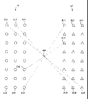
FIG. 1 shows a simplified portion of a 3D seismic source-receiver layout for a
3D seismic survey. Shown in FIG. 1 is a portion of a receiver array 12,
positioned on
the earth's surface, comprising three columns of receivers, with each column
including
eight receivers. Source array 14 includes a group of source locations.
Typically, a
seismic source is moved along the surface of the earth, and the source is
activated at
specific source locations in a sequence. The acoustic energy imparted at each
source
location travels through the earth and, after reflection from subsurface
geologic
interfaces, is detected by each receiver in the receiver array.
Also shown in FIG. 1 is an example of a common midpoint MP. The common
midpoint shown is common to several source receiver paths in this survey. FIG.
1
illustrates MP as being a midpoint between source location Sll and receiver
location
R38; source location S21 and receiver location R28; source location S38 and
receiver
location R11; and source location 536 and receiver location R13. It will be
apparent to
those of ordinary skill in the art that location MP could be the common
midpoint for a
-5-
AXG-001
CA 02386568 2002-05-15
large number of source-receiver pairs, and also that there are a large number
of common
midpoints between other source receiver pairs. Each of these source-receiver
paths may
be of a different length (offset) and different direction (azimuth). Although
common
mid point gathers are typically used in implementing the present invention, if
the
subsurface strata are dipping rather than flat, additional processing known to
those of
ordinary skill in the art may be performed on the seismic data to develop
common
reflection point gathers to which the present invention may be applied.
As is well known in the art, normal moveout corrections are typically made to
traces in a common midpoint gather to correct for the additional delay time
for longer
offset traces, so that the travel time of each seismic signal is effectively
normalized to a
zero-offset travel time. In situations where the earth exhibits no azimuthal
anisotropy,
the azimuthal variation will not introduce a variation in the data set.
However, when
azimuthal anisotropy is present in seismic survey signals, the standard normal
moveout
correction may not adequately correct for variations in delay times for traces
from
source-receiver pairs of different directions.
Variations in the seismic data traces will appear to be variations in
amplitude as a
function of the azimuthal variation, when in reality the variations in the
seismic data
traces are a result of azimuthally dependent time shifts. A velocity variation
with
azimuth of only a few percent can cause ten milliseconds or more of time
difference in
the location of an event in a seismic data trace. Accordingly, velocity
variations below
the resolution of conventional semblance based velocity analysis can distort
the
amplitude variation with incidence angle (AVO) and the amplitude variation
with
azimuth ("AVOA"), resulting in an incorrect computation.
In addition to the standard normal moveout correction, typically, for 3-D land
acquisition, deconvolution, refraction statics, and two passes of surface
consistent
residual statics processes are applied to the data. As a preliminary to the
performance of
the invention as disclosed herein, noise reduction, trace scaling and any
other single-
-6-
AXG-00 1
CA 02386568 2002-05-15
trace process may be applied, however, the application of multi-trace
processing should
be avoided.
FLATTEN EVENTS WITHIN A MOVING TIME WINDOW
If the velocity of the seismic signals in the subsurface vary with the
azimuthal
direction in which the seismic signals travel, the conventional normal moveout
correction will not align the traces properly, and in accordance with a
preferred
embodiment of the invention, the following process may be utilized to achieve
proper
trace alignment. FIG. 2A and FIG. 2B show representative traces from a common
midpoint gather. An initial velocity profile for the seismic traces may be
generated in a
conventional manner and normal moveout applied to the traces. FIG. 2A shows
the
traces prior to applying normal moveout adjustment to the traces and FIG. 2B
shows
these same traces after application of the normal moveout adjustment. As
outlined in
FIG. 3, and with reference to FIG. 2B, in a preferred embodiment of the
invention a first
time window is selected in step 50. Time windows utilized for performing the
invention
may typically be in the range of 100 to 300 milliseconds, however, the time
window
utilized may vary in accordance with the judgment of the processor. A first
selected
time window for the data shown in FIG. 2B may extend from 500 milliseconds to
700
milliseconds. In step 52, a spatial window comprising a number of spatially
related
traces is selected and the traces in this spatial window are summed together
within the
selected time window to create a "pilot" trace. In step 54, one trace is
selected from the
pilot trace, which will be referred to as the "input" trace. In step 56 the
summed pilot
trace is cross-correlated with the input trace within the selected time window
and in step
58 the time shift between the input trace and pilot trace which yields the
maximum
correlation is determined and recorded.
The spatial window is then moved across the CMP gather within the selected
time window by one trace and a new pilot trace is generated for this new
spatial
window. The new pilot trace is then correlated with the new input trace within
the time
window. This process is continued for the selected time window, with each
successive
data trace within the gather being designated as the "input trace" and cross-
correlated
-7-
AXG-001
CA 02386568 2002-05-15
with a pilot trace which comprises a plurality of nearby traces, to complete a
time
window trace correlation sequence. In this way the pilot trace represents the
local phase
and amplitude characteristics of the data for each "input" trace. Accordingly,
a decision
is made in step 60 as to whether a time window trace correlation sequence has
been
completed. If the answer is no, steps 52, 54, 56, 58 and 60 are repeated for a
successive
input trace. If the answer is yes, then in step 62 a decision is made as to
whether the
cross-correlation sequence just completed is the first performed cross-
correlation
process for the time window. In one implementation of the invention, if the
answer is
yes, the calculated time shift that provided maximum cross-correlation between
the input
trace and the pilot trace for each trace is applied to each trace in step 64
and steps 52,
54, 56, 58, 60 and 62 are repeated. If the answer in step 62 is no, then in
step 66 a
decision is made as to whether any reflection event in the time window is
substantially
aligned across the traces in the gather. If the answer is no steps 64, 52, 54,
56, 58, 60,
62 and 66 are repeated. This decision in step 66 is normally based on whether
or not the
additional time shifts calculated for the input traces in the just completed
time window
trace correlation sequence are significant. If the answer in step 66 is yes,
then in step
68, the total computed time shifts for each trace are stored and the traces
are returned to
their form they were in prior to beginning the process outlined in FIG. 3.
Typically, only
two iterations of the process described in steps 52, 54, 56, 58, 60, 62 and 64
are
performed, but further iterations; may be performed if, in the judgment of the
processor,
data quality may be improved by further iterations.
A decision is made in step 70 as to whether all time windows of interest in
the
seismic data gather have been selected, and if the answer in no a new time
window is
selected in step 50 and the cross-correlation procedure described above with
respect to
steps 52, 54, 56, 58, 60, 62 64, 66, 68 and 70 is repeated for all time
windows of
interest. The successive time windows selected may occupy successive time
positions
on the seismic data traces or the time windows may overlap, depending on the
quality of
the data.
-8-
AXG-001
CA 02386568 2002-05-15
Following completion of the cross-correlation procedure for all time windows
and all traces within each time window, in step 72, the amount of time shift
which
achieved the maximum correlation for each trace within each time window is
applied to
each trace at the center point within each time window, and, in step 74, time
shifts for
the remainder of the data traces are interpolated between these center points.
Each pilot trace may comprise, for example, eleven traces. The trace in the
center of the selected spatial window, i.e. the sixth trace, may be designated
as the
"input" trace and cross-correlated with the pilot trace to obtain a time
shift. The spatial
trace window is then moved one trace across the gather and a new pilot trace
formed.
Again, the trace in the center of this window, i.e. the next trace in the
gather, is
designated as the "input" trace and cross-correlated with the pilot trace to
obtain a time
shift for that trace. At the edges of the gather, in this example the first
through the sixth
traces, the spatial window comprising the pilot trace may be shortened so
that, if the
first trace is the "input" trace, the first through sixth traces are stacked
to form the pilot
trace, and for the second trace, the first through the seventh traces are
stacked and so
on, until the full number of traces desired in the spatial window is reached
(in this
example, eleven). The number of traces selected to form the pilot trace may be
selected on the basis of the magnitude of amplitude variation with offset in
the data and
the magnitude of noise such as multiple contamination.
In performing the cross-correlation procedure, amplitude and phase variations
with offset, including the case where an event reverses polarity at some
offset are taken
into account. The pilot trace represents the "local" data characteristics. If
an event
reverses polarity at far offsets then the pilot trace at near offsets should
not include the
far offset traces. Similarly, the pilot trace at far offsets will not include
traces at near
offsets.
Other trace attributes, including absolute values, RMS values, or trace
envelope
may be used for performing the cross-correlation in addition to the raw trace
reflection
amplitude.
-9-
AXG-001
CA 02386568 2002-05-15
At such time as the time shifts have been applied to the seismic data traces
in the
gather, AVO analysis as well as AVOA analysis, such as discussed herein with
reference
to FIG. 4, may be performed on the adjusted traces.
COMPUTING THE AMPLITUDE VARIATION WITH INCIDENCE ANGLE
(AVO), AND THE AMPLITUDE VARIATION WITH AZIMUTH (AVOA)
It is known to those of ordinary skill in the art that amplitude variation
with
incidence angle (also referred to as amplitude variation with offset), as well
as the
amplitude variation with azimuth for a reflection from a horizontal transverse
isotropic
layer of the earth which is overlain with an isotropic overburden can be
approximated by
the following equation:
R(0,0) = 1+ GISin: (8) + G2Sin2 (0)Cos2 (0 - fl)
(Eq. 1)
where: R(0,0) is the reflection coefficient as a function of 8 , the incidence
angle of
the seismic energy at a subsurface reflecting interface relative to the
vertical, and
0 , the receiver azimuth with respect to a predefined zero azimuth direction
(for
example, true north);
/ is the P-wave impedance contrast between the subsurface layers from which
the signal is reflected;
G/ is the isotropic AVO gradient;
G2 is the azimuthal or anisotropic term; and
)8 (with reference to FIG. 8 ) is the angle between the predefined zero
azimuth
direction (such as true north) and the maximum AVO gradient direction.
-10-
AXG-001
CA 02386568 2002-05-15
G1 and G2 are given by:
A V ( \ 2 /
1 A V, A p\
G, - -
- 2 ¨ + ,
(Eq. 2)
2 V g V, P
and
(
1 \ 2
G2 = A + 2 ¨ A ,
(Eq. 3)
\ gi
where: Ap, A Vp and A Vs are the change in density, the change in P-wave
velocity,
and the change in S-wave velocity, respectively,
p ,Vp and V, are the average density, the average P-wave velocity and the
average S-wave velocity respectively,
g= the average P-wave velocity divided by the average S-wave
velocity,
A (v) is the change in 8(v) across the reflecting boundary, and
A 7 is the change in the shear wave splitting parameter 7 across the
reflecting
boundary, where:
C1212 - C3232
¨
2C33
It is known to those of ordinary skill in the art that for a linearly elastic
material, each
component of stress au is linearly dependent on every component of strain eki,
where
, j, k and / are directional indices that may assume values of 1, 2 or 3. The
stress-
strain dependency is given by Hooke's Law:
a- = Cyklekl
-ii-
AXG-001
CA 02386568 2002-05-15
where Cyk/ is the elastic modulus tensor and completely characterizes the
elasticity of
the medium. The relationship between (v) and the elastic modulus tensor is
given
by:
C
( - ,
(5.(v) 11.).3 Ci232 2 - ( ,3333 c3232 )2
2 C3333 ( C3333 - C3232 ) 2
However, without knowing fl , Eq. 1, cannot be solved using a least squares
approach. However, Eq. I can be rewritten as:
R(0,0) = 1+ IG1 + G2Cos2 (0 - 13)1 Sin2 (0)
(Eq. 4)
which can be rewritten as:
R(0,0) = I + IG1* + (G2* - GI* )Cos2 (0 - fl)}Sin2 (0)
(Eq. 5)
so that GI = G1* and G2 = G2 - G1*.
Utilizing the equality:
G1* + (G2* - GI* )Cos2 (0- /3)=G2* COS2 (0 - fi) + G,* Sin2 (0 - fi) (Eq. 6)
then
R(0, 0) = 1+ [G2 *Cos2 (0 - fl) + G,* Sin2 (0 - /6]Sin2 (0).
(Eq. 7)
It is known to those of ordinary skill in the art that:
*Cos2 (0 - ,8)+ GI" Sin2 (0 - fi) =
Wi1Cos2 (0) + 2W12Cos(0)Sin(0) + W
22Sin2 (0) (Eq. 8)
which is linear in the unknowns WI, , W12 and J4'13, which can be related back
to the
unknowns G,*, G2* and /3, as follows:
G2* = 115(W11 + W22 + V(WI 1 - W,2)2 + 4W2 2 )
(Eq. 9)
GI*= (15(Wi + W22 V(WII - W22)2 + 4W2 2 )
(Eq. 10)
-12-
AXG-001
CA 02386568 2002-05-15
- W22 4- \kW!! - W22)2 + 4W122
= ATAN _______________________ 2
(Eq. 11)
Wi2
Thus, combining Equations 1 with Equations 4 -11, Equation 1 can be written
as:
R(0,0) = 1 +[WilCos2 (0) + 23'12Cos(0)Sin(0)+ W
22Sin2 (0)]Sin2(0)Eq. 12)
with
G1 = 0-5(WI + W22 - NAW11 - W22)2 + 4W122 (Eq. 13)
G = (W W )2 4W22
2 11 22
(Eq. 14)
and
PV22 V(Wli ¨ 2) +422)
,5 = ATAN (Eq. 15)
2w12
Values of the reflection coefficient R(t 9 ,0) for specific values of the
incidence
angle 8 and the source-receiver azimuth 0 can be obtained from the recorded
seismic
data for each reflection event by extracting the amplitudes of the seismic
data traces as a
function of offset and azimuth. With reference to FIG. 4, in step 80, values
of the
reflection coefficient R(0,0) and the source-receiver azimuth 0 are obtained
from the
seismic data that is being processed. To obtain the value of an incidence
angle 0 , a
smoothed version of the interval velocity is calculated in step 82 in a manner
well known
to those of ordinary skill in the art, and the RMS velocity is computed in
step 84 from
-13- AXG-001
CA 02386568 2002-05-15
the smoothed version of the interval velocity. In step 86, the values of the
incidence
angle, 0 , may then be determined, utilizing the following equation:
X
0 = ASIN{ _____________ Vint ____________________________________________
(Eq. 16)
Vms. x 2 + To2 vrms2
where:
X is the source to receiver offset;
To is the zero offset two way travel time;
Vr., is the RMS velocity; and
Vint is the interval velocity at the time of interest.
In step 88, a least squares method is used to compute reflection coefficient
as a function
of azimuthal angle and incidence angle for the seismic traces comprising the
CMP
gather. Eq. 12 is solved in a straightforward least squares manner, known to
those of
ordinary skill in the art, for the unknowns, I , WI 1 , W22 , and r+2. Values
for G1 (the
isotropic AVO gradient), G2 (the azimuthal or anisotropic term) and i0 may
then be
computed from values computed for J471, W2. and W
2 . Accordingly, it is
demonstrated that Eq. 1 is linear in I, GI, G2 and the direction /1.
Note that as indicated above in Eqs. 2 and 3, the derived gradients G1 and G2
AV AV fr Ap
are related to physical rock properties ¨ , P , , A so" and Ay .
V
Vs Vs
COMPUTING THE AZIMUTHAL VELOCITY VARIATION (AVV)
Because the process outlined in FIG. 3 determines the time shift in seismic
traces
associated with the azimuthal velocity variation, this determined time shift
information
may be used to compute the actual azimuthal velocity variation. Steps for
computing
-14-
AXG-001
CA 02386568 2002-05-15
the azimuthal variation of velocity are outlined in FIG. 5. In step 90 the
total travel
time T for each trace is computed by adding the time shifts determined in the
process
described with reference to FIG. 3 which achieved maximum correlation for each
trace
and the time shift obtained as a result of standard NMO correction to To , the
zero
offset travel time. The following equation may then be utilized to solve for
the
azimuthal velocity variation:
X2
T2 _ T2 + __________________
(Eq. 17)
Vnmo2 (0 )
where:
T = total travel time
To = two way zero-offset traveltime
X = offset
V. (0 ) = the azimuthally varying velocity as a function of the azimuth 0,
and
1
__________________________________________________________________________ ¨ W
Cos2(0) + 2W12Cos(0)Sin(0)+ W22 Sin2 (0) (Eq. 18)
Vm7,02 (0)
Accordingly, the total traveltime may be written as:
T2 ¨2
[WI I COS 2 (0 ) 2W12 Cos(0)Sin(0) + W22 Sin2 (0)1X2 . (Eq. 19)
o
In step 92, Eq. 19 may be solved by using a linear least squares method known
to those of ordinary skill in the art, using the time shifts picked from the
cross-
correlation process described with reference to FIG. 3 which achieved maximum
=
correlation. Eqs. 9, 10 and 11 may then be used to obtain G, , G2 and 15 . The
-15-
AXG-001
CA 02386568 2002-05-15
fastest velocity and the slowest velocity are calculated from the calculated
values of G,*
1
and G2 . The fastest velocity is given by Via,/ __ * __ ,
V G,
1
the slowest velocity is given by VA - , and the azimuth of the slowest
velocity
V G2*
is given by /3.
Because the travel times are being fitted by the least squares solving of Eq.
19,
the azimuth /5 that is computed using Eq. 19 is the azimuth of the greater
travel time.
Accordingly, if the travel time is greater, the velocity is slower. The
azimuthal velocity
variation may then be computed in step 94 from the following relationship:
1 = 1 1
____________________ 2 Cos2 (0 - 16) +Sin2 (0 - 18) .
(Eq. 20)
V nmo 2 (0) Vs/ow V 2
fast
The amount of time shift resulting from azimuthal anisotropy may be determined
for each reflection event as a function of azimuthal angle and the appropriate
time shift
may be applied to each trace to adjust for the azimuthal time shift. At such
time as the
time shifts have been applied to the seismic data traces in the gather, AVO
analysis as
well as AVOA analysis, such as discussed herein with reference to FIG. 4, may
be
performed on the adjusted traces.
COMPUTING OF ERRORS ASSOCIATED WITH CALCULATION OF TIME
SHIFT VARIATION, VELOCITY VARIATION AND AMPLITUDE VARIATION
WITH AZIMUTH
Errors associated with the calculation of the time shift variation with
azimuth,
the velocity variation with azimuth, and the amplitude variation with azimuth
may be
estimated utilizing a least squares approach. In step 100, the least squares
approach to
-16-
AXG-001
CA 02386568 2002-05-15
estimating the errors associated with the calculation of the time shift
variation with
azimuth is formulated in matrix notation, and may be written:
Ai = g
(Eq. 21)
Where g is al xN matrix (i.e. a vector) containing the data (e.g. travel times
or
amplitudes), A is an Mx N matrix of coefficients (e.g. Sin2 (0) ) and i is a 1
x M
matrix (i.e. a vector) of the parameters to be solved for. For instance for
Eq. 19:
"1 X12 cos 2 01 X12 COS Oisin 0, X12 sin 2 01 \
1 X; COS 2 02 X,2 COS 02 sin 02 Xi2 sin 2 02
A= 1 X32 cos 2 03 X32 COS 03 sin 03 X32 sin 2 03
1 X2 cos2 2X,2, cos 0,2 sin On sin2
X,,2 0 On
To2 \
WI 1
=
w12
wo)
and
( T2
T2
2
T32
ic
b =
=
T 2
n
-17- AXG-001
CA 02386568 2002-05-15
Where 7, are the observed travel times for data with source-receiver offsets
X, and
azimuth On . The matrix equation is equivalent to N simultaneous equations for
M
unknowns. In the example shown, M is equal to four. For a least squares
formulation,
N, the number of data points, must be greater than M. the number of unknowns.
There
are various standard numerical methods, known to those of ordinary skill in
the art, for
computing the M unknowns.
In step 102, the standard error in the unknowns is computed by taking the
square
root of the diagonals of the matrix E:
E (AT AI I 0'2 ,
(Eq. 22)
where the superscript T refers to the matrix transpose, Cr 2 is the variance
(i.e. sum of
squares of the differences between the data and the computed fit divided by n-
4). The
diagonals of the matrix E represent the errors in each unknown so that the
square root
of the Mth diagonal element (i.e. E nnn )is the standard error in the Mth
unknown.
The least squares method allows for the computation of errors contained in the
matrix A, which include both the variance (error) caused by poor data quality
or random
noise as well as the expected error resulting from the data distribution. Note
that the
elements of the matrix A are functions of the offsets and azimuths in the
data, which
are then combined and used to compute the errors. In addition, since the
variance
caused by poor data quality or random noise can be computed independently, the
variance caused by poor data quality or random noise,
E= (AT Al ,
(Eq. 23)
and the error resulting from the data distribution,
E = Cr ,
(Eq. 24)
can be separated in step 104 and either one or both compared in step 106 to
the AVV or
AVOA result to confirm whether or not the result has an acquisition
'footprint' ¨ a
pattern that is caused by the acquisition geometry. Typically, this comparison
is done
-18-
AXG-001
CA 02386568 2002-05-15
visually, although those of ordinary skill in the art would know to make the
comparison
mathematically. An indicia of the accuracy of the obtained results is the
absence of the
acquisition geometry (such as fold, maximum offset and minimum offset) being
present
in the obtained results.
Errors associated with the calculation of the amplitude variation with azimuth
may be calculated in an analogous manner to the calculation of the errors
associated
with the calculation of the time shift variation with azimuth, with the
process being
applied to Eq. 12 rather than Eq. 19. Because the velocity variation is
calculated from
the travel time variation, the errors calculated for the time shift variations
with azimuth
are applicable to the velocity variations with azimuth.
COMPUTING A NEW SURFACE CONSISTENT STATICS SOLUTION.
An azimuthal velocity variation (AVV) will cause offset dependent and time
dependant statics in CMP sorted gathers. Surface consistent statics solutions
for a CMP
gather typically use a pilot trace comprising a stack which includes all
offsets and
azimuths in the gather. If AVV exists, the far offsets will not align with the
near offsets
and will not stack coherently, thus the pilot trace will be representative of
the near offset
traces, which are relatively unaffected by the AVV. To obtain a single static
per trace, a
cross-correlation between each trace and the pilot trace is performed over a
large time
window (for example, two seconds), typically around a target horizon. If the
time delay
due to AVV changes with time, then the pilot trace will not be representative
of the far
offset traces, since the far offset traces will be stretched and squeezed
relative to the
near offsets and thus also relative to the pilot trace. For instance, a
particular azimuth
may be in the slow direction (resulting in a shift to later times) at one
traveltime, but
change to the fast direction (resulting in a shift to earlier times) at a
later traveltime.
Thus when this trace is correlated with the pilot trace, a poor cross-
correlation may be
obtained, possibly resulting in an incorrectly picked static for that trace.
Even if a static
is picked that represents the 'average' time delay due to AVV, it will appear
as noise in
the surface consistent statics computation (the "SCSC") because this
computation
-19-
AXG-001
CA 02386568 2002-05-15
assumes the statics are surface consistent, when in fact the time delays due
to AVV are
not.
In accordance with an embodiment of the present invention, as outlined in FIG.
7, an iterative process is utilized in which, in step 110, time shifts are
computed as
described above with reference to FIG. 5, which are then applied to the
seismic data
traces in a manner equivalent to a normal moveout correction, followed by step
112, in
which surface consistent statics calculations known to the prior art are
performed. The
time shift step of 110 is then repeated. This process of computing and
applying the time
shifts resulting from azimuthal velocity variations and computing the surface
consistent
statics is repeated until the process converges. This determination of whether
the
process has converged is made in step 114. One criterion that may be applied
to
determine whether the process is converged is whether the time shifts computed
from
the surface consistent statics computation are generally less than two
milliseconds.
At such time as the time shifts resulting from azimuthal anisotropy have been
applied to the seismic data traces in the gather, AVO analysis as well as AVOA
analysis,
such as discussed herein with reference to FIG. 4, may be performed on the
adjusted
traces.
The process of the invention disclosed herein is most conveniently carried out
by
writing a computer program to carry out the steps described herein on a work
station or
other conventional digital computer system of a type normally used in the
industry. The
generation of such a program may be performed by those of ordinary skill in
the art
based on the processes descried herein. FIG. 9 shows such a conventional
computer
system comprising a central processing unit 122, a display 124, an input
device 126, and
a plotter 128. The computer program for carrying out the invention will
normally reside
on a storage media (not shown) associated with the central processing unit.
Such
computer program may be transported on a CD-ROM or other storage media shown
symbolically as storage medium 130
-20-
AXG-001
CA 02386568 2012-09-20
The results of the calculations according this invention may be displayed with
commercially available visualization software. Such software is well known to
those of
ordinary skill in he art and will not be further described herein. It should
be appreciated
that the results of the methods of the invention can be displayed, plotted or
both
While the invention has been described and illustrated herein by reference to
certain preferred embodiments in relation to the drawings attached hereto,
various
changes and further modifications, apart from those shown or suggested herein,
may be
made herein by those skilled in the art. The scope of the claims should not be
limited
by the preferred embodiments set forth in the examples, but should be given
the
broadest interpretation consistent with the description as a whole.
-21-