Note: Descriptions are shown in the official language in which they were submitted.
CA 02471746 2008-01-14
INTRACEREBRAL CURRENT SOURCE ESTIMATION APPARATUS AND
PROGRAM
Technical Field
The present invention relates to a method of estimating position or
distribution of a
brain current source or sources generating magnetic fields or electric fields
outside a scalp
in correspondence to brain activities, as well as to a brain current source
estimating
program. a recording medium recording the brain current source estimating
program and
to a brain current source estimating apparatus.
Background Art
Thanks to remarkable development in the field of biomedical measurement
technique, precision in measuring weak electric field (brain wave) or weak
magnetic field
(brain magnetic wave) generated from the brain, of which measurement has been
difficult
and error-prone, has been improved year by year.
Specifically, receiving external stimuli, neural cells in the brain generate a
current. The
current results in the afore-mentioned weak electric field or weak magnetic
field. Here,
"brain wave" refers to the electric field generated from the brain by the
current from the
neural cells. An "electroencephalogram: EEG" refers to a method of measuring
the brain
wave.
The "brain magnetic wave" refers to a magnetic field generated from the brain
by
the current from the neural cells. A "magnetoencephalography: MEG" refers to a
method
of measuring the brain magnetic wave. A crucial advantage of the
magnetoencephalography is that, as the magnetic field is almost free of any
influence of
volume conductor, it is expected that relatively accurate three-dimensional
estimation of
CA 02471746 2004-06-25
the position of a brain current source can be attained by measuring magnetism
from
outside one's scalp.
In the analysis of the brain magnetic wave, an active portion of the brain is
estimated in a non-invasive manner, by measuring the generated magnetic field
from
outside the brain.
The magnetic field, however, is so weak that it is very susceptible to the
influence of external magnetic field such as terrestrial magnetism. Therefore,
the weak
magnetic field is measured by a Superconducting Quantum Interference Device
(SQUID), which is a measuring device utilizing superconductivity, within a
shield that
shuts out any external magnetic field.
It is noted, however, that in the field of studying algorithms for "estimating
positions of brain current source," decisive method is non-existent at
present, though
various and many variations of initial models have been tried.
By way of example, "dipole estimation method" as one algorithm for "estimating
positions of brain current sources," is disclosed in Reference 1: J. C.
Mosher, P. S.
Lewis and R. M. Leahy, IEEE Trans. Biomed. Engng. <1992> vol. 39, pp.541-557.
In
the "dipole estimation method," however, the position of a dipole is estimated
from
observed magnetic field, assuming that the current source in the brain can be
represented
by one or a number of current dipoles, and this method is disadvantageous in
that it is
difficult to determine the number of dipoles.
As another algorithm, "spatial filtering method" is disclosed in Reference 2:
K.
Toyama, K. Yoshikawa, Y. Yoshida, Y. Kondo, S. Tomita, Y. Takanashi, Y. Ejima
and
S. Yoshizawa, Neuroscience, 1999, 91 (2), pp. 405-415. In the "spatial
filtering
method," location of a brain current source is restricted in consideration of
physiological
findings, and distribution of dipoles is estimated. This method is
disadvantageous in
that accurate estimation of the depth of the current source is not possible.
Disclosure of the Invention
- 2 -
CA 02471746 2004-06-25
An object of the present invention is to provide a brain current source
estimating
method that enables estimation of a position, depth direction inclusive, of a
brain current
source.
Another object of the present invention is to provide a brain current source
estimating method that enables estimation of positions of a plurality of brain
current
sources from observed data, even when there are a plurality of brain current
sources.
A still further object of the present invention is to provide a brain current
source
estimating method enabling estimation with higher accuracy, when observation
data
obtained by a method of observation independent of the observation of magnetic
field
for estimating the brain current source are available, by combining data
obtained by the
plurality of observation methods.
A still further object of the present invention is to provide a brain current
source
estimating program that enables estimation of a position, depth direction
inclusive, of a
brain current source and a recording medium having the program recorded
thereon.
A still further object of the present invention is to provide a brain current
source
estimating program that enables estimation of positions of a plurality of
brain current
sources from observed data, even when there are a plurality of brain current
sources,
and a recording medium having the program recorded thereon.
A still further object of the present invention is to provide a brain current
source
estimating program enabling estimation with higher accuracy, when observation
data
obtained by a method of observation independent of the observation of magnetic
field
for estimating the brain current source are available, by combining data
obtained by the
plurality of observation methods, and a recording medium having the program
recorded
thereon.
A still further object of the present invention is to provide a brain current
source
estimating apparatus that enables estimation of a position, depth direction
inclusive, of a
brain current source.
A still further object of the present invention is to provide a brain current
source
-3 -
CA 02471746 2004-06-25
estimating apparatus that enables estimation of positions of a plurality of
brain current
sources from observed data, even when there are a plurality of brain current
sources.
A still further object of the present invention is to provide a brain current
source
estimating apparatus enabling estimation with higher accuracy, when
observation data
obtained by a method of observation independent of the observation of magnetic
field
for estimating the brain current source are available, by combining data
obtained by the
plurality of observation methods.
In order to attain the above described objects, the present invention provides
a
brain current source estimating method for estimating, based on an
electromagnetic field
observed outside a scalp, a position of a current source as a source of the
electromagnetic wave existing in the brain, including the steps of: setting,
in the brain, a
plurality of virtual curved surfaces having depths from brain surface
different from each
other and shapes not intersecting with each other and setting lattice points
on each of
the virtual curved surfaces; estimating, on each of the virtual curved
surfaces, a current
distribution for recovering the observed electromagnetic field; and based on
an
expansion of the current distribution estimated on the virtual curved surfaces
and a
difference between the electromagnetic field recovered based on the current
distribution
and the observed electromagnetic field, identifying a virtual curved surface
at which the
expansion and the difference attain relative minimums among the plurality of
virtual
curved surfaces as a true curved surface on which the current source exists.
Preferably, the step of estimating the current distribution includes the step
of
determining posterior probability by Bayesian estimation method from prior
distribution
and observation data of the electromagnetic field; and the step of identifying
as a true
curved surface on which the current source exists includes the step of
identifying a
virtual curved surface of which corresponding posterior probability attains
the highest,
among the virtual curved surfaces.
Preferably, the step of estimating a current distribution includes the step of
identifying a first virtual curved surface closest to the brain surface and
having posterior
-.4-
CA 02471746 2004-06-25
probability attaining a relative maximum, among the plurality of virtual
surfaces, while
successively moving from a virtual curved surface on the side of the brain
surface to a
deeper side; and the step of identifying a curved surface as a true curved
surface on
which the current source exists includes the steps of identifying a localized
current
distribution corresponding to a point of relative maximum of the current
distribution, on
the first virtual curved surface, separating a plurality of local surfaces
each including the
localized current distribution, and fixing, among the plurality of local
surfaces, local
surfaces other than a local surface as an object of identification, moving the
local surface
as an object of identification in the depth direction, and identifying
positions where the
posterior probability attains the relative maximum, successively from the side
closer to
the brain surface.
Preferably, in the step of estimating a current distribution, the current
distribution is estimated with a first spatial resolution; and the method
further includes
the step of re-estimating the current distribution with a second spatial
resolution higher
than the first resolution and resolution of the plurality of virtual curved
surfaces in the
depth direction being improved.
Preferably, the step of estimating a current distribution includes the step of
setting, when the current distribution is estimated in accordance with
Bayesian
estimation, a hierarchical prior distribution in the Bayesian estimation using
observation
data obtained by other observation method independent of the observation of
electromagnetic field for the estimation of the current source. By way of
example,
when it is known from observation data obtained by a different method of
observation
that the location of the brain current source is within a restricted area,
search in the
depth direction may be omitted and the current distribution in the restricted
area can be
obtained by Bayesian estimation.
According to another aspect, the present invention provides a program for a
computer for estimating, based on an electromagnetic field observed outside a
scalp, a
position of a current source as a source of the electromagnetic wave existing
in the brain,
-5
CA 02471746 2004-06-25
to have the computer execute the steps of: setting, in the brain, a plurality
of virtual
curved surfaces having depths from brain surface different from each other and
shapes
not intersecting with each other and setting lattice points on each of the
virtual curved
surfaces; estimating, on each of the virtual curved surfaces, a current
distribution for
recovering the observed electromagnetic field; and based on an expansion of
the current
distribution estimated on the virtual curved surfaces and a difference between
the
electromagnetic field recovered based on the current distribution and the
observed
electromagnetic field, identifying a virtual curved surface at which the
expansion and
the difference attain relative minimums among the plurality of virtual curved
surfaces
as a true curved surface on which the current source exists.
Preferably, the step of estimating the current distribution includes the step
of
determining posterior probability by Bayesian estimation method from prior
distribution
and observation data of the electromagnetic field; and the step of identifying
as a true
curved surface on which the current source exists includes the step of
identifying a
virtual curved surface of which corresponding posterior probability attains
the highest,
among the virtual curved surfaces.
Preferably, the step of estimating a current distribution includes the step of
identifying a first virtual curved surface closest to the brain surface and
having posterior
probability attaining a relative maximum, among the plurality of virtual
surfaces, while
successively moving from a virtual curved surface on the side of the brain
surface to a
deeper side; and the step of identifying a curved surface as a true curved
surface on
which the current source exists includes the steps of identifying a localized
current
distribution corresponding to a point of relative maximum of the current
distribution, on
the first virtual curved surface, separating a plurality of local surfaces
each including the
localized current distribution, and fixing, among the plurality of local
surfaces, local
surfaces other than a local surface as an object of identification, moving the
local surface
as an object of identification in the depth direction, and identifying
positions where the
posterior probability attains the relative maximum, successively from the side
closer to
- 6
CA 02471746 2004-06-25
the brain surface.
Preferably, in the step of estimating a current distribution, the current
distribution is estimated with a first spatial resolution; and the method
further includes
the step of re-estimating the current distribution with a second spatial
resolution higher
than the first resolution and resolution of the plurality of virtual curved
surfaces in the
depth direction being improved.
Preferably, the step of estimating a current distribution includes the step of
setting, when the current distribution is estimated in accordance with
Bayesian
estimation, a hierarchical prior distribution in the Bayesian estimation using
observation
data obtained by other observation method independent of the observation of
electromagnetic field for the estimation of the current source. By way of
example,
when it is known from observation data obtained by a different method of
observation
that the location of the brain current source is within a restricted area,
search in the
depth direction may be omitted and the current distribution in the restricted
area can be
obtained by Bayesian estimation.
According to a still further aspect, the present invention provides a brain
current
source estimating apparatus for estimating, based on an electromagnetic field
observed
outside a scalp, a position of a current source as a source of the
electromagnetic wave
existing in the brain, including: virtual curved surface setting means for
setting, in the
brain, a plurality of virtual curved surfaces having depths from brain surface
different
from each other and shapes not intersecting with each other and setting
lattice points on
each of the virtual curved surfaces; current distribution estimating means for
estimating,
on each of the virtual curved surfaces, a current distribution for recovering
the observed
electromagnetic field; and current source identifying means for identifying,
based on an
expansion of the current distribution estimated on the virtual curved surfaces
and a
difference between the electromagnetic field recovered based on the current
distribution
and the observed electromagnetic field, a virtual curved surface at which the
expansion
and the difference attain relative minimums among the plurality of virtual
curved
- 7
CA 02471746 2004-06-25
surfaces as a true curved surface on which the current source exists.
Preferably, the current distribution estimating means includes posterior
probability determining means for determining posterior probability by
Bayesian
estimation method from prior distribution and observation data of the
electromagnetic
field; and the current source identifying means includes virtual curved
surface identifying
means for identifying a virtual curved surface of which corresponding
posterior
probability attains the highest, among the virtual curved surfaces.
Preferably, the current distribution estimating means includes shallowest
virtual
curved surface identifying means for identifying a first virtual curved
surface closest to
the brain surface and having posterior probability attaining a relative
maximum, among
the plurality of virtual surfaces, while successively moving from a virtual
curved surface
on the side of the brain surface to a deeper side; and the current source
identifying
means includes localized current distribution identifying means for
identifying a localized
current distribution corresponding to a point of relative maximum of the
current
distribution, on the first virtual curved surface, local surface extracting
means for
separating a plurality of local surfaces each including the localized current
distribution,
and local surface position identifying means for fixing, among the plurality
of local
surfaces, local surfaces other than a local surface as an object of
identification, moving
the local surface as an object of identification in the depth direction, and
identifying
positions where the posterior probability attains the relative maximum,
successively from
the side closer to the brain surface.
Preferably, the current distribution estimating means estimates the current
distribution with a first spatial resolution and thereafter re-estimates the
current
distribution with a second spatial resolution higher than the first resolution
and
resolution of the plurality of virtual curved surfaces in the depth direction
being
improved.
Preferably, the current distribution estimating means includes means for
setting,
when the current distribution is estimated in accordance with Bayesian
estimation, a
- 8
CA 02471746 2004-06-25
hierarchical prior distribution in the Bayesian estimation using observation
data obtained
by other observation method independent of the observation of electromagnetic
field for
the estimation of the current source. By way of example, when it is known from
observation data obtained by a different method of observation that the
location of the
brain current source is within a restricted area, search in the depth
direction may be
omitted and the current distribution in the restricted area can be obtained by
Bayesian
estimation.
According to the brain current source estimating method of the present
invention,
it is possible to estimate the position of a brain current source including
the depth
direction, from observation data of MEG or EEG. Such estimation in the depth
direction is applicable even when there are a plurality of current sources.
Further, the
method is applicable where the current sources exist locally as in the case of
current
dipoles and applicable to a current source that has a certain expansion.
Further, it is
possible to estimate how the current source expands.
Brief Description of the Drawings
Fig. 1 is a schematic illustration of an exemplary configuration of an MEG
system.
Fig. 2 is a schematic illustration representing a magnetic field generated by
a
current source, observed on an appropriate curved surface.
Fig. 3 is a schematic illustration representing a relation between a current
source
in the brain and a plurality of virtual curved surfaces.
Fig. 4 is a flow chart representing an overall procedure of the brain current
source estimating method in accordance with the present invention.
Fig. 5 is a flow chart representing a process of initial estimation of the
current
source using an initial resolution.
Fig. 6 is a flow chart representing a process for identifying a current source
closest to the brain surface.
- 9 -
CA 02471746 2004-06-25
Fig. 7 is a first flow chart representing a process for identifying depth of a
current source corresponding to each local surface.
Fig. 8 is a second flow chart representing a process for identifying depth of
a
current source corresponding to each local surface.
Fig. 9 is a first flow chart representing a process for re-estimating a
position of a
current source with higher spatial resolution.
Fig. 10 is a second flow chart representing a process for re-estimating a
position
of a current source with higher spatial resolution.
Fig. 11 is a top view of a magnetic field distribution observed on a surface
of a
hemisphere, assuming that the human brain is a hemisphere.
Figs. 12(a), 12(b) and 12(c) represent results of initial estimation of
current
sources using initial resolution, where the radius is R=5.0, R=6.0 and R=7.0,
respectively.
Figs. 13(d), 13(e) and 13(f) represent results of initial estimation of
current
sources using initial resolution, where the radius is R=7.0, R=8.0 and R=9.0,
respectively, that is, closer to the surface of the brain.
Fig. 14 represents magnitude of free energy on each virtual hemisphere,
obtained
when current distribution that attains highest free energy is calculated.
Figs. 15(a), 15(b) and 15(c) represent processes for identifying the current
source executed further on a local surface including a point of relative
maximum, where
the radius is R=5.0, R=6.0 and R=7.0, respectively.
Figs. 16(d), 16(e) and 16(f) represent processes for identifying the current
source executed further on a local surface including a point of relative
maximum, where
the radius is R=7.5, R=8.0 and R=9.0, respectively.
Fig. 17 represents the free energy calculated with the depth of local surface
varied.
Fig. 18 is a top view of a magnetic field distribution observed on a surface
of the
human brain assumed as a hemisphere, when there are two current sources in the
brain.
- 10
_
CA 02471746 2004-06-25
Figs. 19(a), 19(b) and 19(c) represent results of initial estimation of
current
sources using initial resolution, where the radius is R=5.0, R=6.0 and R=7.0,
respectively.
Figs. 20(d), 20(e) and 20(f) represent results of initial estimation of
current
sources using initial resolution, where the radius is R=7.5, R=8.0 and R=9.0,
respectively.
Fig. 21 represents radius dependency of free energy, when current distribution
that attains highest free energy is calculated for each virtual hemispherical
surface.
Figs. 22(a), 22(b) and 22(c) represent current distribution on local surfaces
where the radius is R=5.0, R=6.0 and R=7.0, respectively, illustrating the
process for
calculating the depth of a first local surface attaining maximum posterior
probability, to
identify a current source closest to the brain surface.
Figs. 23(d), 23(e) and 23(f) represent current distribution on local surfaces
where the radius is R=7.5, R=8.0 and R=9.0, respectively, illustrating the
process for
calculating the depth of a first local surface attaining maximum posterior
probability, to
identify a current source closest to the brain surface.
Fig. 24 represents local surface position (radius) dependency of free energy
when a virtual local surface is moved.
Figs. 25(a), 25(b) and 25(c) represent current distribution on local surfaces
where the radius is R=5.0, R=5.5 and R=6.0, when one local surface is fixed on
a
specific surface and a local surface corresponding to the other current source
is moved.
Figs. 26(d), 26(e) and 26(f) represent current distribution on local surfaces
where the radius is R=6.5, R=7.0 and R=7.5, when one local surface is fixed on
a
specific surface and a local surface corresponding to the other current source
is moved.
Fig. 27 represents local surface position (radius) dependency of free energy
when a virtual local surface is moved.
Fig. 28 is a first graph representing a result of simulation considering
localized
condition only.
- 11 -
,
CA 02471746 2004-06-25
Fig. 29 is a second graph representing a result of simulation considering
localized condition only.
Fig. 30 is a first graph representing a result of simulation considering both
continuous condition and localized condition.
Fig. 31 is a second graph representing a result of simulation considering both
continuous condition and localized condition.
Fig. 32 is a first graph representing a result of simulation considering both
continuous condition and localized condition, and using hierarchical prior
distribution
that facilitates estimation of a current in a region where presence of a
current source is
highly likely.
Fig. 33 is a second graph representing a result of simulation considering both
continuous condition and localized condition, and using hierarchical prior
distribution
that facilitates estimation of a current in a region where presence of a
current source is
highly likely.
Best Modes for Carrying Out the Invention
Embodiments of the present invention will be described with reference to the
figures.
As already described, magnetoencephaography: MEG and
electroencephalogram: EEG have been known as methods of monitoring brain
activities
from the outside. In the following, description will be given mainly focusing
on MEG.
It is noted, however, that the present invention is also applicable to EEG,
when the
magnetic field in MEG is replaced by the electric field.
The term "electromagnetic field" originally refers to co-existence of
"electric
field" and "magnetic field." In the present specification, however, an
expression
"observe an electromagnetic field" will be used generally, where the physical
amount "to
be observed" is an "electric field" or a "magnetic field."
[First embodiment]
- 12 -
CA 02471746 2004-06-25
Fig. 1 is a schematic illustration of an exemplary configuration of an MEG
system.
An MEG 12 includes an array of multi-channel SQUID flux meter (super
sensitive magnetometer), for measuring a magnetic field on the scalp surface
of a subject
10. Receiving the result of measurement by MEG 12, a computer system 20
analyses
the result of measurement, and performs a process for estimating the position
of a brain
current source.
The present invention relates to software processing by computer system 20. It
is noted, however, that part of or all of the process may be performed by
hardware to
increase the speed of processing. The software is not specifically limited,
and it may be
recorded on a recording medium 22 such as a CD-ROM (Compact Disk Read Only
Memory) or a DVD-ROM (Digital Versatile Disc Read Only Memory) and installed
in
computer system 20, or it may be distributed through a communication network.
[Principle of brain current source estimation]
Prior to detailed description of the "brain current source estimating method"
in
accordance with the present invention, the principle and outline of the
estimation
method of the present invention will be summarized.
(Recovery of electromagnetic field by current distribution on a curved
surface)
It is well-known as the principle of electromagnetic shield that when a
current
source is surrounded by an ideal electromagnetic shielding surface formed of
metal and
magnetic body, electromagnetic field cease to exist outside the shielding
surface.
Specifically, by the electromagnetic field formed by the current flowing over
the
shielding surface and a collection of small magnets constituting the magnetic
body, the
electromagnetic field formed by the current source outside the shielding
surface is fully
cancelled. Further, the small magnets can be replaced by a virtual eddy
current.
When viewed from a different point, this means that an electromagnetic field
identical to
that formed by the current source can be formed outside the shielding surface
by causing
an appropriate current flow over the shielding surface. On the contrary, the
electric
- 13
CA 02471746 2004-06-25
field outside the shielding surface cannot be fully recovered, whatever
current is caused
to flow over the shielding surface. This fact will be referred to as the
"principle of
electromagnetic field recovery."
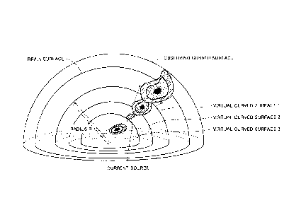
Fig. 2 is a schematic illustration representing a magnetic field generated by
a
current source, observed on an appropriate curved surface.
As can be seen from Fig. 2, when a virtual surface is prepared between an
observing surface and the current source, it is possible to recover the
electromagnetic
field formed by the current source on the observing surface by causing an
appropriate
flow of current on the virtual surface, in accordance with the "principle of
electromagnetic field recovery."
Fig. 3 is a schematic illustration representing a relation between a current
source
in the brain and a plurality of virtual curved surfaces.
Referring to Fig. 3, considering that the electromagnetic field formed by the
current attenuates in inverse proportion to the square of distance, the
expansion of
current on the virtual curved surface (virtual curved surface 2) equivalent to
the current
source becomes wider as the virtual surface is further away from the current
source.
Therefore, the expansion of the current on virtual curved surface 1 is wider
than that on
virtual curved surface 2.
On a virtual curved surface (virtual curved surface 3) on the side opposite to
the
observing surface with respect to the current source, it is impossible to
fully recover the
electromagnetic field formed on the observing surface by the current source.
According to the present invention, based on the principle described above,
the
current source is estimated from the observed data of the electromagnetic
field on the
observing surface.
(Principle of current source estimation)
Assume that a magnetic field (or an electric field) formed by a current source
generated in the brain is observed on an observing surface that is close to
the surface of
the brain, as shown in Fig. 2.
- 14 -
CA 02471746 2004-06-25
A virtual curved surface in the brain is considered, and current distribution
on
the virtual curved surface that recovers the observed magnetic field is
calculated.
When the virtual curved surface is moved to the inner side of the brain with
the radius
made gradually smaller, the expansion of the current distribution recovering
the
observed magnetic becomes smaller, and it becomes the smallest when the
virtual
surface encompasses the true current source. When the virtual curved surface
is
further moved to be deeper than the current source, the expansion of current
distribution
comes to be wider again, and the difference between the magnetic field
generated by the
current and the observed magnetic field also becomes larger.
Accordingly, the depth of the current source can be identified by reviewing
the
expansion of the current distribution recovering the observed magnetic field
and the
error in recovery of the magnetic field. Further, by calculating the current
distribution
on the virtual curved surface at the depth identified in this manner, the
expansion of the
current source can also be found. The foregoing is the principle of the
present
invention.
(Identification of current source depth by Bayesian estimation)
In order to specifically implement the principle of current source estimation
described above, in the present invention, a procedure based on the following
probability
theory is employed. The procedure will be summarized in the following.
What can be observed by MEG or EEG is several to several hundreds of
magnetic fields (electric fields) existing near the surface of the brain. In
order to
approximate the current distribution on the virtual curved surface, lattice
points are set
on the virtual curved surface, and a current dipole (or an appropriate current
source
model) is allocated to each lattice point. In order to estimate the current
distribution
2 5 with high resolution, it is necessary to increase the number of lattice
points to increase
the density of the lattice points.
When the number of lattice points on the virtual curved surface is increased
to be
larger than the number of observation points, a unique solution cannot be
determined.
- 15 -
CA 02471746 2004-06-25
When estimation points is larger in number than the observation points, the
number of
parameters to be estimated becomes larger than the number of observed data,
and hence,
the observed magnetic field would be better recovered even on a virtual
surface that is
positioned deeper than the current source.
In order to cope with such problems, the current distribution on the virtual
curved surface is estimated utilizing Bayesian estimation theory. At the time
of
Bayesian estimation, prior distribution that represents prior information of
the current
source is used. Specifically, as it is considered that brain current sources
exist localized
at a plurality of positions, a prior distribution that leads to the smallest
possible
expansion of current distribution is introduced. Namely, a prior distribution
is
introduced in which a current dipole on a lattice point of which magnitude
cannot be
well identified only from the observed data comes to have a magnitude close to
zero.
This can be realized by introducing hierarchical prior distribution referred
to as
"Automatic Relevance Determination" prior distribution (Reference: R. M. Neal,
Bayesian Learning for Neural Networks, Springer Verlag, 1996). This prior
distribution will be hereinafter referred to as "localized condition prior
distribution."
The manner how to select a prior distribution introducing prior information
other than
the localized condition will be described later with reference to the second
embodiment.
It is impossible, however, to analytically calculate posterior probability
distribution from the localized condition prior distribution and observed
data.
Therefore, in the present invention, variational Bayes method is used as will
be described
later (Reference: H. Attias, Proc. 15th Conference on Uncertainty in
Artificial
Intelligence pp. 21-30, 1999 and Masa-aki Sato, Neural Computation, 13, 1649-
1681,
2001). It is noted that other method of approximation such as Monte Carlo
method
may be used.
By Bayesian estimation using localized condition prior distribution, it
becomes
possible to obtain a current distribution on the virtual curved surface that
recovers the
observed data and has smallest possible expansion. Further, by comparing model
- 16 -
CA 02471746 2004-06-25
posterior probabilities when estimations are made using virtual curved
surfaces of
different depths, the depth of the current source can be estimated.
The logarithm of the model posterior probability can be represented as a sum
of
log-likelihood term and model complexity term. The log-likelihood term becomes
larger as recovery error becomes smaller.
The model complexity term becomes larger when the number of effective current
dipoles (that is, having a magnitude not smaller than an appropriate
threshold) on the
lattice points becomes smaller. As already described, the recovery error and
the
expansion of the current distribution on the virtual curved surface (number of
effective
current dipoles) become the smallest when the depth of the virtual curved
surface
matches the current source. Thus, it can be understood that the model
posterior
probability becomes the largest at this time. In other words, the current
source exists
on the virtual curved surface at a depth at which the model posterior
probability
becomes the largest.
In summary, the present invention provides a method of estimating the position
of the brain current source, depth direction inclusive, from the observed data
of MEG
and EEG.
The basic idea of the present invention comes from the fact that an
electromagnetic field generated by a current source can be recovered by
causing an
appropriate current flow over a curved surface existing between the current
source and
an observing surface, and that the expansion of current distribution on the
curved
surface becomes smaller as the curved surface comes closer to the current
source, as
described above. The present invention is characterized in that, base on this
idea, the
position of the current source including the depth direction is estimated by
considering
the fact that the model posterior probability becomes the largest when the
curved
surface encompasses the current source in Bayesian estimation of the current
distribution on the curved surface that recovers the observed data, that is,
by considering
the model posterior probability.
- 17
CA 02471746 2004-06-25
(Where there are plurality of current sources)
Though description has been made on one current source, the method is also
applicable even when there are a plurality of current sources.
The electromagnetic field generated by a current attenuates in inverse
proportion
to the square of distance, and therefore, the current source closest to the
brain surface
has the largest influence on the observed magnetic field on the brain surface.
Therefore,
it is possible to identify the current sources one by one in order, starting
from the one
closest to the brain surface.
When the virtual curved surface is moved deeper from the brain surface, the
model posterior probability attains the relative maximum near a current source
closest to
the brain surface (which will be referred to as the first current source).
When there are
two or more current sources, there will be a plurality of local sets of
current dipoles
corresponding in number to the current sources, in the current distribution on
the virtual
curved surface.
The local set of current dipoles is referred to as localized current
distribution.
A local surface including individual localized current distribution is
separated and moved
in the depth direction to find the model posterior probability. When the local
surface
that corresponds to the first current source is moved, the model posterior
probability
attains to the relative maximum at the depth of the first current source. When
other
local surfaces are moved, the model posterior probability never attains to the
relative
maximum at the depth of the first current. Thus, the position of the first
current source,
that is, the position of the current source closest to the brain surface can
be identified.
In order to find the second deepest current source, the local surface
corresponding to the first current source is fixed, the depth of the remaining
local
surfaces are aligned and gradually made deeper. Then the model posterior
probability
attains the relative maximum at the second deepest current source. When the
individual local surface is moved in the depth direction again, the model
posterior
probability attains to the relative maximum at the depth of the second current
source,
- 18 -
CA 02471746 2004-06-25
only when the local surface corresponding to the second current source is
moved. In
this manner, the position of the second current source can be identified. The
third and
the following current sources can also be identified in the similar manner.
The method is advantageous over the method in which the depth of individual
local surface is moved independently, in that the time for computation can
significantly
be reduced.
(Method in which resolution is increased gradually)
According to the method of estimating brain current source of the present
invention, it is possible to identify position of each of the current sources
starting from
the one closest to the brain surface in the above described manner and, in
addition, it is
possible to gradually increase the resolution of current source estimation.
First, a position of a current source is roughly estimated with a low
resolution
(with a small number of lattice points on the virtual curved surface and a
small number
of sample points in the depth direction). In this stage, the position of a
local surface
corresponding to each current source is approximately determined.
Next, estimation is made with higher resolution. At this time, the area of the
local surface has become smaller as compared with the original virtual curved
surface,
and hence the resolution is naturally higher when the same number of lattice
points are
used. Accuracy in estimating the current source position can be improved by
increasing the resolution in the depth direction as well. If the current
distribution is
further localized when the resolution is made higher, it is possible to
estimate again with
local surface made smaller and the resolution made still higher.
On the contrary, if the expansion of current distribution does not much vary
even
when the resolution is improved, it means that the current source expands
wide. In this
manner, the resolution can be adjusted in accordance with how the current
source
expands.
[Specific procedure of current source estimation]
In the following, specific procedure for identifying the position of a "brain
- 19
CA 02471746 2004-06-25
current source" will be described in detail, in accordance with the outline
above.
[(I) Preparation for current source estimation]
First, preparation for the process procedure for estimating the current source
will
be described.
Specifically, for the estimation of current source, the following procedures
must
be taken in advance.
(I-1) Determination of the shape of virtual curved surface and current model
(I-2) Further, in order to estimate the virtual current distribution while
moving
the virtual curved surface, it is necessary to determine sample points on the
virtual
curved surface and sample points in the depth direction.
(I-3) Further, as will be described in detail later, it is necessary to
determine in
advance meta parameters to designate the distribution shape of hierarchical
prior
distribution for estimating current distribution as initial values.
In the following, the procedure of (I-1) Determination of the shape of virtual
curved surface and current model will be described in grater detail
(I-1-1) Determination of the shape of virtual curved surface
The simplest shape of the virtual curved surface is obtained by regarding the
brain as a hemisphere and assuming various hemispheres of different radii to
be the
virtual curved surfaces.
When a location where existence of a brain current is highly likely such as
the
cerebral cortex has been known in advance by other measuring method such as
Magnetic Resonance Imaging: MRI, the shape of the virtual curved surface may
be
determined based on such information.
Particularly when the shape of the cerebral cortex is known with high
precision
and it is considered that the brain current source is non-existent in other
regions, the
current distribution estimation of cerebral cortex points may be performed
while
omitting the search in the depth direction, which will be described later.
Further, it is
also possible to perform the search in the depth direction only in a limited
region.
- 20
CA 02471746 2004-06-25
In this case, the shapes of virtual curved surfaces having different depths
may
generally differ. It is necessary, however, to determine the shapes not to
intersect with
each other.
(I-1-2) Determination of current model
As a current model on the virtual curved surface, let us consider a current
dipole
model. It is also possible to consider other current models.
Consider appropriate lattice points (sample points) {Xõ1n=1,..., N} on the
virtual
curved surface. Assume a current dipole of which current intensity is jn on
each lattice
point. Here, the magnetic field formed by the current dipole jn at a lattice
point Xn on
an observation point Yi (i=1, ..., I) on the brain surface is given by the
following Biot-
Savart's expression.
jn x (Y; ¨ Xn)
Y, ¨ Xn13
Here, u represents magnetic permeability, and by way of example, for a vector
Xn, the expression1Xnlrepresents the absolute value of vector Xn. As more
accurate
expression, Sarvas's expression with the brain regarded as a sphere filled
with
conductive solution (Reference: J. Sarvas, Phys. Med. Biol. 32, 11-22, 1987)
may be
used, or numerical solution such as given by finite element method or boundary
element
method may be used, considering detailed structure of the brain. In the
following,
Biot-Savart's expression above will be used, for simplicity of description and
representation.
Here, the magnetic field formed by the current dipole {in 1n1, N} on an
observation point Yi (i=1, ..., I) is represented by the following equation.
N X (Y, ¨X.)
n=1 1Y; ¨ Xn13
- 21
CA 02471746 2004-06-25
Assuming that the direction of the magnetic field observed at the observation
point Yi is a vector Si,n (c=1, C), component Bi,n in the direction of
vector Si,n of the
magnetic field at this point can be given as
õN ( in X (.17, ¨ X.))=
=
n=1 Yj ¨3(.13
Further, when a local gradient of a magnetic field is to be measured as a
magnetic field to be observed, a differentiation of the equation above by Yi
will be
observed.
When the direction of a current dipole at a lattice point Xn (position vector)
is
restricted, the current dipole can be represented by the following equation,
with a
possible independent direction of the current dipole being bn,d(d=1, D). In
this
equation, a case where D = 3 corresponds to a case where there is no
restriction on the
direction.
in =bn,d
d=1
In summary, a magnetic field formed by the current dipole at a lattice point
{Xn
ln=1, N} of the virtual curved surface on the observation point Yi can be
given as
N D
= Eiõ, = G(i,c; n,d)
n=1 d=1
(bn d x (Yi Xn))=
G(i,c; n,d ) = ______ '
3
X.
- 22
CA 02471746 2004-06-25
Here, jõ,d is an independent component of the current dipole at the lattice
point
Xn. Further, the function G (i, c; n, d) represents the component in
Si,n direction of the
magnetic field formed by the current dipole jn,d at the lattice point XII.
The problem of estimating current distribution may be considered as a problem
of estimating a current distribution on the virtual curved surface {jn,d I
n=1, N;
d=1, D} from the observed magnetic field {Bi,n Ii=1, c=1, C}.
The measured value of the magnetic field at the observation point described
above may be given by the following matrix expression. Here, G is referred to
as a
lead field matrix. When Sarvas's expression or a numerical solution such as
obtained
by the boundary element method is used in place of Biot-Savart' s expression,
the lead
field matrix will have different values, and other portions of the following
description are
similarly applicable.
B = G = J
B=(B i = 1, = = =, I; c = 1, = = =, C) : (I x C) dimensional vector
Jn,dl n =1,= ==,N; d = 1,= = =, D) : (N x D) dimensional vector
G = (G(i,c;n,d) I i =,I; c = 1,= = =,C;
n = 1,= = =,N; d = 1,= = =,D)
: (I x C) x (N x D) dimensional matrix
(Current source probability model)
With the current model determined in this manner, the following "current
source
probability model" is introduced for such current distribution estimation.
(1-1-3) Current source probability model
A probability model for the current model on the virtual curved surface
described above will be considered.
It is assumed that the observed magnetic field is represented as a sum of the
- 23 -
CA 02471746 2004-06-25
magnetic field formed by the current distribution J on the virtual curved
surface and the
observation noise. Further, it is assumed that the observation noise is
Gaussian noise
having an independent variance a2 at each measuring point.
More generally, it may be possible to consider Gaussian noise having a multi-
dimensional normal distribution, in which correlation between noises at
respective
measuring points is represented in the form of a covariance matrix. For
simplicity of
description, an isotropic homoscedastic noise model will be employed in the
following.
Specifically, the observed magnetic field is considered as
B = G= J +
= .1 virtual curved surface= in,d = 1, = = =,N; d =1,= = = , D)
G = (G(i,c;n,d) I i =1,= = =, I; c = 1,= = =,C; n = 1,= = =,N; d = 1,...,D)
= = 1,= = =J; = 1,= = =,c)
: Gaussian noise with each component having independent variance a2
The probability distribution for the current model may be considered as
follows.
First, a virtual surface at a specific depth, or a set of local surfaces with
the depth
of each local surface identified, will be represented by M. When a current
distribution J
on the virtual curved surface M is given, the probability P (B I J, p, M) that
the
observed magnetic field is B is represented by the following equation, where
p= 1/a2.
P(B I J,13,M) = exp[--113IB ¨ G= JI2 +-1 C)log(f3/27c)]
2 2
J3 = 1 / a2
(1-1-4) Hierarchical prior distribution
As already described, localized condition hierarchical prior distribution will
be
- 24
CA 02471746 2004-06-25
used as the prior distribution for the current distribution J on the virtual
curved surface
M.
The prior distribution for the current distribution J before observation
(probability of J being realized) is represented by the following equation,
under the
assumption of localized condition hierarchical prior distribution.
1 N
la,13,M)= exp[---pIan(Ein,d)2
¨D log (Plan / 27c
2 n=1 d=1 2 n=1
P0(131TX) = r(1311/T)Y130)
Here, F (...) represents gamma distribution, which is defined below. In the
expression below, r (yo) is a gamma function, which is also defined below.
1
r(01b,70)---0,00/b)" ______ 1 e-yeab
F(y0)
r(yo) f dt t"-1
0
Further, a and T are hyper parameters introduced to model the current
distribution J and prior distribution for inverse variance of noise p.
Hierarchical prior
distributions Po (a M) and Po (TIM) for a and T are
P0(a1M) = fir(anlao,Ycco)
n=1
PO (r IM) F(T Yto)
- 25
CA 02471746 2004-06-25
In the equations above, meta parameters bar ao, 'No, To and bar yto
determining
the distribution shape of the hierarchical prior distributions Po (alM) and Po
(TIM) for
ccand T will be described in detail later. Here, "bar" preceding a name of a
variable
means that the variable has the sign "¨" thereabove.
(I-1-5) Bayesian estimation
When data B of a magnetic field is observed, the posterior probability
distribution P (JIB, M) that the current distribution is J can be calculated
in the following
manner, using Bayesian theorem.
P(JM, M) = Jd13 da dT P (J, a, T IB, M)
Here, the posterior probability distribution P (J, 0, a, TIB, M) is given as
P(J, P,a,T IB,M) =
P(B IJ,13,m)P0(.1 la, I3,M)P0(13 IT,M)P0(a1M)P0ec IM)
P(BIM)
P(B IM) =
dJdfliclocdT P ( B I J,13, M)P0(J m) Po (3 I m) Po (a Im)P0 (T IM)
Using this posterior probability distribution, an expected value E[JIB, M] is
given
as
J = E[J IB,M] = f dJdfidadz-P (J, AMP
- 26
CA 02471746 2004-06-25
Further, P (BIM) represents marginal likelihood of the virtual curved surface
model M. When the depth of a current source is estimated, a number of models
having
different depths are compared. At this time, it is assumed that there is no
prior
information about the depth. Specifically, in the following, it is assumed
that P(M) =
constant.
When the observation data B is given, the probability that the model M is a
true
model, that is, the model posterior probability P(MIB), is in proportion to
the model
marginal likelihood P(BIM) under the assumption described above, and hence,
the
following relation holds.
P(MIB) cc P (B IM)
(1-1-6) Variational Bayes method
It is generally impossible to analytically calculate the model marginal
likelihood
when the probability model and the hierarchical prior distribution are given.
Therefore, as a method of calculating by approximation the model marginal
likelihood, variational Bayes method is used. It is possible to use other
method of
approximation, such as Monte Carlo method and Laplacian approximation.
The "variational Bayes method" will be briefly outlined, and specific
procedure
will be described later.
In order to calculate a true posterior distribution P (J, 0, a, TIB, M) by
approximation, a trial posterior distribution Q(J, 13, a, t) is considered.
Closeness between the two probability distributions P (J, 0, a, TIB, M) and
Q(J,
0, a, -c) can be calculated by using K-L distance given by the following
expressions.
KL(Q P)
.1,
= f dJd0dadtQ(J, (3, a, t)log[ Q(,13,at)
P,a,t l B,M)
- 27
CA 02471746 2004-06-25
= logP(B IM)¨ F(Q) 0
F(Q) f dJdr3dccdt Q ( J, 13, a, -c ) x
log[P(B 1.11,13,M)P0(.1 la, 13,M)P0 (I3 IT,M)Po (a IM)P0 (t IM)
Q(J,(3,a,T)
The K-L distance attains to zero only when the two distributions are equal to
each other, and otherwise it always assumes a positive value.
When a free energy F(Q) for the trial posterior distribution Q is defined in
the
expression above, the following inequality results.
F(Q) logP(B IM)
Specifically, the distribution Q(J, f3, a, -c) that maximizes the free energy
F(Q)
becomes equal to the true posterior distribution P (J, p, a, TIB, M), and at
this time, the
free energy is equal to the marginal log-likelihood.
According to variational Bayes method, the form of function Q(J, p, a, t) is
restricted to the following form, to maximize the free energy.
Q(.1", 13,11,T)= QJ(J,13)Qc,(a,c)
By alternately repeating the step of fixing the second term Qa on the right
side
of the equation above and maximizing F(Q) with respect to the first term Qj on
the right
side and the step of fixing the first term QJ and maximizing F(Q) with respect
to the
second term Qa, a distribution Q* is obtained that attains the relative
maximum of free
energy F(Q).
[(II) Procedure of current source estimation]
A specific procedure for estimating the current source after the preparation
- 28
CA 02471746 2004-06-25
above will be described with reference to the figures.
Fig. 4 is a flow chart representing an overall procedure of the brain current
source estimating method in accordance with the present invention.
Referring to Fig. 4, first, when the process of estimating a position of a
brain
current source starts (step S100), values of meta parameters for designating
the shape of
hierarchical prior distribution for estimating the current distribution and an
initial value
of a variable to be estimated are determined (step S102).
Thereafter, initial estimation of the current source is performed, using an
initial
resolution, so as to extract candidates of the current source (step S104).
Then, among the current source candidates extracted in this manner, a position
of a current source that is closest to the brain surface is estimated (step
S106).
Thereafter, depths of other current sources is identified successively (step
S108).
After the positions of current sources are identified with the first
resolution in
the above described manner, re-estimation of the positions of the current
sources is
performed with the spatial resolution increased (step S110), and the process
ends (step
S112).
Processes of respective steps of Fig. 4 will be described in grater detail in
the
following.
(II-1) Initial estimation of current source using initial resolution
(extraction of
current source candidates)
Fig. 5 is a flow chart representing the process of step S104 among the steps
shown in Fig. 4, that is, the process of initial estimation of the current
source using an
initial resolution.
Referring to Fig. 5, first, sample points in the depth direction with the
initial
resolution are determined to be {Rkik=1, K} . Current
distribution is estimated for
the virtual curved surface at each depth Rk. Further, based on the current
distribution
estimated in this manner, posterior probability for each depth Rk is
calculated. The
posterior probability corresponds to the free energy value, which will be
described later
- 29
CA 02471746 2004-06-25
(step S202).
For the current distribution at the depth Rm at which the posterior
probability
calculated in this manner becomes the highest, a relative maximum point of
current
intensity is found (step S204).
Further, a local surface that encompasses each relative maximum point is
determined. Assuming that there are L local surfaces, each local surface will
be the
candidate of localized current source (step S206).
In the following, the process of step S102 of Fig.4 and the process of step
S202
of Fig.5 that follows, will be described in grater detail.
(II-1-1) Determination of meta parameter values for designating shape of
hierarchical prior distribution for estimating current distribution and
initial values of
variables to be estimated
As described above, estimation of a current source is performed using
variational
Bayes method. Therefore, the process of step S102 shown in Fig. 4 is performed
in the
following manner, with the application of variational Bayes method.
By way of example, the meta parameters designating the shape of hierarchical
prior distribution are determined as follows.
Yoo =1 (more generally, 0 ypo)
= 0 (more generally, 0 y.,0)
yao = 0.1 (more generally, 0 yao)
= = Vie (13)) KT = 1 (more generally, I(T1)
1 I C
I =C ,.1 ..1
- 30 -
_
_
CA 02471746 2004-06-25
I c
T3- = ______________ EBi
I=C 1.1 c=1
= Ka, = ¨1 Tr (G' = G), K = 10 (more generally, 0 < Ka)
N = D = N
Further, based on the equations above, each variable is initialized in the
following manner.
yi3 = 1 ¨2I = C +
YT = Yto Ypo
1
Y =y
7d. =
=
EG = G' = G
(II-1-2) Specific process of variational Bayes method for estimating current
distribution
(1) Calculation of expected values of parameters J, J3 (J-step process)
Here, expected values of parameters J and 13 are calculated. By this process,
the free energy F(Q) for Qj is maximized.
By defining a diagonal matrix A as follows, QJ is derived in accordance with
the
following equations. In the following equations, an expected value of a
variable is
- 31
_
CA 02471746 2004-06-25
represented by the variable name with "¨" attached thereabove.
A(n, d; n', d') = 8,õ,,Sdd,Un (n, n' =1,= = =,N; d,d' =1,= = =,D)
E = EG +A.-
= E-i
13 =yi[-I-dB-G.112 +1JA-1+yp0ti]-1
2 2
QJ(J,13)=QJ(J10)Qp(13)
1 1
%PIO) = exp[--13(J-TIE(J-T)+-loglE1+-1IC-Ilog(13/2rc)]
2 2 2
Qp (0) = r(13 Yp)
(2) Calculation of expected values of hyper parameters, that is, calculation
of
expected values of parameters a, -c (process for a-step)
Following the J step, expected values of hyper parameters cc and T are
calculated.
In this step, a process is performed to maximize the free energy F(Q) for Q.
The procedure can be represented as
D D
= y[ y' +--j.2 d +E(E-1)(n, d ; n, d )]-1 (n = 1, = = = , N)
2 d=1 d=1
7C.
= [y' +YpX]-'
Qc,(a,t) = F(r y,)nr(an Idn,Ycc)
n=1
(3) Calculation of free energy
- 32
CA 02471746 2004-06-25
Using QJ and Qa. calculated through the J step and a step as described above,
the
free energy is calculated in the following manner.
F=LP+H3+1-10+Ha+H,
1
LP = ¨ ¨ G = j ¨ Tr E-1EG + ¨21 (1 = C)
(< log[3 > ¨ log 27r)
2 2
< logr3 >. log [3 + (yo) ¨ log yo
d ( log F(y))
NJ(Y) w: digamma function
dy
1 ¨ ¨
H, = ¨ ¨ [Tr E-1 i- log E' A ¨ ¨ ¨113 J'Aj
2 2
Ho = yo0[1og(T13-)¨t13-+ 1]+ c13(yroyo0)
(1)(y, yo) (logf(y)¨ yy(y) + y) ¨ (log 1"(y0) ¨ yo logy + Yo)
Yo((Y) ¨ log y)
H. = yto[log(t1tio)¨(t/t0)+1]
= E yao[log can rd,o)¨(d. /Tio) +1]
n=-1
In this manner, the process from the J step to calculation of free energy
described above is repeated until the value of free energy F converges. The
value of
free energy F(Q) after convergence gives an approximation of marginal log-
likelihood
log P (BIM).
Further, model log-posterior probability differs only by the constant from log
P
(BIM), and therefore, the model having the maximum model posterior probability
is the
same as the model of which free energy is the highest, in accordance with the
above
described approximation.
- 33
CA 02471746 2004-06-25
By the above described procedure, posterior probability for the depth Rk can
be
calculated. By performing the processes of steps S204 and S206 of Fig. 5
accordingly,
it is possible to find candidates of current sources localized to respective
local surfaces.
(II-2) Identification of current source closest to the brain surface
Next, the process of step S106 of Fig. 4, that is, the process for identifying
the
current source closest to the brain surface among the candidates of current
sources
found in the manner as described above, will be described.
Fig. 6 is a flow chart representing a process for identifying a current source
closest to the brain surface.
First, as the initial value, the value of a variable 1 is set to 1 (step
S302). Then,
the variable 1 is compared with a possible maximum value L of variable 1 (step
S304),
and when the variable 1 is not larger than the maximum value L, the process
proceeds to
step S306, and when the variable 1 exceeds the maximum value L, the process
proceeds
to step S324 (step S304). Specifically, the process from step S306 to step
S322 is
repeated from 1=1 to 1=L.
In step S306, depth of a local surface other than the lth local surface is
fixed at
the depth Rm calculated in step S204 of Fig 5.
The value of variable k is set to 1 (step S310). Thereafter, the variable k is
compared with a possible maximum value K of variable k (step S310), and when
the
variable k is not larger than the maximum value K, the process proceeds to
step S312,
and when the variable k exceeds the maximum value K, the process proceeds to
step
S320.
In step S312, the depth of the lth local surface is first determined to be Rk.
Thereafter, current distribution is estimated for the set of L local surfaces
(step
S314).
Thereafter, the posterior probability (free energy) for this arrangement of
the
local surfaces is calculated (step S316). By incrementing the value of
variable k by
only 1 (step S318), the process returns to step S310.
- 34
CA 02471746 2004-06-25
The process is performed for each of the local surfaces having the depths from
k=1 to k=K, and then, the depth Rm(1) of the first local surface that provides
the highest
posterior probability is calculated (step S320). By incrementing the value of
variable 1
only by 1 (step S322), the process returns to step S304.
In this manner, among the depths Rm(1) calculated for each variable 1, one
closest
to the brain surface (shallow) is detected, which is denoted by 11 (step
S324).
Through the steps described above, it follows that the lith local surface
corresponds to the current source closest to the brain surface, the initial
estimate value
of the depth thereof is calculated as Rm(li), and the process terminates (step
S326).
(II-3) Identification of depth of current source corresponding to each local
surface
Figs. 7 and 8 are flow charts representing a process for identifying depth of
a
current source corresponding to each local surface.
Referring to Fig. 7, the value of a variable s is set to 1 as an initial value
(step
S402). Thereafter, the variable s is compared with a possible maximum value L
of
variable s (step S404), and when the variable s is not larger than the maximum
value L,
the process proceeds to step S406, and when the variable s exceeds the maximum
value
L, the process proceeds to step S434 (step S404). Specifically, the process
from step
S406 to step S432 is repeated from s=1 to s=L.
In step S406, when the depths of local surfaces identified so far are
represented
as {Rm(11), Rm(18)}, the depths of these local surfaces are fixed at
{Rm(11), R(1)),
respectively (step S406).
First, it is assumed that 1 is not equal to any of {11,..., 1.}, and that I
belongs to a
set of {1, ..., L} (step S408). Then, whether all possible values are
considered as the
value of variable 1 or not is determined (step S410), and if all the possible
values have
been considered, the process proceeds to step S430. Otherwise, the process
proceeds
to step S412.
In step S412, the depth of a local surface that is different from the Ith
local
- 35
CA 02471746 2004-06-25
surface and not any of L} is fixed at Rm.
The value of variable k is set to 1 (step S414). Thereafter, the variable k is
compared with a possible maximum value K of variable k (step S416), and when
the
variable k is not larger than the maximum value K, the process proceeds to
step S418,
and when the variable k exceeds the maximum value K, the process proceeds to
step
S426. Specifically, the process from step S418 to step S424 is repeated from
k=1 to
k=K.
In step S418, the depth of the first local surface is set to Rk..
Thereafter, for the set of L local surfaces, current distribution is estimated
(step
s420).
Further, posterior probability (free energy) for this arrangement of the local
surfaces is calculated (step 422).
Referring to Fig. 8, in step S426, after the process to k=K is finished in the
above described manner, the depth Rm(1) of the lth local surface attaining the
highest
posterior probability is calculated (step S426).
Then, other variable 1 that is not equal to any of {li, ..., 1.} belongs to
the set of
{1, ..., L} and is not yet processed is selected (step S428), and the process
returns to
step S410.
Through the above described steps, among Rm (1) values corresponding to all
the
processed variables 1, the value 1 that is closest to the brain surface is
calculated and
denoted by 1 s+1 (step S430).
Further, s is replaced by s+1 (step S432), and the process returns to step
S404.
When the process ends for all the possible values s, identification of the
depths of
current sources corresponding to respective local surfaces is finished (step
S434).
(II-4) Re-estimation with increased resolution
Figs. 9 and 10 are flow charts representing the process of step S110 shown in
Fig. 4, that is, the process for re-estimating a position of a current source
with higher
spatial resolution.
- 36 -
CA 02471746 2004-06-25
Referring to Figs. 9 and 10, first, numbers of local surfaces corresponding to
the
current sources estimated using the initial resolution are re-numbered so that
the
surfaces have the numbers 1, 2, 3, ..., L starting from the one closest to the
brain surface
(step S502). Then, corresponding to the expansion of current distribution on
each
local surface, the local surface is made smaller (step S504).
The depth of the local surface Rm(1) calculated by the process up to step S108
of
Fig. 4 is denoted as Rm'id(1) (step S506).
New resolution and search width in the depth direction are respectively
represented as AR and (KL, = AR). Further, resolution of lattice points on the
local
surface is also increased (step S508).
The value of a variable 1 is set to 1 as an initial value (step S510).
Thereafter,
the variable 1 is compared with a possible maximum value L of variable I (step
S512),
and when the variable 1 is not larger than the maximum value L, the process
proceeds to
step S514, and when the variable 1 exceeds the maximum value L, the process
proceeds
to step S534 (step S512). Specifically, the process from step S514 to step
S532 is
repeated from 1=1 to 1=L.
In step S514, the depth of a local surface l' other than the lth local surface
is
fixed to Rm'id (1').
Further, the process from step S518 to step S526 is performed with k=0, 1,
- KL.
First, the value of variable k is set to 0 (step S516). Thereafter, the
absolute
value of variable k is compared with the possible maximum absolute value Of KL
(step
S518), and when the absolute value of variable k is not larger than the
maximum value
KL, the process proceeds to step S520, and when the absolute value of variable
k
exceeds the maximum value KL, the process proceeds to step S528 (step S518).
In step S520, the depth of the lth local surface is set to (Rm0id(1)+k = AR).
Thereafter, for the set of L local surfaces, current distribution is estimated
using
the present resolution (step S522).
- 37
CA 02471746 2004-06-25
Further, posterior probability (free energy) for this arrangement of the local
surfaces is calculated (step S524). Then, the value k is set to the next one
of { 1,
- 1(0, and the process returns to step S518.
After the above described process is performed until k= 1(L, the value k that
provides the highest posterior probability is calculated in step S528, which
value is
denoted by km.
Then, Rm01d(1) is replaced by Rm'Id(1)+km = AR (step S530) The value of
variable 1 is incremented by only 1 (step S532), and the process returns to
step S512.
When the above described process has been performed until the value of
variable
I attains to the maximum value L and the resolution has reached the final
resolution (step
S534), the process is terminated (step S538).
When the resolution is not yet the final resolution (step S534), the
resolution of
the lattice points on the local surface and the resolution in the depth
direction are
increased (step S536), and the process returns to step S510.
By the "method of estimating brain current source" as described above, it
becomes possible to estimate the position of a brain current source, including
the
position in the depth direction, from observation data of MEG (or EEG).
Further,
such estimation in the depth direction is applicable even when there are a
plurality of
current sources. Still further, the method is applicable when the current
sources are
localized as in the case of current dipoles or when the current source has an
expansion.
In addition, by the method, it is possible to estimate how the current source
expands.
By additionally performing the process described with reference to Figs. 9 and
10 after the estimation with the initial resolution, it becomes possible to
successively
increase resolution for estimating a position. This also means that it is
possible to
review with the scope of search restricted based on physiological findings or
data
obtained by other observation method.
[Result of simulation]
In the following, simulation results will be described, in which current
source
- 38
_
CA 02471746 2004-06-25
positions of an assumed model were estimated in accordance with the method of
estimating brain current source described above.
Fig. 11 is a top view of a magnetic field distribution in the radial direction
observed on a surface of a hemisphere, assuming that the human brain is a
hemisphere
having the radius of 10.0 (arbitrary unit).
Fig. 11 shows a magnetic field distribution on a surface of the hemisphere in
which a single current source is positioned at a radius of 7.0 from the
center, as will be
described later. In the simulation that will be discussed below, noise having
the STN
ratio of 0.1 is added to the observation data of the magnetic field.
Fig. 12 represents results of initial estimation of current sources using
initial
resolution.
Fig. 12 shows the result of calculation of current distribution, in which, as
described with reference to the process of steps S102 to S104 of Fig. 4, in
order to
perform initial estimation of the current source using the initial resolution,
the depth
(radius) is changed stepwise and on the hemisphere of each depth, the current
distribution that attains the maximum free energy is calculated in accordance
with
variational Bayes method.
Fig. 12(a) shows the result where the radius is R=5.0, 12(b) shows the result
where the radius is R=6.0 and 12(c) shows the result where the radius is
R=7Ø
Fig. 13 represents results of initial estimation of current sources using
initial
resolution, where the radius is larger (that is, closer to the surface of the
brain).
Fig. 13(d) shows the result where the radius is R=7.5, 13(e) shows the result
where the radius is R=8.0 and 13(f) shows the result where the radius is
R=9Ø
Fig. 14 represents magnitude of free energy on each virtual hemisphere,
obtained
when current distribution that attains maximum free energy is calculated for
virtual
hemispheres at various depths assumed in the brain.
Referring to Fig. 14, it can be understood that the maximum point of free
energy
exists between the radii of 7.0 and 8.0, when calculation is made assuming
that the
- 39
_ _
CA 02471746 2004-06-25
hemisphere as a whole is a virtual curved surface.
As can be seen from Fig. 13(d), one point of relative maximum exists in the
current distribution on the virtual hemispherical surface having the radius of
R=7.5.
As the current source is initially estimated using the initial resolution in
this
manner, on the virtual curved surface having the maximum free energy, a local
surface
that encompasses the relative maximum point of current distribution is
calculated, and
the process for identifying the current source is performed on the local
surface.
Figs. 15 and 16 represent processes for identifying the current source
executed
further on a local surface including a point of relative maximum, with the
resolution of
lattice points on the local surface and the resolution in the depth direction
increased.
Figs. 15(a), 15(b) and 15(c) represent current distribution on local surfaces
where the radius is R=5.0, R=6.0 and R=7.0, respectively. Similarly, Figs.
16(d), 16(e)
and 16(f) represent current distribution on local surfaces where the radius is
R=7.5,
R=8.0 and R=9.0, respectively.
Fig. 17 represents the free energy calculated with the depth of local surface
varied.
Referring to Fig. 17, the free energy as a result of calculation using the
local
surface has the relative maximum value near the radius of R=7, and from the
result, it is
possible to identify that one current source exists at the position of R=7.
The current distribution of the current source at this time is as shown in
Fig.
15(c), and as already described, it can be understood that the current
distribution also
has the narrowest expansion.
Fig. 18 is a top view of a magnetic field distribution observed on a surface
of the
brain assumed as a hemisphere, when there are two current sources in the
brain.
In the example shown in Fig. 18, it is assumed that the current sources are
positioned at the radii of R=6.0 and R=8Ø
Figs. 19 and 20 represent results of initial estimation of current sources
using
initial resolution.
- 40 -
CA 02471746 2004-06-25
Specifically, Figs. 19 and 20 illustrates the process (step S104) for
performing
initial estimation of current sources using the initial resolution shown in
Fig. 4, when
there are two current sources in the brain.
Figs. 19(a), 19(b) and 19(c) represent current distribution on virtual
hemispherical surfaces where the radius is R=5.0, R=6.0 and R=7.0,
respectively.
Figs. 20(d), 20(e) and 20(f) represent current distribution on virtual
hemispherical surfaces where the radius is R=7.5, R=8.0 and R=9.0,
respectively.
Fig. 21 represents radius dependency of free energy, when current distribution
that attains maximum free energy is calculated for each virtual hemispherical
surface of
the whole hemispherical surfaces.
As shown in Fig. 21, when the free energy is calculated over the entire
hemispherical surface, it is understood that the maximum value of free energy
exists
between the radii of R=7 and R=8, that is, near the radius of R=7.5.
As can be seen from Fig. 20(d), on the virtual hemispherical surface having
the
radius of R=7.5, there are two relative maximum points in the current
distribution and
two local surfaces are determined.
Next, the result of calculation corresponding to the process of step S106
shown
in Fig. 4 will be described.
Figs. 22 and 23 illustrates the process for calculating the depth of a lth
local
surface Rm(1) attaining maximum posterior probability, to identify a current
source
closest to the brain surface.
Therefore, Figs. 22 and 23 represent current distribution when a local surface
corresponding to one current source is moved while the other local surface is
fixed on a
surface that attains the maximum free energy calculated over the entire
spherical surface.
Figs. 22(a), 22(b), 22(c) represent current distribution on local surfaces
where
the radius is R=5.0, R=6.0 and R=7.0, respectively.
Figs. 23(d), 23(e) and 23(f) represent current distribution on local surfaces
where the radius is R=7.5, R=8.0 and R=9.0, respectively.
-41
= CA 02471746 2004-06-25
Fig. 24 represents local surface position (radius) dependency of free energy
when a virtual local surface is moved as shown in Figs. 22 and 23.
As shown in Fig. 24, when a local surface corresponding to one current source
is
moved to the position of R=8 while the other local surface is fixed on a
surface that
attains the maximum free energy calculated over the entire spherical surface,
the free
energy is maximized.
Therefore, from the result shown in Fig.24, it can be seen that the position
of the
current source closest to the brain surface is at the radius of R=8Ø
Thereafter, the depth of the other current source is identified.
Here, the depth of the local surface corresponding to one current source is
fixed
at the radius of R=8.0, and the depth of the local surface corresponding to
the other
current source is moved.
Figs. 25 and 26 represent current distribution when one local surface is fixed
on
a specific surface and a local surface corresponding to the other current
source is moved.
Figs. 25(a), 25(b) and 25(c) represent current distribution on local surfaces
where the radius is R=5.0, R=5.5 and R=6Ø
Figs. 26(d), 26(e) and 26(f) represent current distribution on local surfaces
where the radius is R=6.5, R=7.0 and R=7.5.
Fig. 27 represents local surface position (radius) dependency of free energy
when a virtual local surface is moved as shown in Figs. 25 and 26.
As can be seen from Fig. 27, the free energy is maximized at the position of
R=6.
It can be understood that by such a process, even when there are two current
sources in the brain, it is possible to identify the depth of each of the
current sources.
[Second embodiment]
In the following, the second embodiment of the present invention will be
described, in which, among the processes implemented by software (or partially
by
hardware) of the "brain current source estimating method," "brain current
source
estimating program," and "brain current source estimating apparatus" in
accordance
- 42
CA 02471746 2004-06-25
with the first embodiment of the present invention described above, the
processes from
"(I) Preparation for current source estimation" to "(3) Calculation of free
energy" are
modified.
As a background for describing the modifications in accordance with the second
embodiment, the concept of the first embodiment will be summarized in the
following,
and of the basic concept, portions that are modified in the second embodiment
will be
described.
(Concept of virtual curved surface estimation in the first embodiment)
In the first embodiment, as a current model on the virtual curved surface,
current
dipoles on lattice points are assumed, and a process of solving an inverse
problem that
the current distribution J is estimated from observed magnetic field B on the
observation
surface is performed. Here, such an inverse problem is a so called "ill-posed
problem"
and it is difficult to find an exact solution, as (the number of lattice
points at which
current dipoles exist) is generally larger than (the number of observation
points).
In the first embodiment, in order to solve such a problem, the method of
"Bayesian estimation" has been used.
Bayesian estimation utilizes the fact that posterior probability distribution
when
virtual surface M and observed magnetic field B are given can be represented
by the
following equation.
P(JIB,M)=P(BIJ,M)P(JIM)
P(BIM)
Here, P(J1B,M) is the probability distribution on the virtual curved surface M
under the condition that the magnetic field B has been observed, and it
represents the
"posterior probability distribution." P(BIJ, M) is "data likelihood," P(JIM)
is prior
distribution and P(BIM) is marginal likelihood.
The marginal likelihood is given by
- 43
,
CA 02471746 2004-06-25
P(BIM) = ScIJP(BIJ,M)P(J IM)
The posterior probability P(MIB) is given by
P(MIB)=P(BIM)P(M)
cc P(1131M)
P (B)
Assuming that there is no prior information related to the depth, P(M) =
constant, and therefore, the probability that the model M is the true model
when the
observation data B is given is in proportion to the model marginal likelihood
P(M113)
under the assumption above, as already described with reference to the first
embodiment.
Specifically, in the first embodiment, when the current model is selected, a
model
that attains the highest posterior probability, or the highest marginal
likelihood, has been
selected.
For such a process, the marginal log-likelihood log P(BIM) represented by the
following equation is the object of calculation.
logP(BIM)=<log(P(BIJ,M))>, ¨KL(P(JIB,M)1111(JIM))
= (expected log-likelihood) - (distance of prior/posterior distribution)
-(recovery error) - (effective degree of freedom of parameters)
As represented by the equation above, that the marginal log-likelihood is
maximized corresponds to a concept that the error and the effective degree of
freedom
of parameters are minimized, in other words, that the error and the expansion
of current
distribution are minimized.
In the first embodiment, the problem of maximizing the marginal log-likelihood
- 44 -
CA 02471746 2004-06-25
described above has been solved by the so called "variational Bayes method" in
which
the trial posterior distribution Q is introduced as an approximation of the
posterior
distribution, and the posterior distribution is determined to maximize the
free energy (Q).
(Concept of prior distribution in the first embodiment)
In the first embodiment, as a prior information of the brain current source, a
localized condition that the current sources exist at a plurality of positions
in the brain is
used, which is represented in the form of hierarchical prior distribution.
Specifically,
hyper parameters an (n=1, N) are introduced and the form of the
hierarchical prior
distribution given by the following expressions are assumed.
1 N
Po ( J la,13) cc exp [¨ ¨PEanl µ1,112]
2 n=i
Po (an Rio Yco ) cc exp [ ¨ Y.0 an hao (Yao ¨1)10g an]
From the expressions above, it can be understood that the hyper parameter an
is
in proportion to inverse variance (the reciprocal of variance) of current L.
When the
values of variance of current In and inverse variance p of noise are known in
advance, a
prior distribution may be used in which the value a. is fixed to the value
calculated from
the values of variance of current and inverse variance of noise. The value of
variance
of the current, however, is generally unknown, and therefore, in the first
embodiment, a
hierarchical prior distribution Po (cc.lbar cco yao) for the hyper parameter
ofõ is assumed,
and Bayesian estimation is performed on an.
Here, bar an and 'No are meta parameters for determining the shape of
hierarchical prior distribution, and common values are assumed for every an.
When
Bayesian estimation is performed using the localized condition hierarchical
prior
distribution, Bayesian estimation that recovers the observed data with
smallest possible
number of current dipoles is performed as described above.
- 45 -
--
CA 02471746 2004-06-25
Minimum norm estimation method, which is often used in current source
estimation of MEG (Reference: M. S. Hamalainen and R. J. Ilmoniem, Med. &
Biol.
Eng. & Comput., 32, 35-42, 1994) corresponds, from the view point of Bayesian
estimation, to a process in which the value an as the prior distribution is
made common
to all the points, and the value is directly determined to be an appropriate
value.
In the minimum norm estimation, total sum of current intensities at all the
points
is to be minimized, and hence points having small current intensities appear
in large
number in the estimated solution. Therefore, this method is disadvantageous in
that it
is difficult to determine whether such small current distributions represent
the true
current distribution or noise derived from estimation error.
The localized condition hierarchical prior distribution solves this problem of
the
minimum norm estimation method.
(Modifications in the second embodiment)
In the second embodiment, prior distribution considering not only the local
condition but also continuous condition is assumed. When current source
distribution
is to be estimated with high precision with the spatial resolution in the
order of
millimeters, it is necessary to consider continuity of current distribution.
Actually,
neural cells in the cerebral cortex has a columnar structure having the radius
of about 10
mm, and when a neural activity takes place, it is likely that neural cells in
an area having
the radius of about 20 mm fire simultaneously. Considering such points, in the
second
embodiment, a hierarchical prior distribution is assumed that combines the
local
condition and continuous condition, as will be described in the following.
In order to introduce the continuous condition, an internal variable Z is
newly
introduced, and the current J is represented as the internal variable Z
smoothed through
a smoothing filter W. Here, though not limiting, a Gauss filter may be used as
such a
smoothing filter W. Now, the prior distribution can be represented as
- 46
CA 02471746 2004-06-25
1 N
Po (J IZ,c03) oc exp [¨ ¨43Ian(J. ¨ W = Zõ)2]
2 n=1
1 N
Po (Z I 21.) OC exp [¨ ¨I3E kn I Z.121
2 n=1
In the prior distribution above, integration of Z can be executed easily, as
represented by
Po(Jia,P,X)=IdzPo(JIz,a,p)Pocz
oc exp =A-1=W')-1.J]
2
where A and A represent diagonal matrixes having {anjn=1, N} and
{Xnln=1, N} as diagonal components,
respectively.
Specifically, assuming the prior distribution Po (JIZ, cc, p) Po (Z12) by
introducing
the internal variable Z is the same as assuming the prior distribution that
has a
covariance matrix 0-1(A-1+ w A-1 W') for the current J. It is easier, however,
to
apply variational Bayes method when the prior distribution is represented by
using the
internal variable Z. Therefore, the prior distribution will be represented by
using the
internal variable Z in the following. Further, the value of hyper parameter kn
is not
known in advance as in the case of hyper parameter an, Bayesian estimation is
performed onan and, assuming the hierarchical prior distribution of the
following form.
Po (an !don, yaon) cc exP [¨ Yao. an /a0. + ycon ¨1) log an ]
Po (Xn IXon,Yxon) c'c exp[¨ YA,On /X=on + Oxon 1)10g 2`,.]
- 47
CA 02471746 2004-06-25
The hierarchical prior distribution extended in this manner encompasses the
localized condition prior distribution of the first embodiment. Specifically,
when the
smoothing filter matrix W is identically 0, the hierarchical prior
distribution combining
the continuous condition and the localized condition coincides with the
localized
condition prior distribution of the first embodiment.
It is assumed that meta parameters bar an , yaon, bar 2µ,0n and yxon for
determining
the shape of hierarchical prior distribution may depend more generally on the
positions
of lattice points. When there is only the observation data of MEG (or EEG),
there is
no prior information related to these values. Therefore, as in the first
embodiment,
these parameters are substantially determined commonly without any dependence
on the
location of lattice points, as will be described in the following. When
observation data
obtained by other observation means is available, however, the values of meta
parameters may be determined for each lattice point using such information, as
will be
described with reference to the third embodiment.
(Specific calculation procedure of the second embodiment)
The calculation procedure described in the following is in most part similar
to
that of the first embodiment. Therefore, in the following, description will be
made
mainly focusing on the modifications from the first embodiment.
First, as in the first embodiment, when a current distribution J on a virtual
curved
surface is given and the observed magnetic field is B, a model probability
distribution
P(B1J, 0) is given, using logarithmic representation, by the following
equation.
logP(BI J,0)= G412 -1(I =C)log(13/2n)
2 2
observed magnetic field B: (I X C) dimensional vector
current distribution J: R dimensional vector, R=N X D, N: number of lattice
points, D: number of components
lead field matrix: G (I X C) x R dimensional matrix
- 48
CA 02471746 2004-06-25
[Hierarchical prior distribution]
The hierarchical prior distribution in accordance with the second embodiment
is
represented by the following equations.
1 D N
log Po (J1 Z,13, oc.) = ¨ ¨13( J ¨ WZ)'A(J ¨ WZ) + ¨Ilog(f3ocõ /2n)
1 N
log P (Z 113, = --f3Z'AZ + D ¨Elog(13Xõ /27c)
(A) (n, d ; n', d') = onõ,E, dõ,ccõ
(A) (n, d; n', d') = 5,1õ,fidd,Xõ
(n,n':1,===,N;d,d' :1,===,D)
1(3g PO ( cx) = E ['Yawl -6-conic + (y.o. ¨1)10g an ¨ (131G (Yet0n5 )]
n=i
log Po (X) = [¨yxon 7Coin (yxon ¨ 1)1og cDG (Y%On7 )7:0n1 )]
n=1
log Po (13 IT) = ¨yo0tf3+ (y130 ¨1)logf3 ¨
log Po ( -c) = + ( ¨ 1) log ¨ G (yto,
(DG (y,t) =logF(y)¨ylog(r)
Here, as in the first embodiment, f3 represents inverse variance of noise.
[Calculation of trial posterior distribution]
At this time, it is assumed that the trial posterior distribution is
represented by
- 49 -
CA 02471746 2004-06-25
the form of a product of QJ, Qz and Qa, such as Q = QJ (J) 13) Qz (Z) Q (a,
X, t).
Then, the free energy F(Q) is maximized successively for each of Q., Qz and Q.
First, in the first step, Qz and Qa are fixed, and F(Q) is maximized for Qj,
and the
following equations result.
(J, 13) = QJ IN Q0(13)
log% (J. If3)= 1 1 1
--13(J¨T)'E(J-1)+¨logIE1+¨(I.C)log(í3/27c)
2 2 2
logQo (13). ¨yo 131 +(y, ¨1)log13-41)G(yo,f3"-')
Next, in the second step, QJ and Qaare fixed, and F(Q) is maximized
for Qz,
and the following equation results.
1
logQz(Z)= ---137(Z ¨2)'Ez(Z + ¨1loglEz 1+-1Rlog(f3/2,n)
2 2 2
Further, in the third step, QJ and Qz are fixed, and F(Q) is maximized for Q,
and
the following equations result.
Qc, (a, 7\., t) = Q (a)Qx Q, (t)
log Qn, (a) = E [ an +(y,õ. ¨1)1og an ¨ cl)G (ycn, , "Cc' )1
n=1
log Qx (X) = [¨ y, + (y2u, ¨ 1) log Xn ¨ (10G(yõ,
n=1
- 50
_
CA 02471746 2004-06-25
log% (c) =¨ ylt +(y., ¨1)1og - OG(y.õ ti-1)
The specific method of calculating unknown numbers in the equations above will
be described later.
As in the first embodiment, a trial posterior distribution that attains the
relative
maximum of free energy F(Q) is found again through repetitive calculation in
the second
embodiment.
Specifically, by the procedure described below, the trial posterior
distribution Q
is calculated through the first to third steps, and this procedure is repeated
until the
value of free energy F(Q) converges. How to determine the constant term at
this time
will be described later.
(1) Procedure of the first step (referred to as J-step)
Expected values of current J and inverse variance 0, and variable yoare
calculated
in accordance with the following equations.
E = G'G + A = EG +A
J.= E-1(G1=B+AWZ)
yp =(I=C)/2+R/2+yp0
¨1 1 R
yof3-1 = B ¨ G 412 + ¨1 ¨ WZ)1A(j¨ WZ) + + ¨2TS- + ypoti
2
(2) Procedure of the second step (Z-step)
Thereafter, expected value of internal variable Z is calculated as follows.
E = + W'A W
= I + (A-1 WA)W
- 51
= CA 02471746 2004-06-25
Z = wiAT
(3) Procedure of the third step (a-step)
Thereafter, the following calculations are made for the hyper parameters an,
yan,
n, Yxn,
Yan = ¨2 + 7a0n
1 ¨ 1 D
yan oc-,õ = ¨213 ¨ (W2) 2 .1 + [(E-1)(n.d; n.d) + (WE-z1W') (n, d;
n, d )] + Y oTc.
ccOn -
2 d=1
?Am = ¨2 + Yxon
1 1 D
Yxn = 2 ¨1-31 Zn (Iii)(n.d;
= A.On
2 2 d=i
= Ypo Yto
YT = Ypo137+ YTo 7c-o-1
The trial posterior distribution Q can be calculated through the procedures
(1) to
(3) above.
[Calculation of free energy]
The free energy of the second embodiment is calculated in accordance with the
following equation.
- 52
CA 02471746 2004-06-25
F=LP+Hj+Hz+Fle,+Hx+Hp+H,
Expected log-likelihood LP and model complexity terms 1-13, Hz, FL, Hx,
are calculated as follows.
1 1
LP = --13113 ¨G412 --1 Tr(E-1 GiG) + ¨(I = C) (<log13> ¨log2n)
2 2 2
<1ogr3>= logf, +kv(y)¨logyo
11 1 ¨113 = ¨
[log A ¨ Tr (AV) + R] ¨ (.1 ¨ WZYA(I ¨ WZ) ¨ ¨TrE-ziNVA W
2 2 2
Hp = yi3o[log(f3ti)-13-T+1]+0(yo, yoo)
1
Hz = 1 ¨2[log i-z1 ¨Tr(i)+R]--2ISZ' Z
H = yamii[log(d./do.)¨ (atn/aon) +1]
n=1
H, =
n=1
H, = y,o[log(t/tio)¨(ti/Yo)+1]
In the second embodiment also, the posterior distribution P(JIB) corresponds
to
Qj that maximizes F(Q), and the marginal log-likelihood log(P(B)) corresponds
to the
maximized F(Q).
Through the above described procedure, it is possible to calculate the
marginal
log-likelihood log(P(B)) of a virtual curved surface of a certain depth.
Other procedures are the same as those of the first embodiment, and therefore,
description thereof will not be repeated.
[Meta parameters of hierarchical prior distribution]
Selection of meta parameters in the calculation of hierarchical prior
distribution
- 53 -
CA 02471746 2004-06-25
will be described.
When observation data obtained by other observation method is not available,
the values of meta parameters are selected commonly, regardless of the lattice
points, as
in the first embodiment.
Specifically, bar to, Ypo and Yo can be selected in the same manner as in the
first
embodiment. Further, meta parameters bar aon, Yan, bar kon and ykon can be
represented as
= 3:'On = -60
YccOn = YX.On = Ya0
Here, bar oco and yao can be selected in the same manner as in the first
embodiment.
(Third embodiment)
In the first and second embodiments, the methods of estimating brain current
sources have been described, assuming that observation data obtained by other
observation method is not available.
Recently, however, various methods have been developed to observe neural
activities in the brain, and it has been made possible to obtain observation
data using a
plurality of observing means under the same experimental conditions.
Therefore, as the
third embodiment, modifications from the first and second embodiments will be
described, where observation data obtained by other observation methods such
as MRI,
fMRI or PET are available.
First, when MRI observation data for the same person is available, it is
possible
to obtain information related to the position of cerebral cortex or positions
of other
portions of the brain from MRI images. In such a case, it is possible to have
the shape
of virtual curved surface assumed in the first and second embodiments
conforming to the
shape of the cerebral cortex or the shape of other portions of the brain.
- 54
CA 02471746 2004-06-25
Further, when it is confirmed that a neural activity under certain
experimental
conditions takes place in the cerebral vertex, it is possible to omit
searching in the depth
direction and to estimate current distribution by placing lattice points only
on the
cerebral cortex.
By fMRI or PET, it is possible to obtain information related to the location
of
neural activities. One must be careful, however, in handling such information,
because
what is measured by fMRI is the amount of blood flow and what is measured by
PET is
the amount of radio isotope. Though these are considered to increase at
portions
having higher neural activities, what is measured is not the current intensity
derived from
the neural activities.
It is considered that the degree of activities measured by fMRI and PET are co-
related to some extent to the current intensity derived from neural
activities. It is not
clear, however, whether the correlation is linear or non-linear. Further, MEG
and EEG
have temporal resolution in the order of milliseconds, while fMRI has temporal
resolution in the order of seconds, and PET in the order of several tens of
seconds.
Specifically, what is obtained by fMRI or PET is an average over a long period
of time
of the measured results of MEG or EEG.
Dale et al. proposes a method of utilizing the result of observation of MRI,
fMRI
or PET for the current source estimation by MEG or EEG in Reference: A. M.
Dale et
al., Neuron. 26, pp.55-67 (2000). In this method, however, the activity
information of
fMRI or the like is directly applied as variance information of current.
From the view point of Bayesian estimation in accordance with the present
invention, this corresponds to direct designation of the value of inverse
variance hyper
parameter an. As described above, however, the information obtained by fMRI or
the
like is not related directly to the current, and from the temporal view point,
it is an
average over a long period of time of the activities measured by MEG or EEG.
In contrast, in accordance with the present invention, the information
obtained
by fMRI or the like is not directly designated as the variance information of
current but
- 55
CA 02471746 2004-06-25
designated at the level of meta parameters of hierarchical prior distribution.
Meta
parameters Yon and yun are meta parameters that control reliability of
information given
by the hierarchical prior distribution. Specifically, the smaller the
valuesyon and ya.o.,
the lower the reliability, and the higher the valuesyon and yxon, the higher
the reliability.
As described with reference to the second embodiment, the hierarchical prior
distribution in which localized condition and continuous condition are
combined is the
same as assuming f3-1(A-i A-1
W') as the covariance matrix of current of the
prior distribution, where A and Aare diagonal matrixes having {anin=1, N)
and
(X.In=1, N) as diagonal components, respectively.
Specifically, when the value ocõ is smaller, the current comes to have larger
variance, and when the value becomes smaller, the covariance component derived
from the continuous condition of current becomes larger. Meta parameters bar
own and
bar kw, represent expected values of ccn and A, when there is no observation
data
obtained from MEG (or EEG).
When it is expected that neural activity is vigorous at a current lattice
point n
from fMRI or other observation method, the values of meta parameters bar aon
and bar
4n are made smaller, and bias information may be entered to facilitate the
current at this
current lattice point to assume a larger value.
In this manner, by introducing measured amount or information obtained by
other observation method having different temporal scale at the level of meta
parameters
of hierarchical prior distribution, it becomes possible to enter information
of other
observation means as ambiguous information.
(Simulation results)
Simulation results in accordance with the second and third embodiments will be
described.
In the following, an area including a certain visual cortex at a back portion
of
cerebral cortex obtained by MRI image of a person is used as a virtual curved
surface,
- 56 -
_
CA 02471746 2004-06-25
and the search in the depth direction is omitted.
As for the simulation data, currents having the current intensity of (1.0,
1.0, 0.5)
(arbitrary unit) and currents having the current intensity of (1.0, 0.0, 0.5)
are caused to
flow to areas V1, V2 and V5 in the visual cortex, magnetic fields formed by
these
currents on the MEG sensor are calculated, and Gaussian noise having the S/N
ratio of
0.1 is added thereto, to provide the observation data.
Figs. 28 and 29 represent results of Bayesian estimation considering localized
condition only. In the figures, a vertex of each triangle represents a lattice
point
prepared on the virtual curved surface, and a current dipole is allocated to
each lattice
point. The interval between each of the lattice points is about 3 mm in
average, and
spatial resolution is high. Further, the virtual curved surface has a
complicated three
dimensional shape as it is a separated part of cerebral cortex. The figures
are two-
dimensional projection of the three dimensional shape. In the figures,
reference
characters V1, V2 and V5 denote the areas V1, V2 and V5 of the visual cortex.
In the
figures, black circles represent points having high estimated current
intensity.
Figs. 30 and 31 represent result of Bayesian estimation considering both
continuous condition and localized condition. The results of estimation
recover the
position and expansion of current distribution of almost true values. As can
be seen
from Figs. 28 and 29, when Bayesian estimation is made using localized
condition, the
position of the current is correctly estimated, whereas the expansion of the
current is
estimated to be too small. From this simulation, it is appreciated that
introduction of
continuous condition is effective when spatial resolution is high.
Next, a simulation was made with the S/N ratio of noise increased to 0.2 and
the
current distribution unchanged. In that case, even when hierarchical prior
distribution
combining the localized condition and continuous condition was used, the
expansion of
current distribution could not be recovered, because of the influence of
severe noise.
Thereafter, a simulation was made assuming that information of observation
data
obtained by other observation means is available under the bad condition as
above. In
- 57
CA 02471746 2004-06-25
the simulation, it was assumed that information indicating that activities in
areas V1, V2
and V5 are vigorous is obtained from the observation data of fMRI. Considering
the
fact that the active areas of fMRI do not always correspond to current
activities and that
fMRI corresponds to an average over a long period of time of MEG observed
data, it
was assumed that the areas indicating high activities in fMRI were areas V1,
V2 and V5
expanded by about 20 mm in radius. The same fMRI information was used when the
current intensities at V1, V2 and V5 were (1.0, 1.0, 0.5) and (1.0, 0.0, 0.5),
respectively.
By the setting above, a situation is simulated in which the active area of
fMRI
does not always correspond to the current intensity, though it is correlated
to some
extent. Under such setting, meta parameter of lattice points corresponding to
the
active area of fMRI was set to bar ccon = bar kon = 2 X Tr(G' = G) /tilde N,
and meta
parameter of other lattice points was set to bar con = bar On = 50000 X Tr(G'
= G)/tilde
N.
Here, the term "tilde" preceding a variable means that the variable has= the
sign "¨"
thereabove.
The values of yon and ?an were commonly set toyan = ykon =0.1 for all points.
Figs. 32 and 33 represent the results of estimation at this time. From these
figures, it can be understood that even when there is considerable noise,
correct
estimation is possible by adding information obtained by other observation
means.
Although the present invention has been described in detail, it is clearly
understood that the same is by way of illustration only and is not to be taken
by way of
limitation, the spirit and scope of the present invention being limited only
by the terms of
the appended claims.
- 58