Note: Descriptions are shown in the official language in which they were submitted.
CA 02489178 2004-12-09
WO 2004/001431 PCT/SE2003/001091
Fault location using measurements of current and voltage from
one end of a line
TECHNICAL FIELD.
The present invention is concerned with a fault location
technique for a section of a power transmission line utilizing
measurements of current and voltage made at terminals located
at one end of the section of the power line.
BACKGROUND ART
Several methods and approaches for fault location in high
voltage power transmission systems, and power distribution
systems, have been developed and employed. One approach has
been to use voltage/current transducers located at terminals
located at each of two ends of a section of the power line to
be monitored. Inductive current transformers are used to
provide a measurement of instantaneous current in a
transmission line.
US 4,559,491 entitled Method and device for locating a fault
point on a three-phase transmission line, describes a one-end
fault location (FL) algorithm. High accuracy of fault location
using a fault locator device at one end of a line is achieved
by taking into account the actual distribution of a fault
current in the transmission network. This algorithm has been
successfully implemented into a product in 1982 and is in
operation with single and parallel transmission lines in many
countries around the world. However, for certain fault
conditions it is difficult to obtain accurate pre-fault.
quantities, such as pre-fault currents, in order to calculate
an estimate for voltage drop across the fault path. Also, a
disadvantage of using phase voltages and currents and zero
sequence components of currents is that it is relatively
difficult using these values to compensate for shunt
CA 02489178 2009-03-12
disadvantage of using phase voltages and currents and zero
sequence components of currents is that it is relatively
difficult using these values to compensate for shunt
capacitance effects. In addition, the fault locator method
described is not suitable for single and parallel line
sections which have an extra link across the ends of the
sections.
SUMMARY OF THE INVENTION
The aim of the present invention is to remedy one or more of
the above mentioned problems.
In one aspect of the invention, a method comprising a new
formulation of a one-end fault locator algorithm has been
proposed. The uniform description of the transmission network
in terms of symmetrical components as well as the generalized
models of fault loops and faults have been applied. The
resulting advantages include the algorithm can be used for
locating faults in typical single and parallel transmission
lines, and, in addition, fault location may also be carried
out for both single and parallel lines with an extra link
between the line ends. Another advantage is that a procedure
for calculation of a distance to fault is in the form of a
compact quadratic equation with the coefficients dependent on
a fault type, acquired measurements and impedance data for the
transmission network. Another advantage of the invention is
that optimal estimation of the voltage drop across a fault
path is applied, which has the result that the pre-fault
currents in case of single phase-to-ground faults and phase-
to-phase faults are no longer required.
2
CA 02489178 2009-03-12
in an embodiment, compensation for shunt capacitances is
facilitated by means of the use of the notation of symmetrical
components. The distributed long line model of the line has
been applied for that. The compensation is performed
individually for all the sequences. The currents for
particular sequences are compensated for the shunt currents
and then the fault loop compensated current is composed-. In
another embodiment improved accuracy has been obtained by
means of an option to measure the source impedance at the
remote end instead of using a representative value. The source
impedance measured at the remote end may be considered as sent
to the fault locator by using a simple communication means.
In another embodiment, a method for one end fault location for
parallel lines to locate single phase-to-ground faults is
described under a plurality of conditions. In another further
embodiment a method is described for one end fault location
with standard availability of the measured signals for ground
faults including both single phase-to-ground faults and phase-
to-phase-to-ground faults.
In another aspect of the invention, a fault locator device for
carrying out the method of the invention is provided.
In another aspect of the invention a computer program is
described for carrying out the method according to the
invention. In another aspect of the invention a computer
program product comprising a computer program for carrying out
the method of the invention is described. In another, further
aspect of the invention a graphical user interface is
described for displaying a distance to a fault from one end of
a section of a power line.
3
CA 02489178 2004-12-09
WO 2004/001431 PCT/SE2003/001091
BRIEF DESCRIPTION OF THE DRAWINGS
A more complete understanding of the method and system of the
present invention may be had by reference to the following
detailed description when taken in conjunction with the
accompanying drawings wherein:
Figure 1 shows in a single schematic diagram a method of fault
location in power transmission and/or distribution systems for
parallel lines and single lines according to an embodiment of
the invention;
Figure 2a shows a schematic circuit diagram for a parallel
transmission network for the positive sequence component in
which the fault loop is marked for the case of a fault locator
installed at the terminal AA. Figures 2b, 2c show
corresponding diagrams for the negative sequence and zero
sequence components, respectively;
Figure 3a is a schematic block diagram for obtaining and
calculating the phasors of the symmetrical components of
voltages and currents used for composing the fault loop
voltage. Figure 3b shows a corresponding diagram for composing
the fault loop current;
Figure 4 shows a circuit diagram for determining the fault
current distribution factor for the positive sequence of a
single line, in which diagram quantities for the negative
sequence are shown indicated in brackets;
Figure 5 shows a circuit diagram corresponding to Figure 4 for
single lines for determining the fault current distribution
factor for the positive sequence of parallel lines, in which
quantities for the negative sequence are also shown indicated
in brackets;
4
CA 02489178 2004-12-09
WO 2004/001431 PCT/SE2003/001091
Figure 6 shows a schematic diagram for an embodiment of the
invention in which source impedance measured at a remote end B
may be communicated to a fault locator at the first end. A;
Figure 7 is a circuit diagram of an embodiment in which the
shunt capacitances are taken into account, and shows a
positive sequence circuit diagram during a first iteration;
Figure 8 shows a negative sequence circuit diagram for taking
the shunt capacitances effect into account during a first
iteration;
Figure 9 shows a zero sequence circuit diagram for taking the
shunt capacitances effect into account during a first
iteration;
Figure 10 shows a flowchart for a method for locating a fault
in a single line according to an embodiment of the invention;
Figure 11 shows a flowchart for a method for locating a fault
in parallel lines according to an embodiment of the invention;
Figure 12 and Figures 13a, 13b, 14, 15a and 15b show schematic
diagrams of possible fault-types (phase-to-phase, phase-to-
ground and so on) with respect to derivation of coefficients
for Table 2 in Appendix A2. Figure 12 shows fault types from
a-g, and Figures 13a, 13b faults between phases a-b. Figure 14
shows an a-b-g fault. Figures 15a and 15b show symmetrical
faults a-b-c and a-b-c-g respectively;
Figures 16 and 17 show schematic diagrams for the derivation
of the complex, coefficients in the fault current distribution
factors for the positive (negative) sequence included in Table
3. Figure 16 shows the case of a single line with an extra
5
CA 02489178 2004-12-09
WO 2004/001431 PCT/SE2003/001091
link between the substations. Figure 17 shows the case of
parallel lines with an extra link between the substations;
Figure 18 shows a fault locator device and system according to
an embodiment of the invention;
.Figure 19 shows a flowchart for a method for locating a single
phase-to-ground fault in parallel lines in the case of
measurements from the healthy line being unavailable,
according to an embodiment of the invention;
Figure 20 shows a schematic diagram for a method of fault
location for parallel lines with different modes of the
healthy parallel operation;
Figures 21a, shows a schematic equivalent circuit diagram for
a parallel network for the incremental positive or the
negative sequence. Figure 21b shows an equivalent circuit
diagram for the zero sequence while both parallel lines are in
operation. Figure 21c shows the equivalent circuit diagram for
the zero sequence with the healthy parallel line switched off
and grounded;
Figure 22 shows a flowchart for a method for locating phase-
to-phase and phase-to-ground faults in parallel lines in the
case of providing the zero sequence currents from the healthy
parallel line according to another embodiment of the
invention;
Figure 23 shows a schematic diagram fault location for
parallel lines with standard availability of measurements
according to another embodiment of the invention;
6
CA 02489178 2004-12-09
WO 2004/001431 PCT/SE2003/001091
Figures 24 a,b,c show the equivalent circuit diagrams of
parallel lines for positive, negative and zero sequence
currents respectively.
DESCRIPTION OF THE PREFERRED EMBODIMENTS
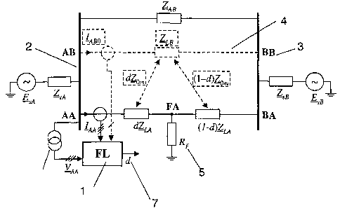
Fig.1 presents a schematic diagram for one-end fault location
applied for parallel lines and for a power transmission or
distribution system with a single line. A fault locator 1 is
positioned at one end 2 of a single line AA-BA 3 or parallel
lines AA-BA, AB-BB, 4. A fault F is shown at FA with a
corresponding fault resistance, 5, denoted as RF . A value for
distance to the fault d from one end 2 determined and provided
by the fault locator 1 is indicated with the reference number
7. Components such as parallel line AB-BB and quantities such
as a parallel line value zero sequence current IABo shown with
dotted lines are excluded when considering a single line case.
The fault locator 1 positioned at the first end 2, or `A' end,
is supplied with the following input signals:
- three-phase voltages (VAA) of the faulted line,
- three-phase voltages (I) of the faulted line,
- zero sequence current (IABO) from the healthy parallel line
(zero sequence is not present when the single line only is
considered).
Fig.2 a,b,c show circuit diagrams of a parallel transmission
network for the positive 2a, negative 2b, and zero sequence 2c
components. Fault loops for the sequence components 21a, 21b,
21c are shown for the case of a fault locator installed at the
terminal AA. An extra link 25 between the terminals A, B is
shown. A generalized model of the fault loop considered for
different fault types is stated as: l
V,1-p-dZ1LIM -RF(aF1IF1+aF2IF2+aFOIFO)-0 (1)
where:
7
CA 02489178 2004-12-09
WO 2004/001431 PCT/SE2003/001091
d - unknown and sought distance to fault,
Z1LA - positive sequence impedance of the faulted line,
VAA-P, I,A_P - fault loop voltage and current composed according
to the fault type,
RF - fault resistance,
IFl - sequence components of the total fault current (i = 0, i
= 1, i = 2),
aFi - weighting coefficients (TABLE 2).
Fault loop voltage and current can be expressed in terms of
the symmetrical components of measured voltages/currents:
VA-P =a1vAA1+a2VAA2+aOVAAO (2)
I na_P =aiLAA1 +a2I AA2 +aO ZOLA IAAO +aoõ: Zo , IABO (3)
Z1LA Z1LA
where:
AA, AB - subscripts used for indicating measurements.
acquired from the faulted line (AA) and from the healthy line
(AB), respectively,
aO, al, a2 - coefficients which are gathered in TABLE 1 (the
Tables are arranged below at the end of the description of
embodiments and derivation of these coefficients is shown in
APPENDIX Al, also attached).
ZOLA, ZOõt - impedance of the faulted line and mutual coupling
between the lines for the zero sequence, respectively,
a o , =aO - for parallel lines,
ao,,, =0 - for single lines.
The phasors of symmetrical components of voltages, positive:
VAAj, negative: V AA2 and zero sequence: VAAO as well as the
phasors of symmetrical components of currents, positive: AA1,
negative: IAA21 zero sequence from the faulted line: IAAO and
zero sequence from the healthy line: IABO are calculated from
8
CA 02489178 2004-12-09
WO 2004/001431 PCT/SE2003/001091
the acquired measurements as shown schematically in schematic
block diagrams Figures 3a and 3b.
Figure 3a shows an input of instantaneous phase voltages 30a,
filtering stage 33a, phasors of phase voltages 31a,
calculation of phasors of symmetrical components 33b and
phasors of symmetrical components of voltages output at 32a.
It may be seen from Fig 3a that acquired phase voltage
measurements are subjected to a filter, then calculations are
made to find the symmetrical components of the fault loop
voltage. Figure 3b shows correspondingly stages used to find
the symmetrical components of the fault loop current. Figure
3b shows instantaneous phase currents and instantaneous zero
sequence current from the healthy line 30b, filtering 33b,
phasors of phase currents and phasor of zero sequence current
from the healthy line 31b, calculation 34b and phasors of
symmetrical components of currents output at 32b.
Fault loop signals may be composed according to formulae (2)-
(3) and TABLE 1, which is the alternative to the classic
approach (TABLE 1A, fault loop voltage (VM-P) and current
(I,-Pwhich was used in the fault locator from [1-2].
Voltage drop across a fault path resistance, the third term in
(1), can be expressed in terms of the current distribution
factors and local measurements of currents which results in:
j1 P-dZ1MIA -RF aF14IAM +a F2IAA2+aFO IMO .0 (4)
kFl kF2 kFo
Formula (4) has been obtained from the following relations
between the symmetrical components of a total fault current
and measured currents:
9
CA 02489178 2004-12-09
WO 2004/001431 PCT/SE2003/001091
I F1 _ AIAA1 I F2 = IAA2 IFO - IAAO
kF1 kF2 kFO
(5)
where:
LF1; 42; kFo - symmetrical components of a total fault
current,
kF1' kF2' kFo - fault current distribution factors for
particular sequence quantities,
AkAA1 = IAA1 , I AA1pre % LAA2 ; IAAO - symmetrical components of
currents measured in the line A at the station A (subscript
AA); note that in case of the positive sequence the
incremental quantity (post-fault current minus pre-fault
current) is used.
Voltage drop across the fault path, as shown in the third term
in equation (1), is expressed using sequence components of the
total fault current. The weighting coefficients aFO' QF1' 1F2'
can accordingly be determined by taking the boundary
conditions for particular fault type. See TABLE 2, Alternative
sets of the weighting coefficients for determining a voltage
drop across the fault path resistance. Examples of derivation
of these coefficients are contained in APPENDIX A2.
There is some freedom for setting the weighting coefficients.
It is proposed to utilize this freedom firstly for avoiding
zero sequence quantities, since the zero sequence impedance of
a line may be considered as an unreliable parameter. This can
be accomplished by setting aFO= O as shown in TABLE 2.
Secondly, the freedom in establishing the weighting
coefficients can be utilized for determining the preference
for using particular quantities. The negative sequence (TABLE
2, set I) or the positive sequence (TABLE 2, set II) can be
CA 02489178 2004-12-09
WO 2004/001431 PCT/SE2003/001091
preferred as well as possibly both types of the quantities
(TABLE 2, set III) can be used for determining the voltage
drop across the fault path.
The set I is recommended for further use, thus avoiding. the
positive sequence, and thus avoiding the pre-fault positive
sequence current, for the largest number of faults. Avoiding
the pre-fault positive sequence current is highly desirable
since sometimes the pre-fault currents - due to certain
reasons - can not be recorded or registered, but may be
contaminated by one or more the symptoms of the occurring
fault. Moreover, the accuracy of recording the pre-fault
currents, which are basically lower than the post-fault
currents, is not very great. This is so since the A/D
converters operate with less accuracy in the low range.
Fault current distribution factors depend on the configuration
of the transmission network, Figures 4, 5, and impedance
parameters. Basically, all impedances for the positive and for
the negative sequence are equal to each other and thus one
obtains:
-F1 =kF2 = K1d + L1 (6)
M1
Coefficients in a fault current distribution factor (6) for a
single (Figure 4) and for parallel lines (Figure 5) are
gathered in TABLE 3, Coefficients for determining a fault
current distribution factor, (note that derivation of the
coefficients is shown in APPENDIX A3).
Figure 4 shows a circuit diagram of a single line for
determining the fault current distribution factor
for the positive sequence currents and with the negative
sequence currents such as shown in brackets. Similarly
Figure 5 shows a circuit diagram of parallel lines for
determining the fault current distribution factor with
11
CA 02489178 2004-12-09
WO 2004/001431 PCT/SE2003/001091
positive sequence currents wherein the negative sequence
currents are shown in brackets.
In Fig.4 the extra link 45 between the terminals A, B having
impedance for the positive sequence equal to: Z1AB can be
considered as existing (Z1AB #-) or as not present (ZIAB _4 )
In Fig.5 the extra link 55 between the terminals A, B having
impedance for the positive sequence equal to: Z1AB can be
considered as existing (Z1LB&AB = ZILBZIAB ) or as not present
Z1LB +Z1AB
( Z1LB&AB - Z1LB) .
Substituting (6) into (4) and adjusting aFp=O (as in TABLE 2)
results in:
VAA p -dZ1LArAA_p - K1dML1 ~F14IAA1 +aF2IAA2)=0 (7)
After multiplying both sides of (7) by: K1d + L1 and some
-AA_p
rearrangements, the quadratic formula with two unknowns, d-
[p.u.] sought fault distance from A, RF - fault resistance, is
obtained:
KlZlLd2+(L1Z1L-KIZAA_p)d-L1ZAA_p+RFM1 ( F1'IAA1+aF2IAA2)=0 (8)
I AA_P
where:
ZAAp= A -p - calculated fault loop impedance.
LAA_p
Writing formula (8) in more compact form results in:
A2d 2 + Ald + A0 + AOORF = 0 (8a)
where:
A2 = A2-Re + JA2_Im = K1Z1LA
Al =A, -R, + jA1_Im = L1Z1LA - K1ZAA p
AO = 40_Re + A -IM = -L1ZAA_P
12
CA 02489178 2004-12-09
WO 2004/001431 PCT/SE2003/001091
A00-R,+ jA d00_Im M1(aF14IAA1+aF2IAA2)
-
I AA-p
ZAA-p = I_-p - calculated fault loop impedance
_p
K1, L1, M1 - coefficients gathered in TABLE 3.
Formula (8a) can be written separately for real and imaginary
parts:
A2_Red2+A1_Red+Ak_Re+AOO_ReRF =0 (8b)
A2 1n,d2+A1_1d+AO_j. +A00_ImRF =0 (8c)
Combining (Sb) and (8c) in such the way that fault resistance
is eliminated [that is, equation (8b) is multiplied by A0o_Im
and equation (8c) by 400_Re and then subtracting them] yields
the quadratic formula for a sought fault distance:
B2d 2 + B1d + B0 = 0 (9)
where:
B2 = A2_ReAOO_Im - A2_I.A00_Re
B1 =A, RAOO h._- Al_ImA00_Re
BO = AO_ReAOO_Im -AO_ImAOO_Re
Equation (9) has two roots (d1, d2) for the distance to fault:
- B1- B12 - 4B2B0
dl = 2B2
- B1 + Bi - 4B2B0
d2 = 2B2
(10)
The root which fulfils the condition (0<- d<1) is selected as
the solution for the distance to fault.
13
CA 02489178 2004-12-09
WO 2004/001431 PCT/SE2003/001091
In another embodiment of the invention, the method of fault
location is carried out by using a measurement of source
impedance at the second end remote from the fault locator 1,
instead of a representative value for the source impedance at
the remote end, and by communicating that measured value to
the local end using a communication means. Coefficients from
(9) are determined with the local measurements and the
impedance data for the transmission line, the extra link
between the line terminals and the equivalent systems at the
line terminals. Impedance of the equivalent system at the
local substation (Z1sA) can be traced on-line with the local
measurements. In contrast, the remote system impedance (Z1sB)
is not measurable locally from A. Thus, the "representative"
value of this impedance may be provided for the algorithm [1-
21.
The alternative solution for the single line case is shown in
Figure 6, which shows a fault locator 1 at the first end 2
near to system A, and another device 10 located at the remote
end 3 close to system B, indicated as RD. A communication
signal 9 is shown being sent from the 10 at the remote end to
the fault locator 1 at the local end.
The remote source impedance (Z1sB) is measured by the remote
device RD, 10, which may be another fault locator or any
suitable device such as a digital relay or digital fault
recorder, in the remote substation and the measurement 9 is
sent via a communication channel 60. Synchronization of
measurements at the line terminals is not required. The source
impedance is calculated from the known relation between the
incremental positive voltage (AVB1) and the incremental
positive sequence current (AIB1) [3-41:
Z1sB dyB1 (11)
dl B1
14
CA 02489178 2004-12-09
WO 2004/001431 PCT/SE2003/001091
Similarly, the fault locator 1 calculates the local source
impedance
Z1sA --AV Al (11a)
AI Al
In another and preferred embodiment of the invention,
compensation is carried out for the shunt capacitance of the
line. Compensation for shunt capacitances effect can be
accomplished by taking into account the lumped model (only the
longitudinal R-XL parameters are taken into account) or the
distributed long transmission line model. The distributed long
line model [5] as providing higher accuracy of fault location,
has been considered here.
The compensation for the single line is presented further.
This means that when composing fault loop current (3) the term
reflecting the mutual coupling effect disappears (a01=O ).
Moreover, the single subscript (A instead of AA) is used.
Fault location procedure with compensating for shunt
capacitances of a transmission line requires the following
additional input data:
CiL - shunt capacitance of a whole line for the positive and
the negative sequences (parameters of a line for the positive
and the negative sequences are identical and thus: C2L- C1L)
COL - shunt capacitance of a whole line for the zero sequence,
l - total line length (km), used for expressing
impedances/capacitances of the line per km length.
The compensation of shunt capacitances may be introduced while
determining the voltage drop across the faulted line segment -
the second term in the generalized fault loop model (1). This
requires compensating the components of the calculated
currents for particular sequences. Thus, the original measured
CA 02489178 2004-12-09
WO 2004/001431 PCT/SE2003/001091
currents: IAi, ZA2, LAO have to be replaced by the currents
after the introduced compensation: I Al-comp , 1 A2_contp I LAO-'Comp
At the same time the original fault loop voltage, the first
term in the model (1), is taken for a distance to fault
calculation. As concerns determining the voltage drop across
the fault resistance, the third term in (1), it is assumed
here, which is a standard practice, that the effect of line
capacitances at the location of the fault (point F), may be
neglected. This is justified as the impedance of the
capacitive branch at that location is much greater than the
fault resistance. This means that the voltage drop across the
fault resistance is determined without taking into account the
shunt capacitances.
Calculating a distance to fault the following impedances
(defined below) are taken as:
ZiL~ - positive sequence impedance of a line with taking into
account the distributed long line model,
ZOLg - as above, but for the zero sequence.
The compensation procedure requires iterative calculations,
performed until the convergence is achieved (i.e. iterated
until the location estimate ceases to differ from the previous
estimate). However, the studies conducted revealed that
results of acceptable accuracy may be obtained using a fixed
number of iterations, for example, 2-3 iterations. The
calculated distance to a fault from a particular (say, present
iteration) is utilized for determining the shunt current in
the next iteration. The determined shunt current is then
deduced from the measured current. A distance to fault,
calculated without considering the shunt effect (10), is taken
as the starting value for the first iteration.
16
CA 02489178 2004-12-09
WO 2004/001431 PCT/SE2003/001091
A way of conducting the first iteration of the compensation is
shown in Figures 7, 8, 9 for the positive sequence, negative
sequence and zero sequence respectively with taking into
account the shunt capacitances effect.
As a result of performing the first iteration for the positive
sequence (Figure 7) the compensated current I A1_comp_1 is
calculated and the last index in the subscript denotes the
first iteration. The calculation is based on deducing the
shunt current from the calculated positive sequence current 'Al
calculated from the measured phase currents - Fig.2:
I A1_comp_l = I Al - 0.5dvlBlLAtanh1 Al (12)
where:
dõ - distance to fault calculated without taking into account
the shunt capacitance effect (10),
1 - total line length (km)
tanh( l O.5Z1LB1Ldvl~
Atanh 1 - \
0.5Z1LB1Ldvl
B1L=J l1L - positive sequence admittance (capacitive) of a
line per km length (S/km)
ZiL= ZIL - positive sequence impedance of a line per km length
(il/km)
Positive sequence impedance of a faulted line segment,
between points A and F, without taking into account the shunt
capacitances effect and considering the lumped line model
equals:
dvlZ1L (13)
while for the considered here distributed long line model:
dvlZiLAsinhl (14)
17
CA 02489178 2004-12-09
WO 2004/001431 PCT/SE2003/001091
where: r
sinhl Z1LB1Ldvi)
Asinh 1 - \ , ,
Z1LB1Ldvi
Thus, the positive sequence impedance of a line with taking
into account the distributed long line model (Zr) equals:
Zlong
1L - AsinhIZ1L (15)
As a result of performing the first iteration for the negative
sequence (Figure 8) the compensated current IA2_co,np_1 is*
calculated and the last index in the subscript denotes the
first iteration. This is based on deducing the shunt current
from the calculated negative sequence current IA2, calculated
from the measured phase currents - Fig.2):
IA2_comp_1 =LA2 -0.5dvlB2LAtanh2VA2 (16)
where, taking into account that the line parameters for the
positive and for the negative sequences are identical
( C2L - C1L , Z2L - Z1L) :
Atanh 2 -" Atanh 1
B 2L - B1L
As a result of performing the first iteration for the zero
sequence (Figure 9) the compensated current LAO-comp-1 is
calculated, last index in the subscript denotes the first
iteration. This calculation is based on deducing the shunt
current from the calculated zero sequence current IAO,
calculated from the measured phase currents - Fig.2:
LAO-comp-1 -LAO -O.5dv1BOLAtanhOVAO (17)
where:
18
CA 02489178 2004-12-09
WO 2004/001431 PCT/SE2003/001091
tanh( 0.5ZoLBoLdVl )
AtanhO - \ ,
0.5ZOLBOLdVl
oL_Jw~oL - zero sequence admittance (capacitive) of a line
per km length (S/km)
ZoL= ZOL - zero sequence impedance of a line per km length
(52/km)
Zero sequence impedance of a faulted line segment, that is
between points A and F, without taking into account the shunt
capacitances effect and considering the lumped line model
equals:
dõIZOL (18)
while for the considered here distributed long line model:
dvlZOLAsinh0 (19 )
where:
sinh/
l ZOLkOLdVl)
Asinh0 - \ ,
FOLBOLdvl
Thus, the zero sequence impedance of a line with taking into
account the distributed long line model (Zr) equals:
Zlwag - OL - AsinhOZ OL (20)
The quadratic complex formula (8) with two unknowns
(dc0mp-1 [p.u..) -- sought fault distance, RF - fault resistance)
after introducing the compensation (first iteration) takes the
following form: ~a
K Zlon dcornp 2 + L Zlong - K Zcomp_1 d L Zco..P-1 +RF- MI FI4I AA1 +aF2-~AA2)
=0
1-L _1) (--1-L 1-A_p comp-1 -1-A_p Icomp_1
-A-p
(21)
19
CA 02489178 2004-12-09
WO 2004/001431 PCT/SE2003/001091
where:
Ztong sinhl Z1LB1Ldvl J
1L - `4sinh1Z1L' `4sinh1 = i
Z1LR1L dvl
ZA"p-1 = oM-p1 - fault loop impedance calculated with:
I p-
-A-p
VA_p - original fault loop voltage (2),
Icomp_1 a I +a I +a I - fault loop -A-p -1-A1_comp_1 -2-A2-coinp_1 -O-AO-comp-
1 current
composed of the positive (12), negative (16) and zero (17)
sequence currents obtained after deducing the respective
capacitive currents from the original currents.
Writing (21) in a more compact form results in:
Acomp _1(d 2 +Acompd +Acornp_1 +Acornp-1R =O
con1p -1 -1 COMP-1 -0 -00 F (21a)
where:
A2 mp _ 1 - Ago Re 1 + Acomp _ 1 - K Z long
J 2-Im -1-1L
comp-1 - Acomp_1 + Acomp_1 = L Z10119 - K Zcomp_1
Al - 1-Re 1-In -1-1L -1-A_p
comp_' dcomp- 1 comp_1 - comp-1
AO - "0_ Re + JAA_ Im - -L1 ZA p
Acomp_1 - dd comp-1 + comp-1 - M 1 (a F1d1 AAl + aF2I AA2 )
-00 - "00_ Re JIAOO_ Im comp
1
A_p
Zcom -1 = YA pl - fault loop impedance calculated with:
I p-
A_p
VA_p - original (uncompensated) fault loop voltage (2),
Icomp- =a I +a I +a I - fault loo current
-A-p -1-Al_comp_1 -2-A2_conip_1 -O-AO_comp_1 p
composed of the positive (12), negative (16) and zero (17)
sequence currents obtained after deducing the respective
capacitive currents from the original currents,
K1, L1, M1 - coefficients gathered in TABLE 3.
Formula (21a) can be written down separately for real and
imaginary parts:
CA 02489178 2004-12-09
WO 2004/001431 PCT/SE2003/001091
com _ 1 2 corn 1 com -I ecom _ 1
Re (dco,np_1) +`41_Re- dcomp_1 +~Re +"00Re RF =0 (21b)
Acomp 2 + Aco rp _ ld + A ' 1 + "Ocomp
m 1RF = 0 (21 c )
2_hn (d comp _1) 1-IM comp _1 _
Combining (21b) and (21c) in such the way that fault
resistance is eliminated, that is, equation (21b) is
multiplied by Aoo'npl,,-,1 and equation (21c) by "00-Re1 and then
subtracting them, yields the quadratic formula for a sought
fault distance:
B2omp_1(d 2 +Bcomp-ld +Bcomp_1 =0 (22)
comp _ 1) 1 comp _ 1 0 -
where:
B comp _ 1 -A comp _ 1 dd comp _1 - Acomp _ 1 comp _ 1
2 - 2-Re "00_Im 2_Im "00-Re
B comp _ 1 -Acomp _ 1/~ comp _ 1 - Acomp _ 1 comp _ 1
1 - 1_Re "00_Im 1_Im "00-Re
Bcomp_1 - comp_1Aoomp_1 - Acon 1AOc0OniP_1
0 - "O _Re 0-In _
Equation (22) has two roots [ (dcornp_1)1 , (dco,np_1)21 for the
distance to fault:
- Blcomp _ 1 - (B1 omp _ 1) 2 - 4B cOmp _ 1BOco,np _ 1 2
(dcomp_1)1 - 2BcO'np_l
2 (23)
-B1omp_1 + (Biomp_1)2 -4B2wnp_1B0comp_1
(d comp _ 1) 2 2B~omp _ 1
The root, which corresponds to the selected previously root
(10) for d (uncompensated) is taken as the valid result. The
compensation procedure requires iterative calculations,
performed until the convergence is achieved (i.e. until the
location estimates cease to change from the previous
estimates) or as with a fixed number of iterations such as 2-3
iterations. The calculated distance to a fault from a
particular (say, present iteration) is utilized for
determining the shunt current in the next iteration.
21
CA 02489178 2004-12-09
WO 2004/001431 PCT/SE2003/001091
The method of the invention is illustrated in two flow-charts
of the FL algorithm, Figure 10, single line and in Figure 11,
parallel lines.
As shown in the flowchart in Figure 10 the following
measurements are utilized:
- voltages from the side A from particular phases a, b, c:
VA_a , VA_b, VA_c
- currents from the side A from particular phases a, b, c: 'A a
1A-b , 1A_c
The input data utilized at step 101, Input data and
measurements, are as follows:
- impedances of the line for the positive (Z1L) and zero (ZoL )
sequences,
- impedance of the extra link 25, 45, 55 between the
substations A, B for the positive (negative) sequences (Z1AB)
- source impedances for the positive (negative) sequences
( Z1sA , Z1,B) : the representative values or the measured values
are used, and a communication means is used for sending the
measured remote source impedance as previously described,
- information on the fault type (from the protective relay).
The measured fault quantities (voltages and currents) undergo
adaptive filtering at step 104, Adaptive filtering of phase
quantities, aimed at rejecting the dc components from currents
and the transients induced by Capacitive Voltage Transformers
(CVTs).
In the next step the symmetrical components of voltages and
currents are calculated, step 105, which is equivalent to that
as shown in Figures 3a, 3b. The fault loop signals are
22
CA 02489178 2004-12-09
WO 2004/001431 PCT/SE2003/001091
composed: the fault loop voltage as in (2), while the fault
loop current as in (3) - but with taking a0222 = 0 .
The distance to fault without taking into account the shunt
capacitances effect (d) is calculated at step 106 by solving
the quadratic formula (9). The solution of (9) is presented in
(10).
The result obtained without taking into account the shunt
capacitances effect d following 106 is treated as the starting
value for performing the compensation for shunt capacitances.
The distributed long line model is applied for the
compensation.
The following additional data is required for the calculating
the compensation for shunt capacitance, step 107:
- positive sequence capacitance of the line (C1L)
- zero sequence capacitance of the line (COL)
- line length (1), which is used to express line impedances /
capacitances per km length.
The first iteration of the compensation leads to the quadratic
equation (22), which is solved in (23). The next iterations
are performed analogously. Iterative calculations are
performed until the convergence is achieved or a fixed number
of iterations, i.e. 2-3 iterations, may be made. The
calculated distance to a fault from a particular (say, present
iteration) is utilized for determining the shunt current in
the next iteration. After completing the iterative
calculations the distance to fault dc0222j1 is obtained.
As shown in the flowchart in Figure 11 for parallel lines the
following measurements are utilized:
- voltages from the side A and line LA from particular phases
a, b, c: vAA-a , VAA-G, vv-AA_c
23
CA 02489178 2004-12-09
WO 2004/001431 PCT/SE2003/001091
- currents from the side A and line LA from particular phases
a, b, c: iAA-a , iAA_b , iAA_c
- zero sequence current from the healthy parallel line LB: iABO
The input data utilized in step 111, Input data and
measurements, are as follows:
- impedances of the faulted line for the positive (Z1LA) and
zero (ZOLA) sequences
- impedance of the healthy line for the positive (negative)
sequence (Z1LB )
- impedance of the extra link between the substations A, B for
the positive (negative) sequences
(Z1AB )
- zero sequence impedance for the mutual coupling (Zoõ,)
- representative values of the source impedances for the
positive (negative) sequences
( Z1sA , Z1sB )
- information on the fault type is obtained from the
protective relay.
The measured fault quantities, the voltages and currents,
undergo adaptive filtering at step 114 for the purpose of
rejecting the dc components from currents and the transients
induced by Capacitive Voltage Transformers (CVTs).
In the next step 115 the symmetrical components of voltages
and currents are calculated as shown in Figures 3a, 3b. The
fault loop signals are composed: the fault loop voltage as in
(2), while the fault loop current as in (3) - but with taking
a0m . a0 .
The distance to fault without taking into account the shunt
capacitances effect (d) is calculated in step 116 by solving
24
CA 02489178 2004-12-09
WO 2004/001431 PCT/SE2003/001091
the quadratic formula (9). The solution of (9) is presented in
(10).
The result obtained without taking into account the shunt
capacitances effect (d) is treated as the starting value for
performing the compensation for shunt capacitances. The
distributed long line model is applied for the compensation.
The following additional data for the faulted line is required
for the compensation for shunt capacitances step 117:
- positive sequence capacitance of the line (CIL)
- zero sequence capacitance of the line (COL)
- line length (1), which is used to express line impedances /
capacitances per km length.
In the case of a single line, the compensation is performed
analogously. Iterative calculations are performed until the
convergence is achieved or by using a fixed number of
iterations, e.g. 2-3 iterations. The calculated distance to a
fault from a particular iteration, for example the present
iteration, is utilized for determining the shunt current in
the next iteration. After completing the iterative
calculations the distance to fault dcornp is obtained.
Figure 18 shows an embodiment of a device for determining the
distance from one end, here shown as end A of a section of
power transmission or distribution line A-B, to a fault F on
the power line according to the method of the invention
described. The fault locator device 1 receives measurements
from measuring devices located at one end A such as current
measuring means 14, and voltage measurements from voltage
measurement means 11. The fault locator device may comprise
measurement value converters, members for treatment of the
calculating algorithms of the method, indicating means for the
calculated distance to fault and a printer or connection to a
printer or facsimile machine or similar for printout of the
CA 02489178 2004-12-09
WO 2004/001431 PCT/SE2003/001091
calculated fault. In a preferred embodiment of the device the
fault locator comprises computer program means for providing a
display of the information provided by the method of the
invention, such as distance to a fault d or dcoõq, on a terminal
which may be remote from the location of the line and/or the
fault locator. Preferably the computer program means receives
information from the fault locator and makes it available to
provide information for a display of a computer such that an
operator or engineer may see a value for the calculated
distance to a fault displayed. The value may be displayed
relative to a schematic display of the line or network in
which the fault has taken place.
In the embodiment shown, measuring device 14 for continuous
measurement of all the phase currents, and measuring device 11
for measurement of voltages are arranged at one end, station
A. Optionally, measuring devices such as 15, 13 may also be
arranged at station B but they are not necessary to practise
the invention. The measured values such as: the three-phase
voltages (VAA) of the faulted line, three-phase voltages (-TA,)
of the faulted line and zero sequence current (IABo) from the
healthy parallel line (note that zero sequence is not present
when the single line only is considered), and a value
representative of the source impedance at B, Z1SB as a are all
passed to a calculating unit comprised in fault locator 1,
filtered such as described in relation to figure 3a, 3b, and
stored in memory means. The calculating unit is provided with
the calculating algorithms described, and programmed for the
processes needed for calculating the distance to fault.
Optionally, the source impedance for the remote end, Z1SB may
be measured by the remote device RD, 10, and the information
sent via a high speed communication means 60 to the fault
locator at A. In some applications it will be preferable to
use a measured value sent from B instead of a representative
value stored at A. It may be seen in Figure 18 that current
26
CA 02489178 2004-12-09
WO 2004/001431 PCT/SE2003/001091
measuring means 15 and voltage measuring means 13 at remote
end B may provide a RD 10, a fault locator, or any suitable
device with measurements to calculate the remote source
impedance
The calculating unit of fault locator 1 is provided with pre-
fault phase currents and also with known values such as shunt
capacitances and the impedances of the line. In respect of the
occurrence of a fault, information regarding the type of
fault, phase-to-phase, phase-to-ground etc., may be supplied
to the calculating unit of the fault locator. When the
calculating unit has determined the distance to fault, it is
displayed on the device and/or sent to display means which may
be remotely located. A printout or fax of the result may also
be provided. In addition to signalling the fault distance, the
device can produce reports, in which are recorded measured
values of the currents of both lines, voltages, type of fault
and other measured and/or calculated information associated
with a given fault at a distance.
The method and a fault locator device according to any
embodiment of the invention may be used to determine distance
to a fault on a section of power transmission line. The
present invention may also be used to determine a distance to
a fault on a section of a power distribution line, or any
other line or bus arranged for any of generation,
transmission, distribution, control or consumption of
electrical power.
The fault locator device and system may comprise filters for
filtering the signals, converters for sampling the signals and
one or more micro computers. The microprocessor (or
processors) comprises a central processing unit CPU performing
the steps of the method according to the invention. This is
performed with the aid of a computer program, which is stored
27
CA 02489178 2004-12-09
WO 2004/001431 PCT/SE2003/001091
in the program memory. It is to be understood that the
computer program may also be run on one or more general
purpose industrial computers or microprocessors instead of a
specially adapted computer.
The computer program comprises computer program code elements
or software code portions that make the computer perform the
method using equations, algorithms, data and calculations
previously described. A part of the program may be stored in a
processor as above, but also in a ROM, RAM, PROM or EPROM chip
or similar. The program in part or in whole may also be stored
on, or in, other suitable computer readable medium such as a
magnetic disk, CD-ROM or DVD disk, hard disk, magneto-optical
memory storage means, in volatile memory, in flash memory, as
firmware, or stored on a data server.
A computer program according to the invention may be stored at
least in part on different mediums that are computer readable.
Archive copies may be stored on standard magnetic disks, hard
drives, CD or DVD disks, or magnetic tape., The databases and
libraries are stored preferably on one or more local or remote
data servers, but the computer program and/or computer program
product may, for example at different times, be stored in any
of; a volatile Random Access memory (RAM) of a computer or
processor, a hard drive, an optical or magneto-optical drive,
or in a type of non-volatile memory such as a ROM, PROM, or
EPROM device. The computer program may also be arranged in
part as a distributed application capable of running on
several different computers or computer systems at more or
less the same time.
in another preferred embodiment, the fault locator may be used
with parallel lines to locate single phase-to-ground faults
(a-g, b-g, c-g faults) in case of unavailability of
28
CA 02489178 2004-12-09
WO 2004/001431 PCT/SE2003/001091
measurements from the healthy parallel line. Two modes of the
healthy line operation are taken into account:
- the healthy line being in operation,
- the healthy line switched-off and grounded at both the ends.
Figure 19 shows the flow-chart of the algorithm for locating
faults in parallel lines under unavailability of measurements
from the healthy parallel line. The unavailable, here healthy
line zero sequence current, is required for reflecting the
mutual coupling effect under single phase-to-ground faults (a-
g, b-g, c-g faults). The unavailable current is thus
estimated. The other faults can be located with the standard
fault location algorithm (such as the algorithm from reference
[ 1 ])
The sequence of computations for the presented one-end fault
location algorithm is as follows.
As shown in the flowchart in Figure 19 the following
measurements are utilized:
- voltages from the side A and line LA (faulted) from
particular phases: vAA-a , v,yA-b vAA_c
- currents from the side A and line LA (faulted) from
particular phases: iffy-, , iAA_b , 'AA -c
The utilized input data are as follows:
- impedances of the faulted line for the positive (Z1LA) and
zero (ZOLA) sequences
- impedance of the healthy line for the zero sequence (ZoLB)
- zero sequence impedance for the mutual coupling (ZO,n)
- information on the fault type (from the protective relay)
- mode of the healthy line operation: in operation or
switched-off and grounded at both ends).
The measured fault quantities (voltages and currents) undergo
adaptive filtering aimed at rejecting the dc components from
29
CA 02489178 2004-12-09
WO 2004/001431 PCT/SE2003/001091
currents and the transients induced by Capacitive Voltage
Transformers (CVTs).
The following equations are used in the method of the present
parallel line embodiment. In addition to the algorithm (1)
described above,for estimating distance to fault (d [pu]) by
considering the Kirchhoff's voltage law for the fault loop as
seen from the locator installation point:
V -dZ I R aF1d7AA1 +aF21AA2 +,aFOIAAO J=O (24)
AA_p -1LA-AA_p _`F kFl kF2 kF0
the fault loop voltage (V,A_p) and current (IM_p) can be
expressed in terms of the symmetrical quantities:
VAA_p-a1VAA1+a2VAA2+a0VAAO (2)
and
SL Zorn
IAA -p =IAAp+Z1LA IABO (25)
where:
I_p-a1IAA1+a2IAA2+aoZOLA IAAO (25a)
-AA Z1LA
is the fault loop current without compensating for the mutual
coupling effect (i.e. composed as for the single line -
superscript SL),
a1, a2, ao- complex coefficients gathered in TABLE 1 (the
derivation as in APPENDIX Al),
V,A1 , V,A2 , V AAO - positive, negative and zero sequence -of
measured voltages,
IAA1 ' I AA2 ' I AAo - positive, negative and zero sequence current
from the faulted line LA,
IABO - unavailable zero sequence current from the healthy
parallel line LB (to be estimated),
CA 02489178 2004-12-09
WO 2004/001431 PCT/SE2003/001091
Z1LA , Zoza - positive and zero sequence impedance the whole
line LA,
Z0M - zero sequence impedance for mutual coupling between the
lines LA and LB,
RF - unknown fault resistance.
In the next step the symmetrical components of voltages and
currents are calculated as shown in Figures 3a, 3b. The fault
loop signals are composed: the fault loop voltage as in (2),
while the fault loop current as in (25). The formulae (2)-(25)
present the fault loop signals expressed in terms of the
symmetrical components of the measured signals. However, one
can use the classic way for composing the fault loop signals.
The presented method covers single phase-to ground faults (a-
g, b-g, c-g faults). The other remaining faults have to be
located with the fault location algorithms described above or
standard fault location algorithm [1]. Distance to fault (d)
for the considered here single phase-to ground faults is
calculated by solving the quadratic formula for a sought
distance to fault (26). Equation (26) is the same as equation
(10) except that the values for B1,B2,B3 are different to the
values determined in (10). The solution gives two roots:
- B1- B1 - 4B2Bo
d1 2B2
(26)
- B1 + Bl - 4B2B0
d2 = 2B2
(as above, the root which fulfils the condition (0<d<_ 1) is
selected as the solution for the distance to fault). One has
to substitute the following into (26):
B2 = real(A2) imag(A00) - real(A00) imag(A2)
B1 = real(A1) imag(A00) - real(A00) imag(A1)
31
CA 02489178 2004-12-09
WO 2004/001431 PCT/SE2003/001091
BO = real(A0) imag(A00) - real(A00) imag(Ao )
where:
SL Z" ZOna
A2= -Z1LAKIIAA_P K1IAAO - QO
Po Po
Al = K1V AA_P - Z1LALII SL AA_p - 1 Z,Om L1IAAo
o
Ao = L1KM_P
A00 =-M1aF2IAA2
QO M 1( F1d1 AA1 +-F2I AA2
The recommended SET of the coefficients b Fl,bF2 are taken from
TABLE 4 and the recommended SET of the coefficients a F11 aF21
!FO from TABLE 5.
Fault loop voltage in this embodiment is found from the TABLE
below
Fault loop voltage composed Fault loop voltage composed
in terms of symmetrical as in the classic approach
components
V AA_P =a1VAA1 +a2V AA2 +aOV AAO
a-g fault: a1 =a2 =a0 =1 a-g fault: VAA_P =KAA_,,
b-g fault: al=q. 2 a2=a, a0=1 a-g fault: VAy_P =KAA-b
2 a-g fault: VAA_P =KAA_,
c-g fault: g1-g, a2=a , ao=1
a=exp(j2)r /3), j=V 1
Fault loop current IPcomposed as for the single line is
found from the TABLE below
32
CA 02489178 2004-12-09
WO 2004/001431 PCT/SE2003/001091
IAA_P in terms of symmetrical I,S~LP as in the classic approach
components
SL Z OLA
IAA_p =a1IAA1 +a2IA42 +a0 IAAO
Z1LA
a-g fault: a1 =a.2 a.
a-g fault: ISL -I +koI
-AA_p -AA_a --AAo
b-g fault: a 2
1 =a a2 =a , a a-g fault: ISL -I +kOI
-AA-P = -AA_a -AAO
c-g fault: a1 =a, a2 =a , go= 1 SL
2
a-g fault: IAA_P =L a +koIAAo
a=exp(j2)r/3), j=
where : k 0 = LA - Z1LA
Z1LA
The complex coefficients dependent on the mode of the healthy
parallel line operation:
a) healthy line LB is in operation:
__ ZOLB -ZOin
P ZOLA -Z0,n
K1 = -Z1LA (Z1sA +Z1sB +Z1LB
Ll = -K1 +Z1LB Z1SB
M1 =Z1LAZILB+ZILA(ZlSA+Z1SB)+Z1LB(Z1SA+Z1SB)
b) healthy line LB is switched-off and grounded:
PO ZOLB
--
ZO,n
K1 - -Z1LA
L1 =Z1LA +Z1sB
M 1 = Z1sA + Z1sA + Z1LA
33
CA 02489178 2004-12-09
WO 2004/001431 PCT/SE2003/001091
In another embodiment, which is presented here, the method is
applied for the standard availability of the measured signals
and is only valid for ground faults, including both:
- single phase-to-ground faults
- phase-to-phase-to-ground faults.
Fault location procedures obtained for these faults under the
standard availability of the fault locator input signals are
extremely simple and compact. Distance to a fault is
calculated with a first order formula.
Figure 22 shows a flow-chart of the developed algorithm for
locating ground faults in parallel transmission lines.
The sequence of computations for the presented one-end fault
locator is as follows. As shown in the flowchart in Figure
22.B3 the following measurements are utilized:
- voltages from the side A and line LA from particular phases
a, b, c: VM_a , VAA_b , !AA-c
- currents from the side A and line LA from particular phases
a, b, c : lAA_ a , iAA-b , iAA_ e
- zero sequence current from the healthy parallel line LB: iAB0
The utilized input data are as follows:
- impedances of the faulted line for the positive (Z1LA) and
zero (ZOLA ) sequences,
- impedance of the healthy line for the zero sequence (ZoLB)
- zero sequence impedance for the mutual coupling (Zorn)
- information on the fault type from the protective relay.
The measured fault quantities (voltages and currents) undergo
adaptive filtering aimed at rejecting the dc components from
currents and the transients induced by Capacitive Voltage
Transformers (CVTs), preferably as described and shown in
relation to Figures 3a, 3b.
34
CA 02489178 2004-12-09
WO 2004/001431 PCT/SE2003/001091
A generalized model of the fault loop, used for deriving the
algorithm of the present embodiment, is stated as follows:
vAA-p-dZ1LAIAA-p-RFCaF1IF1+aF2IF2+aFOIFO)=0 (1)
where:
d - unknown and sought distance to fault,
Z1LA - positive sequence impedance of the faulted line,
KAA-p,IAAp - fault loop voltage and current composed according
to the fault type,
RF - fault resistance,
IFZ - sequence components of the total fault current (i=0 -
zero sequence, i=1 positive sequence,
i=2 - negative sequence),
aFj - weighting coefficients (TABLE 2).
Fault loop voltage and current can be expressed as in classic
distance protection technique or, as in this document, in
terms of the local measurements and with using the
coefficients (a0, a1, a2) which are gathered in TABLE 1
(derivation of the coefficients is contained in APPENDIX
APP.1):
VAAp =a1VAA1+a2VAA2+a0VAA0 (2)
IAA _ p = a1IAA1 + a2IAA2 + aO ZOLA IAAO + a0 ZOni I ABO (3)
Z1LA Z1LA
where:
AA, AB - subscripts used for indicating measurements acquired
from the faulted line (AA) and from the healthy line (AB),
respectively,
ZOLA, Zofn - impedance of the faulted line and mutual coupling
between the lines for the zero sequence, respectively.
In the next step the symmetrical components of voltages and
currents are calculated as shown in Figure 3a, 3b. The fault
CA 02489178 2004-12-09
WO 2004/001431 PCT/SE2003/001091
loop signals are composed: the fault loop voltage as in (2),
while the fault loop current as in (3). The formulae (2)-(3)
present the fault loop signals expressed in terms of the
symmetrical components of the measured signals. However, one
may instead use the classic way for composing the fault loop
signals, as shown in APPENDIX Al.
The presented method covers single phase-to ground faults (a-
g, b-g, c-g faults) and phase-to-phase-to-ground faults (a-b-
g, b-c-g, c-a-g faults), thus, the faults for which the
highest fault resistance can be expected. The other remaining
faults have to be located with the fault location algorithms
described above or a standard fault location algorithm, such
as for example the fault locator from reference [1]).
Distance to fault (d) for single phase-to-ground faults is
calculated as follows:
a-g fault:
imag{V,A_p[3(IMo -I'oI ABO)]*}
(27a)
iniag {(Z1LAIAA_p)[3(IAAO -PoI ABO)]*}
where:
Fault loop signals composed Fault loop signals composed
in terms of symmetrical as in the classic approach
components
VAA_p =a1VAA1+a2VAA2+aOVAAO YAA-p =VAA-a
IAA_p =a1LAA1+a2IAA2+
ZOLA
+ao z IAAO+ao Zo,n IABO IAA-p =LAA_a+koIAAO+koõ,IABo
Z1LA Z1LA
where : al = a2 = ao =1 where : k ZOLA - Z1LA k Zonz
Z1LA Oin Z1LA
ZOLB - ZO,n
Po = (for symmetrical lines: Po =I).
ZOLA _ ZO,n
b-g fault:
36
CA 02489178 2004-12-09
WO 2004/001431 PCT/SE2003/001091
d - imag{V~_P[3a 2 (I,Ao -PoIABO)]*} (27b)
imag{(ZILAIAA-P)[3a2(IAAO -PoIABO)]*}
where:
Fault loop signals composed Fault loop signals composed
in terms of symmetrical as in the classic approach
components
V AA_ p = a1 Yi AA1 + a 2V AA2 + aOV AAO V AA- p = V AA- b
IAA_p a1IAA1+a2IAA2+
+ao ZOLA IA4O +ao Zom LABO IAA-p -IAA-b +koLAAO +komiABO
Z1LA Z1LA
where : a1 = a2 2 = a , ao =1 where : ko - ZOLA -Z1LA ko~n = ZOm
- - Z1LA ZiLA
a = exp(j2)C / 3)
ZOLB -Zom
PO = (for symmetrical lines: P 0 1 ) .
ZOLA -Zonz
c-g fault:
imag{VAA_p[3a(IAAO -PoLABO)]*}
(27c)
imag{(ZILAIAA-p)[3a(IAAO -PoLABO)]*}
where:
Fault loop signals composed Fault loop signals composed
in terms of symmetrical as in the classic approach
components
VAA_p =a1VAA1+a2VAA2+aOVAAO VAA_p =VAA_c
IA_p a1IAA1+a2IAA2+
+a.oZO~IAAO+aOZo,n jABO IAA-p=IAA_c+koIAAO+komlABO
Z1LA Z1LA
where : a1 = a , 2 =q 2 , 0 =1 where : ko - ZOLA - Z1LA kona = ZOm
a=exp(j21r/3) - Z1LA Z1LA
ZOLB - ZO a
PO = (for symmetrical lines: PO =1) .
ZOLA - Zom
37
CA 02489178 2004-12-09
WO 2004/001431 PCT/SE2003/001091
Distance to fault (d) for phase-to- phase-to ground faults can
be calculated in two different ways, depending whether the
pre-fault currents can be used or have to be avoided.
1. Procedure for distance to fault calculation with the use of
pre-fault measurements:
a-b-g fault:
d - imag {V ~1 _P I (I AAO - 0I ABO )]* }
ima -
g{(Z-1LAI-AA_p) WI IwAAO POIABo)]*} (28a)
where: W = AAIAA1+BIAA2
- ,
CZIAA1 +DIAA2
A=1-a2 B=1-a , C=1+a2 , D=1+a
Fault loop signals composed Fault loop signals composed
in terms of symmetrical as in the classic approach
components
VAA_p=a1VAA1+a2VAA2+aOVAAO VAA_p=VAA-a-VAA_b
IAA-p =a1I 11+a2IAA2+
+aoO~IAAO+aoo,n IABO IAA p=IAA_a-IAA_b
Z ILA Z1LA
where: a1=1-a2, a2=1-a, ao=0
a =exp(j2z /3)
ZOLB - ZOna
PO = (for symmetrical lines: PO=I).
ZOLA -Z0nz
b-c-g fault:
imag{V,~1_p[(IAAo -PoIABO)]*}
d= * (28b)
imag{(Z1LA AA_p)L(AAo -PoJABO)r }
38
CA 02489178 2004-12-09
WO 2004/001431 PCT/SE2003/001091
where: W= Ad-zAA1+BIAA2 , A=a2-a , B=a-a2, C=-1, D=-1
C4I AA1 + DI AA2 - -
Fault loop signals composed Fault loop signals composed
in terms of symmetrical as in the classic approach
components
VAA_p =a1VAA1 +a2VAA2 +aOVAAO VAA_p =VAA-b -V AA_c
IAA_p =a1IAA1+a2IAA2+
+ao ZOLA I AAO +a0 Z0m I ABO IAA-p =IAA-b -IAA-a
Z1LA Z1LA
where: a1=a2-a, 92=a-a21 a0=0
a=exp(j2)r/3)
ZOLB -ZOnx
PO = (for symmetrical lines: PO =I).
ZOZA - Zorn
c-a-g fault:
d - imag{V,~_prw (IAAO-PoIABO)I }
imag{(Z1LAIAA_ )1W(IAAO -POI (28c)
p --ABO T }
where:
W = A4IAA1+BIAA2
CLIAA1 +DIIAA2
A=a-1 , B=a2-1, C=a+1 , D=a2+1
Fault loop signals composed Fault loop signals composed
in terms of symmetrical as in the classic approach
components
V AA_p = a1V AA1 + a2V AA2 + a0V AA0 VAA_p = VAA-, - VAA_a
IA_p =a1lAA1+a2I,A2+
+aoZOLA IAAO+ao ZOm IABO IAA-p=IAA-IAA-a
Z1LA ZILA
where: a1=a-1, a2=a2-1, a0=0
a =exp(j2)t/3)
39
CA 02489178 2004-12-09
WO 2004/001431 PCT/SE2003/001091
ZOLB - ZOrn
Po = (for symmetrical lines: Po =I).
Z OLA - Z 0,
2. Procedure for distance to fault calculation without the use
of pre-fault measurements:
a-b-g fault:
d= imag[(Va +Vb)(IAAO -P0IAB0)*] (29a)
imag[Z1z.A(Ia +Ib +2koLAAo +2k01 LABO)(IAAo -j'oLABO)*]
b-c-g fault:
d _ imag[(Vb +Vc)(IAAO -PoLABO)*] (29b)
iinag[Z1L1(Ib +I, +2koIAAo +2kornIABO)(IAAo -PoIABO)*]
c-a-g fault:
d _ imag[(Vc +Va)(IAAO -PoLABO)*] (29c)
ilnag [Z1 (L +Ia +2koLAAo +2k07 LABO)(IAAO -PoIABO)*]
where: k0 - ZOLA -Z1LA k0,n = Zorn
Z1LA Z1LA
It is also noted that while the above describes exemplifying
embodiments of the invention, there are several variations and
modifications which may be made to the disclosed solution
without departing from the scope of the present invention as
defined in the appended claims.
CA 02489178 2004-12-09
WO 2004/001431 PCT/SE2003/001091
Tables
TABLE 1. Coefficients for determining the fault loop voltage
(VAA^P) and current (IAA_p) in terms of symmetrical components
as defined in (2) and (3).
Fault type a1 a2 aQ
a-g 1 1 1
b-g a2 a 1
c-g a a2 1
a-b, a-b-g
1-a2 1-a 0
a-b-c, a-b-c-g
b-c, b-c-g a2-a a-a2 0
c-a, c-a-g a-1 a20
a=exp(j2TC/3), j=
TABLE 1A. Fault loop voltage (VAA_P) and current (LAA_p)
expressed with using the classic approach.
Fault type VAA_P AA_p
a-g V AA a LAA_a +koJAAO +komlABO
b-g VAA b IAA_b+kOIAAO+kOrnIABO
c-g VAA_c IAA_, +kOIAAO +kOnzIAB0
a-b, a-b-g VAA_a -VAA_b IAA_a -IAA_b
a-b-c, a-b-
c-g
b-c, b-c-g V AA_b -V AA_c LAA_b - I AA_c
c-a, c-a-g V AA_c -VAA_a IAA_c - I AA_a
k0 ZOLA - Z1LA k0rn - ZO"
- = ' - -
Z 1LA Z1LA
a=exp(j21r13), j=
TABLE 2. Alternative sets of the weighting coefficients for
determining a voltage drop across the fault path resistance
41
CA 02489178 2004-12-09
WO 2004/001431 PCT/SE2003/001091
Set I Set II Set III
Fault (recommended)
type
aFl aF2 aFO aFl 9F2 aFO aFl 9F2 aFo
a-g 0 3 0 3 0 0 1,5 1,5 0
b-g 0 3a 0 3a2 0 0 1,5a2 1,5a 0
c-g 0 3a2 0 3a 0 0 1,5a 1,5a2 0
a-b 0 1-a 0 1-a2 0 0 0,51_a2 0,5(1-a) 0
b-c 0 a-a2 0 a2-a 0 0 0,5a2-a 0,5a_a2 0
c-a 0 a2 -1 0 a-1 0 0 0,5(-1) 0,5 a2 _ 1 0
a-b-g 1-a2 1-a 0 1-a2 1-a 0 1-a2 1-a 0
b-c-g a2 -a a-a2 0 a2 -a a-a2 0 a2 -a a-a2 0
c-a-g a-1 a2 0 a-1 a2 0 a-1 a2 -1 0
a-b-c-g 1-a 2 0 0 1-a 2 0 0 1-a 2 0 0
(a-b-c) - - -
a = exp(j2)r / 3) , j=
TABLE 3. Coefficients for determining a fault current
distribution factor (6)
SINGLE LINE (Fig.4)
K1 = -Z1LZIAB - lZ1sA + -Z1sBB )~Z1L
Z 1AB ,hoc L 1 - Z1L (Z1A + Z1s((lB~~)+Z1AB (111L +Z1sB )
M 1 = 4~' 1sA + Z1SB~(G 1AB +Z1L )+ Z1L ZIAB
K1 =-Z1L I'1 =Z1L+ZLB
Z1AB M1 =Z1sA +Z1sB +Z1L
PARALLEL LINES (Fig.5)
K1 =-ZILA( i1sA+ZIsB +Z1LB&AB)
Z'1 =Z1LA( 1sA +Z1sB +Z1LB&AB)+Z1LB&ABZ1B1
M1 =ZILAZILB&AB +Z1LA(Z1sA +Z1sB)+Z1LB&AB(Z1sA +Z1sB)
where: Z1LB&AB - Z1LB Z1AB
Z1LB +Z1AB
42
CA 02489178 2004-12-09
WO 2004/001431 PCT/SE2003/001091
Table 4 The recommended SET of the coefficients bF1 , bF2 in
relation to (26)
Fault bFl bF2
a-g 0 1
-g 0 a 2
c-g 0 a
a=exp(j2r/3), j=
Table 5 The recommended SET of the coefficients aF1 , aF2 , aFo
in relation to (26)
FAULT a F1 aF2 aFo
a-g 0 3 0
b-g 0 3a 0
C -g 0 3a 2 0
a = exp(j2)r/3), j =
43
CA 02489178 2004-12-09
WO 2004/001431 PCT/SE2003/001091
References
[1] Eriksson L., Saha M.M., Rockefeller G.D.: An accurate fault
locator with compensation for apparent reactance in the
fault resistance resulting from remote-end infeed, IEEE
Transactions on PAS, Vol. PAS-104, No. 2, February 1985,
pp. 424-436.
[2] Saha M.M.: Method and device for locating a fault point on
a three-phase power transmission line. United States
Patent, Patent Number: 4,559,491, Date of Patent: Dec.17,
1985.
[3] McLAREN P.G., SWIFT G.W., ZHANG Z., DIRKS E., JAYASINGHLE
R.P., FERNANDO I., A new positive sequence directional
element for numerical distance relays, Proceedings of the
Stockholm Power Tech Conference, Stockholm, Sweden, 1995,
pp. 540-545.
[4] SAHA M.M., IZYKOWSKI J., KASZTENNY B., ROSOLOWSKI E., PALKI
B.S., Relaying algorithms for protection of series-
compensated lines, Proceedings of the International
Conference on Modern Trends in the Protection Schemes of
Electric Power Apparatus and Systems, October 28-30, 1998,
New Delhi, India, pp. V-50-61.
[5] NOVOSEL D., HART D.G., UDREN E., GARITTY J., Unsynchronized
two-terminal fault location estimation, IEEE Transactions
on Power Delivery, Vol. 11, No. 1, January 1996, pp. 130-
138.
APPENDICES
Al. DERIVATION OF THE COEFFICIENTS a1, a2, ao (TABLE 1)
Single phase-to-ground fault: a-g fault
VAA_p =VAA_a =iAA1 +VM2 +VMO =alV.9A1 +a2V.9A2 +a0Vaa0
44
CA 02489178 2004-12-09
WO 2004/001431 PCT/SE2003/001091
IAA _ p =IAA _ a +k 0 I AA0 + kOin I ABO = I AA1 + I AA2 + I AA0 + Z OLA - Z
1LA I AAO + ZOin I ABO =
Z1LA Z1LA
= I AA1 + I AA2 + ZOLA IAAO + ZOrn I ABO = a1I AAl + a2-AA2 + aO ZOLA IAAO +
a0,,, Z0.. I ABO
Z1LA Z1LA Z1LA Z1LA
Thus: a1=a2=a0=1
Inter-phase faults: a-b, a-b-g, a-b-c, a-b-c-g faults
VAA_p =VAA_a -VAA_b = ((VLAA1 +VAA2 +VAAO) - Ca 2V AAJ +aVAA2 +VAAO)=
_ (1-a2)AA1 +(1-a)V AA2 = 91V AA1 +a2V AA2 +a0VAA0
IAA_p =IAA_a - IAAb =(IAAI+IAA2+IAAO) -Ca 2IA91+aIAA2+IAAO)_
2 ~AAI + (1 - a)I AA2 - a1IAAl + a2I AA2 + a0 ZLO I AAO
ZL1
Thus: a1 =1-a2, a2 =1-a , a0 =0
A2. Derivation of coefficients aF11 9F21 aFO (TABLE 2)
TABLE 2 contains three alternative sets (Set I, Set II, Set
III) of the weighting coefficients, which are used for
determining a voltage drop across a fault path. The
coefficients are calculated from the boundary conditions -
relevant for a particular fault type. This is distinctive that
in all the sets the zero sequence is omitted (aFO= 0). This is
advantage since the zero sequence impedance of a line is
considered as the uncertain parameter. By setting aFO= 0 we
limit adverse influence of the uncertainty with respect to the
zero sequence impedance data upon the fault location accuracy.
To be precise one has to note that this limitation is of
course partial since it is related only to determining the
voltage drop across a fault path. In contrast, while
determining the voltage drop across a faulted line segment the
zero sequence impedance of the line is used.
a-g fault, Figure 12:
CA 02489178 2004-12-09
WO 2004/001431 PCT/SE2003/001091
Taking into account that in the healthy phases: IF_bIF_c 0
what gives: IF11 LF_a+aIF_b+a2IF_c)=1 LF_a+a0+a20)=11F a
3 3 - 3-
1F2 = ~,F_a +a27F_b +aIF_c)=1(IF_a +a2O+aO)= 1IF_a
3 3 3-
IFO =(F-a+IF_b+IF_c)- 111Fa+O+O)=1IF_a
3 3 3
The sequence components are related: I F1 I F2 = I FO and
finally:
IF=IF_a=3IF2, thus: aF1=0, aF2=3, aFO=O (as in the Set I
from Table 2)
or
IF =IF a -3IF1, thus: aFl =3, aF2 =0, aFO =O (as in the Set II
from Table 2)
or
IF =IF_a -1,5IF1+1,5IF2, thus: aFl =1,5 , aF2 =1,5 , aFO =O (as in the
Set III from Table 2)
a-b fault Figure 13a, 13b:
The fault current can be expressed as: IF =IF_a or as:
I F = (IF_a -IF-b)
Taking into account that in the healthy phase: -IF-,=O and
for the faulted phases: IF b= -IF a, what gives:
I F1 = 3 ~ F_a +aIF_b +a2IF_c)- 3 (`-F_a +a( I F_a)+a2O)= 3(1-a)IF
I F2 = 3 I F_a +a2IF_b +g F_c)= 3 IF_a +a2(IF_a)+aO)= 3 (1-a2)LF_a
IFO = 1(IF_a+IF_b+IF_c)- 3(,`-F_a+( IF_a)+O)=0
The relation between IF1 and IF2 is thus:
I(1-a)IF
IF1 = 3 -a = (1-a)
jF2 1 2)I a2
3 F_a
46
CA 02489178 2004-12-09
WO 2004/001431 PCT/SE2003/001091
Finally:
3
IF =IF _a = 1-a2 IF2 =(1-a)IF2
thus: aF1-0, aF2=1-a aFO=0 (as in the Set I from Table 2)
or
_ 3 2lT
IF =IF-a (1-a)-Fl =(1-a )IF1
thus : aF1=1-a2 , aF2 =0 , aFO = 0 (as in the SET 2 from Table 2)
or
IF =0,5IF a+0,5IF-a = 1'52 IF2+ 15 IF1 =0,5(1-a)IF2+0,5(1-a2kF1
-a (1-a)- -
thus: aF1 =0,5(1-a2), aF2 =0,5(1-a) , aFO =0 (as in the Set III
from Table 2)
(a-b-g) fault, Figure 14:
IF =IF_a - IF_b -llF1+IF2+IFO)-(2IF1+aIF2+IFO)
=(1-a2)IF1+(1-a)IF2
Thus: aF1=1-a2, aF2=1-a, aFO=O (as in the Sets I, II, III
from Table 2)
(a-b-c) or (a-b-c-g) symmetrical faults, Figure 15a, 15b, 15c:
Taking the first two phases (a, b) for composing the voltage
drop across a fault path one obtains:
IF IF_a - IF_b =(IF1 +IF2+IF0)-~a 241+aIF2+IFO)
=(1-a2)IF1+11-a)IF2
Thus:
9F1=1-a2, aF2=1-a, aFO=O
Additionally, if a fault is ideally symmetrical the positive
sequence is the only component, which is present in the
signals. Therefore, we have:
47
CA 02489178 2004-12-09
WO 2004/001431 PCT/SE2003/001091
aF1 =1-a2 , aF2 =0 , aFO =0 (as in the Sets I, II, III from Table
2).
A3. Derivation of the complex coefficients in the fault
current distribution factors for the positive (negative)
sequence (Table 3)
a) Case of the single line with extra link 45 between the
substations (Figure 4)
Let us determine the fault current distribution factor for the
positive sequence (the fault current distribution factor for
the negative sequence is the same). The equivalent circuit of
Figure 4 with indicated flow of currents for the incremental
positive sequence is presented in Figure 16.
Considering the closed mesh containing: the local segment of
the faulted line, the remote segment of the faulted line and
the extra link between the substations, one can write down:
dZILA, Al +(1-d)Z1L(AIAl -IF1)-Z1ABAI AB1 = 0
From the above equation the unknown current from the extra
link between the substation can be determined as:
AIAB1 = Z1L (Al Al -(1-d)IFl)
Z1AB
Considering the closed mesh containing the source impedances
(Z1sA ' Z1sB) and the extra link (ZlAB) one can write down :
Z1sA(AIA1 +AIABI)+ZIABAIAB1 +Z1SB(AIAl +AIAB1 -IF1) =0
Substituting the previously determined unknown current from
the extra link into the above equation one obtains:
48
CA 02489178 2004-12-09
WO 2004/001431 PCT/SE2003/001091
kFl dI Al _ Kld + Ll
-
IF1 M1
where, as in TABLE 3 (Single line, Z1AB #-), we have:
K1- -Z1LZIAB -1-IsA + Z1SB )Z1L
Z'1 =Z141sA+Z1sB)+ZIAB(G1L+Z1cB)
M1 =IZIsA +Z1sB)1Z1AB +Z1L)+Z1LZIAB
If there is no extra link between the substations (Z1AB ->') one
has to consider the closed mesh containing the source
impedances (Z1sA, Z1sB) and both the segments of the faulted
line [ dZ1L and (1-d)Z1L ] . For this mesh one can write:
(Z 1sA + d Z 1L )/I Al + [[ lsB + (1- d )Z 1L ](4I Al - I F1) = 0
After rearrangements one obtains:
kFl dlAl _ Kld+Ll
-
I F1 M1
where, as in TABLE 3 (Single line, Z1AB ->-) , we have:
K1 = -ZlL
L =ZlL+Z1SB
M 1 = Z1sA + Z 1sA + Z1L
b) Case of the parallel lines with extra link between the
substation (Figure 5)
Let us determine the fault current distribution factor for the
positive sequence (the fault current distribution factor for
the negative sequence is the same). The equivalent circuit of
parallel lines from Fig.5 with indicated flow of currents for
the incremental positive sequence is presented in Figure 17.
49
CA 02489178 2004-12-09
WO 2004/001431 PCT/SE2003/001091
The healthy parallel line (LB) and the extra link 55 (AB),
which are in parallel connection, have been substituted by the
equivalent branch with the equivalent impedance:
Z1LBZlAB
ZlLB&AB -
Z1LB + Z1AB
Considering the closed mesh denoted by (AA, F, BA, BB, AB) one
can write:
dZlLAJIA1 +(1-d)Z1LA(zIAA1 -IF1)-ZlLB&AB4ILB&AB1 =0
From the above equation the unknown current from the
equivalent branch can be determined as:
AI LB&AB1 = Z1LA (diAA, - (1- d)I F1)
Z1LB&AB
Considering the closed mesh containing the source impedances
( Z1sA , Z1sB) and the equivalent branch (ZlLB&AB) one can write
down:
Z1sA ( I AA1 + I LB&AB1) + Z1LB&AB I LB&AB1 + Z1sB ( I AA1 + AI LB&AB1 - I
F1) = 0
Substituting the previously determined unknown current from
the healthy line into the above equation one obtains:
-Fl - IAA1 _ K1d +L1
I F1 M1
where, a((s~~ in TABLE 3 (Parallel lines), we have :
K1 -Z1LALZ1sA +Z1sB +Z1LB&AB)
Li ZlLA(Z1sA+Z1sB+Z1LB&AB)+Z1LB&ABZ1SB1
M1 =Z1LAZILB&AB +ZILA(ZlSA +Z1SB)+Z1LB&AB(Z1sA+Z1SB)
where : Z1LB&AB ZILBZIAB
Z1LB +Z1AB
In case if the extra link between the substations (Z1AB) is
not present one has to substitute: ZlLB&AB = ZlLB =