Note: Descriptions are shown in the official language in which they were submitted.
CA 02624433 2008-03-07
52925-4 1
A Method and Device for Estimation of the Transmission
Characteristics of a Radio Frequency System
Field of the present invention
The present invention pertains to the field of
radio frequency signalling and electronic countermeasures.
Background of the present invention
Electronic countermeasures (ECM) are a subsection
of electronic warfare which includes any sort of electrical
or electronic device designed to prevent or disrupt
electromagnetic signalling. It may be used both offensively
and defensively. ECM often takes the form of jamming,
whereby a jamming signal is transmitted by an ECM system to
block the reception of other signals within the bandwidth of
the jamming signal. However, in general the jamming signal
has a finite physical area of effect determined by the area
distribution of its radiated energy. Outside this area the
jamming may be only partially effective.
Some types of ECM jamming systems are commonly
used as part of a convoy of vehicles to protect against
hostile use of the electromagnetic spectrum. In these
cases, the ECM jamming system provides a mobile area of
protection against, for example, remote detonation of an
explosive device on or near the convoy's path, while the
convoy passes by. Because microwave energy cannot be sensed
by involved personnel and ECM operators, determining the
real-time, in-situ protection offered by an ECM system is a
problem endemic to the use of ECM.
Summary of the Invention
CA 02624433 2008-03-07
52925-4 2
According to one aspect of the present invention,
there is provided a method comprising the steps of: in a
device physically remote from a radio frequency (RF) system
transmitter: calculating for a first location a predicted
received power level of an RF signal generated by the RF
system transmitter; measuring at the first location an
actual received power level of the RF signal generated by
the RF system transmitter; determining a correction value
based on the predicted received power level and the measured
received power level; and calculating for a second location
a predicted received power level of the RF signal using the
correction value.
In some embodiments, the method further comprises:
calculating for the first location a plurality of predicted
received power levels of the RF signal generated by the RF
system transmitter, inclusive of calculating the first
predicted received power level for the first location,
wherein each one of the plurality of predicted received
power levels corresponds to a respective frequency component
of the RF signal; measuring at the first location a
plurality of actual received power levels of the RF signal
generated by the RF system transmitter, inclusive of
measuring the first actual received power level at the first
location, wherein each one of the plurality of actual
received power levels corresponds to one of the plurality of
predicted received power levels; determining a plurality of
correction values based on the plurality of predicted
received power levels and the plurality of measured received
power levels, inclusive of determining the first correction
value based on the first predicted received power level and
the first measured received power level; and calculating a
plurality of predicted received power levels for the second
CA 02624433 2008-03-07
52925-4 3
location using the plurality of correction values, inclusive
of calculating the first predicted received power level for
the second location using the first correction value.
In some embodiments, the RF signal generated by
the RF system transmitter comprises an electronic
countermeasures (ECM) signal.
In some embodiments, the method further comprises:
predicting probabilistic ability of the RF signal generated
by the RF system transmitter to prevent triggering of a
potential threat device at the second location based on the
predicted received power level of the RF signal at the
second location and potential threat device characteristics.
In some embodiments, the potential threat device
characteristics comprise a predicted response of the
potential threat device to the predicted received power
level of the RF signal at the second location.
In some embodiments, the predicted response of the
potential threat device to the predicted received power
level of the RF signal comprises a predicted response of the
potential threat device to a given jamming-to-signal ratio.
In some embodiments, determining the correction
value comprises calculating the correction value according
to:
API - ECMmea.t'_ at -fir'! - location - ECMrinref _al _.firs/ _ localioli
where API is the correction value, ECMn,eos_m_firv,_/ocaIoõ is the
actual received power level of the RF signal at the first
location, and ECM,f_,,,_firm _/,xe is the predicted received power
level of the RF signal at the first location, wherein
CA 02624433 2008-03-07
52925-4 4
calculating the predicted received RF signal at the second
location comprises: calculating an unrefined predicted
received power level of the RF signal at the second
location; and calculating the predicted received power level
of the RF signal at the second location according to:
El.Mre1_at_second_locaiion = ECMnirej_at - Sec and - location +AP I
where ECM1er_at_secondloca,iS,n is the predicted received power level of
the RF signal at the second location, and ECM,,,,reJ_at_seeond_IKation is
the unrefined predicted received power level of the RF
signal at the second location.
In some embodiments, the method further comprises:
generating a mismatch cost function based on a comparison of
the predicted received power level of the RF signal at the
first location and the actual measured received power level
of the RF signal at the first location; and indicating a
fault/anomaly if the mismatch cost function exceeds a
threshold value.
In some embodiments, the method further comprises:
calculating a respective predicted received power level of
the RF signal generated by the RF system transmitter for
each location of a plurality of locations in an area around
the device using the correction value; and for each location
predicting probabilistic ability of the RF signal generated
by the RF system transmitter to prevent triggering of the
potential threat device at the location based on the
respective predicted received power level of the RF signal
at the location and the potential threat device
characteristics.
CA 02624433 2008-03-07
52925-4 5
In some embodiments, the potential threat device
characteristics comprise a predicted response of the
potential threat device to the respective predicted received
power level of the RF signal for each location of the
plurality of locations in the area.
In some embodiments, the method further comprises
calculating a protection range of the RF system transmitter
by determining a boundary at which the probabilistic ability
of the RF signal generated by the RF system transmitter to
prevent triggering of the potential threat device is at a
safety threshold.
In some embodiments, the method further comprises
displaying the protective range of the RF system
transmitter.
In some embodiments, calculating each respective
predicted received power level of the RF signal comprises:
calculating a predicted received power level of the RF
signal for each location for each one of a population of N
scenario parameter sets to generate N predicted received
power levels for each location, wherein for each location
the probabilistic ability of the RF signal generated by the
RF system transmitter to prevent triggering of the potential
threat device at the location is derived from the
probabilistic effect of the N predicted received power
levels of the RF signal for the location.
In some embodiments, generating the mismatch cost
function comprises determining best-case and worst-case
predicted received power levels of the RF signal at the
first location, wherein the worst-case predicted received
power level of the RF signal at the first location is
CA 02624433 2008-03-07
52925-4 6
derived from N predicted received power levels of the RF
signal at the first location calculated using N scenario
parameter sets, and wherein the best-case predicted received
power level of the RF signal at the first location is
derived from the N predicted received power levels of the RF
signal at the first location.
In some embodiments, the method further comprises,
for each location: determining an average predicted received
power level of the RF signal from the N predicted received
power levels of the RF signal; and determining standard
deviation of the N predicted received power levels of the RF
signal.
In some embodiments, the method further comprises:
predicting a worst-case protection range of the RF system
transmitter; predicting a predicted protection range of the
RF system transmitter; and displaying the worst-case and
predicted protection ranges of the RF system transmitter.
In some embodiments, calculating a predicted
received power level of the RF signal comprises calculating
a predicted received power level of the RF signal using a
propagation and scenario model.
In some embodiments, the method further comprises
adapting parameters of the model to substantially fit the
predicted received power level of the RF signal at the first
location to the measured received power level of the RF
signal at the first location.
In some embodiments, adaptation of the parameters
of the model is accomplished by using an heuristic method to
substantially fit the predicted received power level of the
CA 02624433 2008-03-07
r k
52925-4 7
RF signal at the first location to the measured received
power level of the RF signal at the first location.
In some embodiments, the heuristic method
comprises at least one of: a genetic algorithm, an
evolutionary algorithm, Tabu search, simulated annealing,
and a memetic algorithm.
In some embodiments, the method further comprises:
in the RF system transmitter: transmitting at least one
pilot signal as part of the RF signal, wherein measuring an
actual received power level of the RF signal comprises
measuring an actual received power level of the at least one
pilot signal transmitted by the RF system transmitter.
In some embodiments, at least one of amplitude,
phase, and center frequency of at least one of the at least
one pilot signal is adjusted to determine a set of scenario
model parameters that, for each one of the at least one
pilot signal frequencies, substantially fit the predicted
received power level of the RF signal at the first location
to the measured received power level of the RF signal at the
first location.
In some embodiments, the method further comprises:
in the device: communicating with the RF system to control
the adjustment of the at least one of amplitude, phase and
center frequency of the at least one of the at least one
pilot signal.
In some embodiments, the method further comprises:
estimating uncertainty associated with at least one
parameter of the propagation and scenario model based on
discrepancies between the measured received power level of
the RF signal at the first location and an average predicted
CA 02624433 2008-03-07
52925-4 8
received power level of the RF signal at the first location,
wherein the average predicted received power level of the RF
signal at the first location is derived from a population of
N predicted received power levels of the RF signal at the
first location calculated using N scenario parameter sets.
In some embodiments, only a single pilot signal is
used at any moment and a center frequency of the single
pilot signal is varied across a plurality of frequencies,
wherein the model parameters are adapted to: a)
substantially fit the predicted received power level of the
RF signal at the first location to the measured received
power level of the RF signal at the first location for each
frequency of the plurality of pilot signal frequencies; and
b) estimate uncertainty in at least one model parameter
based on discrepancies between the measured received power
level of the RF signal at the first location and the
predicted received power level of the RF signal at the first
location, where the predicted received power level of the RF
signal is calculated using the adapted set of model
parameters.
According to another broad aspect of the present
invention, there is provided a device comprising: receiver
circuitry that: receives a radio frequency (RF) from an RF
system transmitter physically remote from the device; and
measures a received power level of the RF signal at a first
location; and a processor that: calculates a predicted
received power level of the RF signal at the first location;
determines a correction value based on the predicted
received power level of the RF signal at the first location
and the measured received power level of the RF signal at
the first location; and calculates a predicted received
CA 02624433 2008-03-07
52925-4 9
power level of the RF signal at a second location using the
correction value.
In some embodiments, the RF system transmitter
comprises an electronic countermeasures (ECM) system
transmitter, and the RF signal generated by the RF system
transmitter comprises an ECM signal.
In some embodiments, the processor predicts
probabilistic ability of the RF signal at the second
location to prevent triggering of a potential threat device
at the second location based on the predicted received power
level of the RF signal at the second location and potential
threat device characteristics.
In some embodiments, the potential threat device
characteristics comprise a predicted response of the
potential threat device to the predicted received power
level of the RF signal at the second location.
In some embodiments, the predicted response of the
potential threat device to the predicted received power
level of the RF signal comprises a predicted response of the
potential threat device to a given jamming-to-signal ratio.
In some embodiments, the receiver circuitry
comprises: an antenna system that receives the RF signal;
and a spectrum analyzer that measures the received power
level of the RF signal.
In some embodiments, the device further comprises
a user interface having: a display of the probabilistic
ability of the RF signal to prevent triggering of the
potential threat device at the second location; and input
controls that allow a user to control the display and edit
CA 02624433 2008-03-07
52925-4 10
parameters of a propagation and scenario model that the
processor uses to calculate the predicted received power
level of the RF signal.
In some embodiments, the processor determines the
correction value according to:
API = ECMC,eas_a,_frs,_locanan - ECMref_a,_.frs,_/0w/wi,
where API is the correction value, ECMa,CL15._a,_firs,_/aca,;aõ is the
measured received power level of the RF signal at the first
location, and ECM,r,j_at_rr,.,_/,xa,;,,,, is the predicted received power
level of the RF signal at the first location, wherein the
processor: calculates an unrefined predicted received power
level of the RF signal at the second location; and
calculates the predicted received power level of the RF
signal at the second location according to:
ECMref _ at _ sec and _ lnca,lnn = ECM,a,rei _ a, _ Sec and _ /satinõ + API
where ECM,.ef_a,_,,,.,d/ocanoõ is the predicted received power level of
the RF signal at the second location, and ECM is
unref _ at _ sec and _ location
the unrefined predicted received power level of the RF
signal at the second location.
In some embodiments, the processor: generates a
spectrum mismatch cost function based on a comparison of the
predicted RF system spectrum at the first location and the
measured RF system spectrum at the first location; and
indicates a fault/anomaly if the mismatch cost function
exceeds a threshold value.
In some embodiments, the processor: calculates a
respective predicted received power level of the RF signal
CA 02624433 2008-03-07
52925-4 11
for each location of a plurality of locations in an area
around the device using the correction value; and for each
location: predicts probabilistic ability of the RF signal at
the location to prevent triggering of the potential threat
device at the location based on the respective predicted
received power level of the RF signal at the location and
the potential threat device characteristics.
In some embodiments, the potential threat device
characteristics comprise a predicted response of the
potential threat device to the respective predicted received
power level of the RF signal for each location of the
plurality of locations in the area.
In some embodiments, the processor determines a
protection range of the RF system by determining a boundary
at which the probabilistic ability of the RF signal
generated by the RF signal transmitter to prevent triggering
of the potential threat device is at a safety threshold.
In some embodiments, the device further comprises
a display, wherein the display displays the protection range
of the RF system.
In some embodiments, the processor uses a
propagation and scenario model to calculate the predicted
received power level of the RF signal at each location.
In some embodiments, the receiver circuitry
measures the power level of the RF signal by measuring power
of at least one pilot signal generated by the RF system
transmitter, and wherein the processor adapts parameters of
the model to: a) substantially fit the predicted received
power level of the RF signal at the first location to the
measured received power level of the RF signal at the first
CA 02624433 2008-03-07
52925-4 12
location for each of the pilot signal frequencies; and b)
estimate uncertainty in at least one of the parameters of
the model based on discrepancies between the measured
received power level of the RF signal at the first location
and the predicted received power level of the RF signal at
the first location predicted using the adapted set of model
parameters.
In some embodiments, the device communicates,
using its receiver circuitry, with the RF system transmitter
to adjust at least one of amplitude, phase, and centre
frequency of at least one pilot signal generated by the RF
system transmitter.
In some embodiments, the adjustment of the at
least one pilot signal comprises adjustment of the at least
one of amplitude, phase, and center frequency of at least
one of the at least one pilot signal, and wherein the
processor adapts the parameters of the model to
substantially fit the predicted received power level of the
RF signal at the first location to the measured received
power level of the RF signal at the first location for each
of the pilot signal frequencies.
In some embodiments, the processor predicts
uncertainty associated with at least one parameter of the
propagation and scenario model based on discrepancies
between the predicted received power level of the RF signal
at the first location and the measured received power level
of the RF signal at the first location, wherein the
predicted received power level of the RF signal at the first
location comprises an average of N predicted received power
levels of the RF signal at the first location calculated
using N sets of scenario parameters.
CA 02624433 2008-03-07
52925-4 13
In some embodiments, the processor: calculates a
predicted received power level of the RF signal for each
location N times using a different set of propagation and
scenario parameters for each of the N times; and determines
an average of the N predicted received power levels of the
RF signal for each location, wherein the processor predicts
the probabilistic ability of the RF signal to prevent
triggering of the potential threat device at each location
using the N predicted received power levels of the RF signal
at the location.
In some embodiments, the device further comprises
a display, wherein: the processor: determines a worst-case
predicted received power level of the RF signal at each
location from the N predicted received power levels of the
RF signal at each location; determines a best-case predicted
received power level of the RF signal at each location from
the N predicted received power levels of the RF signal at
each location; predicts a worst-case predicted RF system
protection range; and calculates a predicted RF system
protection range; and the display shows the predicted RF
system protection range and the worst-case RF system
protection range.
In some embodiments, the processor adapts
parameters of the propagation and scenario model to
substantially fit the predicted received power level of the
RF signal at the first location to the measured received
power level of the RF signal at the first location.
According to yet another broad aspect of the
present invention, there is provided a computer readable
medium having recorded thereon statements and instructions
for execution by a computer to carry out a method comprising
CA 02624433 2008-03-07
52925-4 14
the steps of: calculating a predicted power level of a radio
frequency (RF) signal at a first location; determining a
correction value based on the predicted power level of the
RF signal at the first location and an actual measured
received power level of the RF signal measured at the first
location; and calculating a predicted power level of the RF
signal at a second location using the correction value.
In some embodiments, the RF signal comprises an
electronic countermeasures (ECM) signal, and the method
further comprises: predicting probabilistic ability of the
RF signal to prevent triggering of a potential threat device
at the second location based on the predicted power level of
the RF signal at the second location and potential threat
device characteristics.
According to still another broad aspect of the
present invention, there is provided a method for
determining a set of scenario model parameters that satisfy
an operational criterion, the method comprising the steps
of: a) selecting an initial population of candidate
parameter sets; b) evaluating fitness of each of the
candidate parameter sets; c) determining if the operational
criterion is satisfied by at least one of the candidate
parameter sets; d) upon determining that at least one of the
candidate parameter sets satisfies the operational
criterion, selecting one of the at least one candidate
parameter sets that satisfies the operational criterion as
the set of scenario model parameters; and e) upon
determining that none of the candidate parameter sets
satisfies the operational criterion: i) generating a next
generation of candidate parameter sets from a subset of the
CA 02624433 2008-03-07
52925-4 15
most fit candidate parameter sets; and ii) repeating steps
a) to e).
In some embodiments, satisfying the operational
criterion comprises substantially fitting a predicted power
level of a radio frequency (RF) signal calculated using the
scenario model to a measured RF signal.
In some embodiments, the measured RF signal
comprises at least one pilot signal, and evaluating fitness
of each of the candidate parameter sets comprises evaluating
a minimum ensemble error function according to:
(pMI;AS )2
Y
n
Where:
n = number of pilot signals;
y = fitness value;
P,MIS = measured power of ith pilot signal; and
Pp'u" = predicted power of ith pilot signal.
Other aspects and features of the present
invention will become apparent, to those ordinarily skilled
in the art, upon review of the following description of the
specific embodiments of the invention.
Brief Description of the Drawings
Embodiments of the present invention will now be
described in greater detail with reference to the
accompanying diagrams, in which:
CA 02624433 2008-03-07
52925-4 16
Figure 1 is a diagram of an arrangement of an ECM
Jamming system and a sensing device in accordance with an
embodiment of the present invention;
Figure 2 is a diagram of an arrangement of an ECM
Jamming system, threat receiver, and a sensing device in
accordance with an embodiment of the present invention;
Figure 3 is a diagram of an arrangement of an ECM
Jamming system, threat receiver, and a sensing device in
accordance with an embodiment of the present invention;
Figure 4 is a diagram of an arrangement of an ECM
Jamming system, threat receiver, and a sensing device in
accordance with an embodiment of the present invention;
Figure 5A is a flowchart of an example of a method
for predicting the effectiveness of an ECM system in an area
around the ECM system in accordance with an embodiment of
the present invention;
Figures 5B and 5BB contain a flowchart of a more
detailed example of a method for predicting the
effectiveness of an ECM system in an area around the ECM
system in accordance with an embodiment of the present
invention;
Figure 5C is a flowchart of an example of a
heuristic method for optimization of scenario model
parameters for use in predicting radio frequency signal
power levels at a plurality of locations in accordance with
an embodiment of the present invention;
CA 02624433 2008-03-07
52925-4 17
Figure 6 is a block diagram of an example of a
sensing device in accordance with an embodiment of the
present invention;
Figure 7 is a diagram of an example of a graphic
user interface in accordance with an embodiment of the
present invention;
Figure 8 is an example plot of the variation of
received power with frequency for a fixed transmitter
position and a variable sensor position for two pilot signal
frequencies showing the hypothetical condition in which the
same power is received at two different ranges for one pilot
frequency, and that this ambiguity may be resolved by
referring to the received power at another pilot signal
frequency in accordance with an embodiment of the present
invention;
Figure 9 is an example plot of radio frequency
power vs. radio frequency for a scenario in which
discrepancies between a measured radio frequency power and a
predicted, minimum and/or maximum radio frequency power
potentially indicate a fault/anomaly in accordance with an
embodiment of the present invention;
Figure 10A is an example plot of power received at
a device sensor antenna versus range for pilot signals at
three frequencies and two candidate heights of an ECM
transmit antenna in accordance with an embodiment of the
present invention;
Figure 10B is a more detailed plot of a portion of
the plot shown in Figure 1OA;
CA 02624433 2008-03-07
52925-4 18
Figure 11A is a diagram of geometries associated
with propagation model parameters in a scenario with a
convex road surface in accordance with an embodiment of the
present invention;
Figure 11B is a diagram of geometries associated
with propagation model parameters in a scenario with a
concave road surface in accordance with an embodiment of the
present invention;
Figure 12A is an example plot of pilot signal
power in a device sensor antenna versus range from an ECM
system transmit antenna for multiple pilot signal
frequencies and a variety of propagation model parameter
candidate sets in accordance with an embodiment of the
present invention;
Figures 12B and 12C are example diagrams of
geometries associated with the propagation model parameter
candidate sets used to determine the received pilot signal
power illustrated in Figure 12A;
Figure 13A is an example plot of predicted power
at a device sensor antenna versus frequency for an example
set of six pilot signals at equally spaced frequencies in
accordance with an embodiment of the present invention;
Figure 13B is an example plot of predicted power
at a device sensor antenna versus frequency subsequent to
adaptive adjustment of the pilot signals shown in Figure 13A
in accordance with an embodiment of the present invention;
Figure 14 is an example polar plot of (a) the
estimated average and worst-case protection ranges and (b)
CA 02624433 2008-03-07
52925-4 19
the antenna pattern of an ECM system in accordance with an
embodiment of the present invention;
Figure 15 is an example plot of a measured power
level and several calculated power levels as functions of
frequency in accordance with an embodiment of the present
invention;
Figure 16A is an example plot of a measured power
level and an average calculated power level as functions of
frequency, illustrating the discrepancy between measured and
average predicted powers near a propagation null, caused by
model parameter uncertainty, in accordance with an
embodiment of the present invention;
Figure 16B is an example plot of a measured power
level and an average calculated power level near a
propagation null as functions of frequency, illustrating the
effect that reducing model parameter uncertainties has on
the agreement between measured and average predicted power
levels in accordance with an embodiment of the present
invention;
Figure 17A is an example plot of five calculated
power levels for five pilot signal frequencies as functions
of range to an ECM system transmitter in accordance with an
embodiment of the present invention;
Figure 17B is an example plot of two sequences of
calculated power levels as functions of pilot signal
frequency, for two range values in accordance with an
embodiment of the present invention;
Figure 18A is an example plot of five calculated
power levels for five pilot signal frequencies as functions
CA 02624433 2008-03-07
52925-4 20
of ECM transmit antenna height in accordance with an
embodiment of the present invention;
Figure 18B is an example plot of two sequences of
calculated power levels as functions of pilot signal
frequency for two ECM transmit antenna heights in accordance
with an embodiment of the present invention;
Figure 19A is an example plot of five calculated
power levels for five pilot signal frequencies as functions
of receive antenna height in accordance with an embodiment
of the present invention;
Figure 19B is an example plot of two sequences of
calculated power levels as functions of pilot signal
frequency for two receive antenna heights in accordance with
an embodiment of the present invention;
Figure 20A is an example plot of frequency
variation of a single pilot signal as a function of time in
accordance with an embodiment of the present invention;
Figure 20B is an example plot of measured power of
a single frequency agile pilot signal as a function of time
for the varied pilot signal frequency shown in Figure 20A
and the following conditions: Range: 9 m; Transmitter
antenna height: 1.7 m; and Receiver antenna height: 1.7 m;
Figure 20C is an example plot of measured power of
a single frequency agile pilot signal as a function of time
for the varied pilot signal frequency shown in Figure 20A
and the following conditions: Range: 9 m; Transmitter
antenna height: 2.2 m; and Receiver antenna height: 1.7 m;
CA 02624433 2008-03-07
52925-4 21
Figure 20D is an example plot of measured power of
a single frequency agile pilot signal as a function of time
for the varied pilot signal frequency shown in Figure 20A
and the following conditions: Range: 9 m; Transmitter
antenna height: 1.7 m; and Receiver antenna height: 1.9 m;
and
Figure 21 is a diagram illustrating two
propagation model parameters, namely bearing angle and
range, for use in predicting radio frequency signal power
levels at a plurality of locations in accordance with an
embodiment of the present invention.
Detailed Description
Various devices and methods for predicting the
effectiveness of an ECM system in an area around the ECM
system are provided. Some embodiments of the methods and
devices provide estimation of the protection range of an ECM
system in-situ and in real or near-real time. The devices
could be implemented as stand-alone units, or as new feature
integrated into new or existing equipment. Embodiments of
the present invention are not limited to ECM applications.
More generally, some embodiments of the present invention
provide an estimation of a range at which a Measure of Merit
(MoM) is satisfied. For example, for ECM applications, the
protection range may be defined by the range at which a
probability of preventing triggering of a threat device
drops below a threshold value. In other non-ECM
implementations, the MoM may simply be the range at which
received RF power from an RF transmitter drops below a
threshold value.
CA 02624433 2008-03-07
52925-4 22
In some embodiments, the devices and methods
determine if there is a fault within the currently operating
ECM system.
In some embodiments, the devices and methods
indicate whether the currently operating ECM system is
capable of service denial for specified threats at a current
location.
In some embodiments, the devices and methods
indicate whether there is a mismatch between ECM radio
frequency coverage and the estimated radio frequency of
threat devices according to intelligence information.
In some embodiments, the devices and methods
estimate the range to the ECM protection boundary from the
current location. That is, the range to the boundary within
which the ECM system offers effective protection. This
would allow a user to determine whether or not they are
within the area of protection, and how far they may be from
the protection boundary.
In order to estimate the effectiveness of an ECM
system in denying service to different specific threats, the
methods may be customized for each particular ECM system and
operating environment. For example, the ECM system
manufacturer may provide propagation models particular to
their systems. In addition, threat characteristics, such as
physical or operational characteristics including antenna
gains, transmitter powers and receiver sensitivities may be
used in conjunction with information regarding the jamming-
to-signal ratios required to deny service to a specific
threat to evaluate the effectiveness of an ECM system.
CA 02624433 2008-03-07
52925-4 23
In some embodiments, the devices and methods use a
software implementation of a mathematical model of microwave
propagation to effect a comparison of in-situ ECM spectral
measurements and the calculated ECM spectrum including
statistical variation of one or more relevant parameters
together with (a) threat characteristics including expected
statistical variation of one or more relevant threat
parameters and (b) expected threat response to the ECM
waveform to include the expected statistical variation of
one or more relevant threat parameters, in order to predict
ECM effectiveness in the area around the device. For
example, the predicted statistical variation of a given
threat parameter (or any scenario or ECM parameter) may be
determined by a combination of two methods: (a) empirically,
or if this cannot be done, (b) based on the best available
threat and scenario intelligence information, including, but
not limited to, best-guess transmitter or receiver
architecture, tolerances on electronic components, results
of threat exploitation activities, estimated threat
deployment doctrine, and/or statistical characteristics of
the physical propagation environment including surface type,
curvature, and the presence of spurious scatterers.
Figures 1 to 4 illustrate an arrangement 100 of a
sensing device 106 and an ECM jamming system 102 in
accordance with an embodiment of the invention. In Figures
1 to 4, the sensing device 106 includes a sensing antenna,
generally indicated at 108, and the ECM jamming system 102
includes a transmitter antenna, generally indicated at 104.
The sensing antenna 108 of the sensing device 106 is located
at a height 112 above ground 114, and a distance or range
110 from the transmitter antenna 104 of the ECM jamming
system 102, which is located at a height 113 above ground
CA 02624433 2008-03-07
52925-4 24
114. The height 112, height 113, and distance 110 are
application specific. Detailed examples are provided below.
The device 106 performs several power calculation
and measurement steps in order to determine the
probabilistic effectiveness of the ECM spectrum transmitted
by the ECM system 102 to prevent the triggering of a
potential threat device 122 at a plurality of locations in
an area around the device 106 and/or the ECM system 102.
Figures 1 to 4 illustrate the scenarios in which the
calculations and/or measurements are performed, and include
a graphic representation of the power levels calculated
and/or measured for each scenario. There are two problems
that may potentially be addressed by the device 106:
Problem 1: Estimate the protection range currently
created by the ECM system 102. This estimate is
based in part on calculations derived from a
comparison of measured and predicted ECM power
levels.
Problem 2: Determine scenario parameter values to be
used to generate the predicted ECM power levels.
Some of these parameters can be deduced by
transmitting multiple so-called pilot signals of
known power through an antenna whose gain, radiation
pattern and polarization are well-known, and
receiving through an antenna whose gain, pattern and
polarization are well-known. By measuring the power
in multiple pilot signals it may be possible to
determine certain characteristics of the propagation
channel.
CA 02624433 2008-03-07
52925-4 25
A description of a series of algorithmic steps
that may be executed by the device 106 shown in Figures 1 to
4 is provided below for exemplary purposes only, and should
not be construed as limiting.
STEP 1 - PREDICTED ECM POWER AT SENSOR ANTENNA:
In operation, in a first step, the sensing device
106 first calculates an unrefined predicted ECM spectrum
power at the sensing antenna 108 using a propagation and
scenario model that includes, for example, the height 113 of
the transmitter antenna 104 of the ECM system 102, the
height 112 of the sensing antenna 108 of the device 106 and
the range 110 of the sensing antenna 108 of the device 106
from the transmitter antenna 104 of the ECM system 102, and
potentially other parameters specific to the propagation
model, such as type of ground material, antenna gains or
other parameters affecting signal propagation. The
propagation model and scenario parameter values used in this
calculation represent initial guesses derived from auxiliary
measurement equipment such as laser rangefinders, Global
Positioning System devices, etc. and possibly from other
sources, such as intelligence information, in-situ operator
estimates, or deployment doctrine.
The propagation model and scenario parameters are
measured or estimated in order to calculate an unrefined
predicted ECM spectrum power. Estimation of some of these
parameters may involve calculating the predicted received
signal power for one or more pilot signals transmitted by
the ECM system 102, taking into account the predicted
transmit power of each pilot signal. A pilot signal is a
signal transmitted by the ECM system 102, and whose purpose
is to provide information about the characteristics of the
CA 02624433 2008-03-07
52925-4 26
communication channel through which the ECM signals
propagate. In Figures 1 to 4, the unrefined ECM signal
power is generally indicated at 116.
STEP 2 - MEASURED ECM POWER AT SENSOR ANTENNA:
In a second step, the device 106 measures power of
the ECM spectrum transmitted by the ECM system's 102
transmitter antenna 104 using the sensor antenna 108 that is
part of the device 106. In Figures 1 to 4, the actual
measured ECM spectrum at the sensing antenna 108 is
generally indicated at 118.
STEP 3 - ERROR BETWEEN MEASURED AND PREDICTED ECM POWER:
In a third step, the device 106 determines the
difference AP1 between the unrefined predicted ECM power 116
at the device antenna 108 and the measured ECM power 118 at
the device antenna 108, according to:
API = ECM,,,ec,.,._ -device - ECM,nõ erdevice
where ECMmeac at device is the actual measured ECM power at the
sensing device and ECM f , device is the unrefined estimate of
ECM power at the sensing device. In Figures 1 to 4, the
difference AP1 between the unrefined predicted ECM power 116
at the sensing antenna 108 and the measured ECM power 118 at
the device antenna 108 is generally indicated at 120.
STEP 4 - REFINE PROPAGATION MODEL PARAMETERS:
The algorithm proceeds to a fourth step which may
or may not be executed or skipped depending on the believed
accuracy of scenario parameter estimates. With reference to
Figure 2, if the fourth step is executed, the device 106
CA 02624433 2008-03-07
52925-4 27
then refines the propagation-related scenario model
parameters to substantially match the predicted ECM power
116 at the sensor antenna 108 to the measured ECM power 118
at the sensor antenna 108. The propagation and scenario
model parameter refinement algorithm is described separately
below, and involves the use of pilot signals transmitted by
the ECM system 102. This results in a new estimate of ECM
power 117 at the sensor antenna 108, and a new difference
OP1' 121 between the unrefined predicted ECM power 117 at
the sensing antenna 108 and the measured ECM power 118 at
the device antenna 108. The difference between the initial
power difference AP1 120 and the new power difference OP1'
121 arising from the refined model parameter set may be used
iteratively to refine the propagation model parameters as
described below for pilot signals, treating the ECM signal
effectively as another pilot signal, or to verify the
suitability of the refined model parameter set.
STEP 5 - UNREFINED ESTIMATE OF ECM POWER AT A LOCATION CO-
RANGE BUT NOT CO-HEIGHT WITH SENSOR ANTENNA:
With reference to Figure 2 again, in a fifth step,
the device 106 then calculates an unrefined estimate of ECM
power in a potential threat receiver (Rx) 122 located at a
different height hthreat 126 than the device antenna 108 but
at the same range 110 from the ECM system transmitter
antenna 104. The calculations are performed using the
refined propagation model parameters generated in the fourth
step, with exception of parameters specific to the threat
Rx, for example the threat Rx height 126 is substituted for
the sensor antenna height 112 and the threat Rx antenna gain
is substituted for the sensor antenna gain. For example,
the device 106 may calculate an unrefined estimate of ECM
CA 02624433 2008-03-07
52925-4 28
power in a potential threat Rx located on or near the ground
114 directly below the device. In Figure 2, the unrefined
estimate of ECM power 128 is calculated at a height hthreat
126 that is a distance 124 below the device antenna 108.
More generally, a potential threat Rx may be assumed to be
located at any height above or below the sensing device
antenna 108. In Figures 2 to 4, the unrefined estimate of
ECM power at a different height hthreat than the device is
generally indicated at 128.
STEP 6 - REFINED ESTIMATE OF ECM POWER AT A LOCATION CO-
RANGE BUT NOT CO-HEIGHT WITH SENSOR ANTENNA:
In a sixth step, the device 106 then calculates a
refined estimate of the ECM power in the potential threat Rx
122 at the height hthreat 126 according to:
ECM,e m_h = ECM,e -h õe" +OPI,
where ECM,e/_Uõ_hhre, is the refined estimate of ECM power in the
potential threat Rx at hthreat, ECM,,,,,eI_at_hh.. is the unrefined
estimate of ECM power in the potential threat Rx at hthreat.
In Figures 2 to 4, the refined estimate ECM,er_a,_hh- of ECM
power in the potential threat Rx at the same range 110 but
at a different height hthreat 126 than the sensing device 106
is generally indicated at 132.
STEP 7 - THREAT TRIGGER POWER IN THREAT RX:
In a seventh step, the device 106 calculates the
trigger power in the potential threat receiver from a threat
trigger transmitter (not shown). For example, the trigger
power from a threat trigger transmitter may be calculated in
the same or a similar manner as the ECM power. That is,
CA 02624433 2008-03-07
52925-4 29
estimates are made of the trigger transmitter's range,
height, antenna gain, RF power, and other propagation model
parameters, and the calculations proceed. From a
mathematical point of view there is no difference between
the ECM transmitter antenna 104 of the ECM system 102 and a
potential threat transmitter. There is no refinement step
for the threat trigger power in the threat Rx 122 since
there is no explicit information about the communication
channel between the sensor antenna 108 and a potential
threat trigger transmitter, nor between the threat Rx 122
and the threat trigger transmitter. There is, however,
direct information about the communication channel between
the sensor antenna 108 and the ECM transmitter 104, and this
information has been used in the sixth step to refine the
estimate of ECM power in the threat Rx 122.
In some embodiments, the device 106 calculates the
predicted threat trigger signal spectral power at the device
using a microwave propagation model that includes the
expected height of the threat trigger transmitter, the
expected height 126 of the threat Rx 122, the expected range
of the threat receiver from the threat transmitter, and
other parameters specific to the propagation model.
STEP 8 - ECM EFFECTIVENESS AT A LOCATION CO-RANGE BUT NOT
CO-HEIGHT WITH SENSOR ANTENNA:
In an eighth step, a prediction of the current
ratio of the ECM jamming power at the threat Rx 122 to the
trigger signal power at the threat Rx 122 is calculated, and
the device 106 uses this value to calculate the probability
of success of preventing triggering of the potential threat
Rx 122. This calculation is based on an externally-supplied
value of jamming-to-signal ratio (JSR) required in the
CA 02624433 2008-03-07
52925-4 30
threat Rx 122 to deny service between the threat Rx 122 and
the threat trigger transmitter. The JSR to deny service
may be estimated by a user by using a variety of sources
depending on the available information. Sources could
include, but are not limited to, threat intelligence
information, results of software simulation, laboratory
threat exploitation activities, field experiments, prior
field experience, and/or estimates based on an expert's
domain knowledge. Like the specific propagation model, JSR
to deny service is implementation specific information that
may be provided by the end-user. This information is
expected generally to be the outcome of various and sundry
scientific activities undertaken by the end-user's technical
support community.
STEP 9 - ESTIMATE OF ECM POWER AT A LOCATION NOT CO-RANGE
AND NOT CO-HEIGHT WITH SENSOR ANTENNA:
With reference to Figure 3, in a ninth step, the
device 106 calculates an unrefined estimate of ECM power in
a potential threat Rx 122 at a remote location that has a
different height hthreat 126 and a different range 134 to the
ECM system transmitter antenna 104 than the device antenna
108, such that the potential threat Rx 122 is located at a
range 136 from the device antenna 108. In Figures 3 and 4,
the unrefined estimate of ECM power in a potential threat Rx
at a different height hthreat 126 and different range 134 than
the sensing antenna 108 is generally indicated at 138.
STEP 10 - CALCULATION OF AP2:
In a tenth step, the device 106 calculates the
change in power AP2 caused by the remote location of the
potential threat Rx 122 according to:
CA 02624433 2008-03-07
52925-4 31
AP 2 = ECM.ef _ at _ ren,ote - ECM ref - _ h,hre,n
where ECMreI_at_remote is the unrefined estimate of ECM power in
the potential threat Rx at a remote location, for example,
height htnreat 126 and range 134 from the ECM transmitter
antenna 104, and ECM,,ef_a,_hhel is the unrefined estimate of ECM
power at the same range but different height than the
sensing antenna 108. In Figures 3 and 4, the difference AP2
between the unrefined predicted ECM power 138 at the remote
location and the unrefined predicted ECM power 128 at hthreat
126 is generally indicated at 140.
STEP 11 - REFINED ESTIMATE OF ECM POWER AT A LOCATION NOT
CO-RANGE AND NOT CO-HEIGHT WITH SENSOR ANTENNA:
In an eleventh step, the device calculates a
refined estimate of the ECM power in the potential threat Rx
122 at the remote location according to:
ECM, .e1 - - remote = ECM,,,,,ef_ -,emote + AP1' = ECM ref _hrhrem + AP1' +
AP2
where ECM f_,,,_,en,,,,, is the refined estimate of ECM power in the
potential threat Rx at the remote location, and ECM Yef_at_remote
is the unrefined estimate of ECM power in the potential
threat Rx at the remote location. In Figures 3 to 4, the
refined estimate ECM,.C/ hh of ECM power in the potential
threat Rx at the remote location is generally indicated at
142.
STEP 12 - ESTIMATE OF TRIGGER POWER IN THREAT RX AT A
LOCATION NOT CO-RANGE AND NOT CO-HEIGHT WITH SENSOR ANTENNA:
CA 02624433 2008-03-07
52925-4 32
In a twelfth step, the device calculates the
threat trigger power in the potential threat Rx at the
remote location in the same manner as used in step seven.
STEP 13 - ESTIMATE OF ECM PROTECTION RANGE:
In a thirteenth step, the device 106 calculates
whether the ECM can prevent triggering of the potential
threat Rx 122 based on the estimated jamming-to-signal ratio
in the threat Rx 122 at the remote location, in the same
manner as used in step 8.
With reference to Figure 4, the device 106 varies
the range 144 of the potential threat Rx 122 relative to the
ECM system transmitter antenna 104 and repeats steps 9 to 13
above to determine the range at which the prevention of
triggering for the potential threat Rx 122 changes from
successful to unsuccessful. This is the estimated
protection range of the ECM system. Through the thirteen
steps described above, the ECM protection range estimate is
based on (i) the externally-supplied JSR required to deny
service (ii) the estimated JSR in the threat Rx 122 at a
plurality of locations calculated using (iii) the best-guess
propagation and scenario parameters, which are derived using
(iv) in-situ power measurements of ECM signals and pilot
signals. For example, in Figure 4, the effective/not
effective boundary is located at a range 146 from the ECM
system transmitter 104 and a range 148 from the sensing
device 106.
While the sensing antenna 108 is shown as being
physically integrated and collocated with the device 106 in
Figures 1 to 4, in some embodiments, the device 106 may be
remote from its sensing antenna. For example, the device
CA 02624433 2008-03-07
52925-4 33
be in a remote location receiving measurements via a simple
satellite-enabled repeater attached to its receive antenna
108, which could be located on another continent.
Figure 5A is a flowchart that illustrates an
example of a method 500A that may be executed by the device
106 shown in Figures 1 to 4.
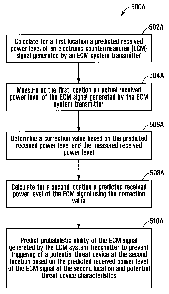
The method 500A begins at step 502A, in which a
predicted received power level of an ECM signal generated by
an ECM system transmitter is calculated for a first location
using a propagation and scenario model.
In step 504A, an actual received power level of
the ECM signal generated by the ECM system transmitter is
measured at the first location.
In step 506A, a correction value is determined
based on the predicted received power level and the measured
received power level.
In step 508A, a predicted received power level of
the ECM signal at a second location is calculated using the
propagation and scenario model and the correction value.
In step 510A, the probabilistic ability of the ECM
signal generated by the ECM system transmitter to prevent
triggering of a potential threat device at the second
location is predicted based on the predicted received power
level of the ECM signal at the second location and potential
threat device characteristics.
In some embodiments, the potential threat device
characteristics include an expected response of the
CA 02624433 2008-03-07
52925-4 34
potential threat device to the predicted received power
level of the ECM signal at the second location.
In some embodiments, there is an adaptive step
after step 506A to adjust parameters of the propagation and
scenario model until the predicted and measured received ECM
signal power levels substantially agree in order to enhance
the accuracy of the predicted received power level of the
ECM signal calculated in step 508A. This adaptive step may
include the use of genetic algorithms to refine the model
parameters in order to improve the model's predicted
results, as described herein.
In some embodiments, the device adaptively
modifies the internal model of the engagement to align the
prediction of the received power with the measured power,
and continuously refines the model and the estimates to
match ground-truth measurements, while accommodating
parameter uncertainties.
In some embodiments, a comparison of measured and
predicted power levels is used to generate a spectrum
mismatch cost function. If the mismatch cost function
exceeds a threshold value, a fault/anomaly may be indicated.
Model adaptation may involve adaptation of the nominal model
parameters that are judged by the user, or by the device, to
most likely be in error. The user may provide information
about which parameters are well known, and which are not.
The device may record the time history of various estimated
parameter values and discrepancies between predicted and
measured signal levels in order to derive information about
which parameters are well known, and which are not. Model
parameters that may have a strong impact on the accuracy of
CA 02624433 2008-03-07
52925-4 35
propagating and scenario models include, but are not limited
to antenna gains, heights, ranges, and transmitter power
levels. In general, the model may be adapted using user-
supplied information about uncertainties in the operating
environment.
Heuristic methods (e.g Genetic or Evolutionary
Algorithms) may be used to determine the optimal propagation
model parameters, i.e. the set of model parameters which
produce predicted pilot signal power levels that
substantially fit the measured levels. These methods
generally involve calculation of a "cost", based on a "cost
function". The "cost function" is defined as a mathematical
formula for calculating the cost. The "cost" is a numerical
quantity representing the agreement between predicted and
measured power levels. The cost depends on (i) the ground-
truth values of all scenario parameters, (ii) the predicted
values each of those model parameters which are subject to
optimization, and (iii) the radio frequency of the pilot
signals.
In some embodiments, two or more pilot signals
separated in frequency are used to simultaneously measure
multipath effects at different frequencies and the
propagation model is adapted until, for example, the RMS
error between the predicted and the measured power at all
frequencies is minimized or reduced to an acceptable level.
The acceptable RMS error is an implementation specific
detail.
Adaptation of the propagation model may be used to
remove discrepancies between measured and predicted power
levels arising from such factors as non-flat terrain (road
surface curvature), incorrect signal processing gain values
CA 02624433 2008-03-07
52925-4 36
used in the model (e.g. Tx, Rx antenna gains, Tx power,
etc.), incorrect range values used in the model, errors in
estimated road surface type, and/or incorrect antenna height
values used in the model.
Curvature of the road surface, i.e. hills or
valleys, can cause the vertical distance of potential
threats from the ECM system to differ between potential
threats that are the same horizontal distance from the ECM
system. Such curvatures may be the first parameter adapted
in the algorithm. If the road surface is curved, the height
of the ECM system, the height of the sensor, or the height
of the potential threat at a remote location could be
incorrectly represented in the model. However, in some
embodiments, the time history of model adaptations plus
known/expected/measured road curvature can be used to
eliminate or control the strength of this fact in the
adaptation algorithm.
In some embodiments, frequency diversity is used
to narrow the range of parameter value uncertainty. In
general, the more frequencies that are used, the more
uncertainty is removed. In some embodiments, a pattern of
signals that vary in frequency and amplitude (and possibly
also phase) is radiated such that it is possible to
determine one unique solution for the combination of
geometry of (a) the propagation environment, and (b)
material over which the signal propagates.
Figures 5B and 5BB illustrate a flowchart of a
more detailed example of a method that may be executed by
the device 106 shown in Figures 1 to 4. A detailed
description of the meaning of this flow chart is presented
below.
CA 02624433 2008-03-07
52925-4 37
The method includes a main computation loop 500B,
which may be executed repeatedly and indefinitely. The
method involves numerical calculations using the following
elements: (i) a model, (ii) a scenario model, (iii) a
protection range computational engine PRCE, and (iii) a
scenario parameter refinement engine (SPRE).
In some embodiments, the propagation model
comprises (a) a mathematical representation of all effects
deemed relevant to radio frequency propagation between
transmitters, receivers and scatterers of interest, and (b)
the algorithm used to solve for the parameters of interest
(i.e. the model outputs). The purpose of the propagation
model is to relate input parameter to radio frequency power
levels at a receiver antenna, for example at the sensor
antenna 108.
In some embodiments, the scenario model comprises
(a) nominal values and (b) variability values for all the
input parameters used by the propagation model and
protection range computational engine. The scenario model
also includes a parametric description of each possible
threat system of interest including nominal and variability
values for each parameter, whether or not an ECM has been
developed and/or deployed for a given threat. The purpose
of the scenario model is to provide inputs to the
propagation model and the PRCE. Some parameters in the
scenario model may be used only by the propagation model,
such as the geometry between receive and transmit antennas.
Some parameters of the scenario model may be used only by
the PRCE, such as algorithm-specific parameters, the
population size for statistical calculations (see step 519B
described below) and certain threat-specific parameters
CA 02624433 2008-03-07
52925-4 38
including receiver bandwidths and jamming-to-signal ratio
(JSR) to deny service between the threat transmitter and
threat receiver.
In some embodiments, the PRCE includes an
implementation of mathematical relationships, which relate
input parameters to estimates of ECM protection range for
each threat system. The purpose of the PRCE is to compute
various outputs related to the ECM protection range for each
threat.
In some embodiments, the SPRE includes a heuristic
algorithm based on Genetic Algorithms, as described
elsewhere in this document. The purpose of the SPRE is to
refine the value of selected scenario parameters based on
real-time measurements and inputs.
STEP 501B - MODEL CHANGE DETECTION:
The main computation loop 500B begins in a first
step 501B, in which a current scenario model is compared
with a scenario model used in a previous iteration of the
main computation loop 500B.
STEP 502B - DECISION/RESET WORST-CASE RECORDS:
In a second step 502B the algorithm implements a
decision: a determination is made whether the scenario model
has changed since the last iteration of the main computation
loop 500B.
STEP 503B - RESET WORST-CASE RECORDS:
In a third step 503B, proceeding from step 502B,
if there has been a change in the scenario model the
algorithm sets the worst-case protection range records for
CA 02624433 2008-03-07
52925-4 39
each threat to zero. The algorithm then proceeds to step
504B described below.
STEP 504B - RESET POPULATION AVERAGE CALCULATIONS:
In a fourth step 504B, proceeding from step 502B,
if there has been no change in the scenario model, the
output values calculated for a randomized population of
scenario parameter sets are reset, i.e. results of all
previous calculations performed by the main computation loop
500B are notionally set to zero. In some implementations,
results of previous calculations may be retained for later
use to (i) determine the effect of parameter changes on
computational results, and (ii) help accelerate and/or
refine the output of the main computational loop 500B.
STEP 505B - INITIAL ESTIMATE OF ECM POWER IN SENSOR:
In a fifth step 505B, the software calculates the
predicted ECM power level at a sensor antenna, such as the
sensor antenna 108 shown in Figures 1 to 4 and 21, based on
an initial estimate of propagation and scenario parameters.
STEP 506B - REFINEMENT OF NOMINAL MODEL PARAMETERS:
In a sixth step 506B, an algorithm is used to
refine the current estimate of (i) the nominal value and
(ii) expected variation range of selected parameters of the
scenario model. Examples of these parameters include
nominal ECM transmitter antenna height 113, nominal sensor
antenna height 112, and nominal transmitter-sensor antenna
range 110. This refinement is accomplished by the use of
measured pilot signal power levels and the use of heuristic
CA 02624433 2008-03-07
52925-4 40
methods such as Genetic or Evolutionary Algorithms, as
described herein.
STEP 507B - MODEL PARAMETER RANDOMIZATION:
In an seventh step 507B, each parameter value in
the scenario model is assigned a value randomly chosen from
within a specified range of variation relative to the
nominal value of the parameter. The variation range of each
parameter is preset as part of the scenario model, and
represents the accuracy with which each parameter is
believed to be known.
STEP 508B - ZERO-BEARING POWER ERROR:
In an eighth step 508B the ECM power at the sensor
antenna 108 is recomputed at the sensor bearing angle, i.e.
the bearing reference angle or zero bearing, using the
scenario parameter values set in step seven. The
discrepancy between the measured and predicted ECM powers at
the sensor antenna 108 is recorded as the zero-bearing power
error (ZBPE).
STEP 509B - BEARING INCREMENT:
With reference to Figure 21, in a ninth step 509B,
the bearing angle 564 at which the protection range for each
threat is to be calculated is incremented by a preset angle
565, producing a new bearing angle 566. The bearing angle
is the azimuth look angle from the ECM transmit antenna 104
in the direction that the ECM protection range will be
calculated. This angle is defined relative to the look
angle from the ECM transmit antenna 104 to the device sensor
antenna 108 bearing reference angle 560, i.e. the line of
sight 560 from the ECM transmit antenna 104 to the device
CA 02624433 2008-03-07
52925-4 41
sensor antenna 108 is defined to be the zero-bearing angle
560.
STEP 510B - RECALCULATION OF ECM POWER IN SENSOR:
In a tenth step 510B, the value of predicted ECM
power at the sensor antenna 108 is recalculated based on the
scenario parameters set in step 507B.
STEP 511B - ECM POWER IN THREAT RECEIVER CO-RANGE NOT CO-
HEIGHT:
In an eleventh step 511B, the ECM power is
calculated at a hypothetical threat receiver 122 which is
radially co-range but not co-height with the device sensor
antenna 108. The relevance of this computation in
determining the ECM protection range is based on the
untested hypothesis that the electromagnetic characteristics
of the local ground surface around the ECM antenna 104 is
invariant with bearing, i.e. propagation effects along the
zero-bearing line between the sensor antenna 108 and the ECM
antenna 104 apply at all bearings.
STEP 512B - TRIGGER POWER IN THREAT RECEIVER CO-RANGE NOT
CO-HEIGHT:
In a twelfth step 512B, the threat trigger power
is calculated in a hypothetical threat receiver 122 which is
co-range but not co-height with the device sensor antenna
108.
STEP 513B - REFINED ESTIMATE OF ECM POWER IN THREAT RECEIVER
CO-RANGE NOT CO-HEIGHT:
In a thirteenth step 513B, a refined estimate of
the ECM power in the threat receiver 122 is calculated using
CA 02624433 2008-03-07
52925-4 42
the zero bearing power error (ZBPE) calculated in step 508B
and the estimated ECM power in the threat receiver 122.
Transference of the ZBPE to the threat receiver power is
justified on the basis of the following untested hypotheses:
Hypothesis I: the sensor power discrepancy arises from
estimation errors which are common to the sensor antenna 108
and the threat receiver 122 at zero bearing, and Hypothesis
II: that this error is invariant with bearing.
Hypotheses I and II are predicted to be true if
the cause of the ZPBE is attributable to such factors as,
for example, misestimation of ECM transmitter power,
misestimation of installed ECM antenna gain, misestimation
of sensor antenna gain, and mismatch between the
polarization of ECM and sensor antennas. If one or both of
these hypotheses are not true, step 513B may introduce an
error in the calculated ECM protection range. Consequently,
in some embodiments, if information is available indicating
that Hypothesis I is invalid, step 513B may be omitted
altogether. If information is available indicating that
Hypothesis II is valid only for certain bearings, in some
embodiments, step 513B may be applied selectively, i.e. only
for those bearings at which Hypothesis II is known or
believed to be true.
STEP 514B - ECM PROTECTION STATE FOR THREAT CO-RANGE NOT CO-
HEIGHT:
In a fourteenth step 514B, the computed ECM and
threat trigger power in the threat receiver 122 is used to
calculate the estimated jamming-to-signal ratio (JSR) in the
threat receiver 122, with the threat receiver 122 at the
same radial range from the ECM transmit antenna 104 as the
sensor antenna 108, but at a different height. This is
CA 02624433 2008-03-07
52925-4 43
compared with the externally-supplied value of JSR to deny
service for each threat receiver-transmitter pair, to
determine if the ECM is capable of denying service between
the threat transmitter and receiver when (a) the threat
receiver 122 is radially co-range but not co-height with the
device sensor antenna 108, and (b) for the scenario
parameters set in step 507B.
STEP 515B - DETERMINE ECM EFFECTIVENESS TOGGLE RANGE (ETR):
In a fifteenth step 515B, the ECM protection range
for each threat is computed for the current scenario
parameter set(assigned in step 507B). This is accomplished
for each threat by re-computing the JSR in the threat
receiver at a plurality of hypothetical threat receiver 122
ranges radial from the ECM transmit antenna 104, in which
the only parameter of the scenario model varied is the range
of the threat receiver 122 from the ECM transmitter antenna
104. For each threat, the computed JSR value is compared
with the JSR to deny service, to determine whether the ECM
is able to deny service between the threat transmitter and
the threat receiver 122, at each of the hypothetical ranges.
The results of these calculations are used to determine the
range for each threat at which the ability of the ECM to
deny service between the threat transmitter and threat
receiver 122 changes from successful to unsuccessful, i.e.
to determine the so-called ECM effectiveness toggle range
(ETR). The ETR for each threat is defined as the computed
ECM protection range for (a) the current scenario parameter
set assigned in step 507B, and (b) the corresponding threat.
STEP 516B - ACCUMULATE AVERAGE ETR:
CA 02624433 2008-03-07
52925-4 44
In a sixteenth step 516B, the currently computed
ETR for each threat is recorded and used to accumulate an
average ETR over a plurality of scenario parameter sets.
Other measures of effectiveness are possible instead of
average ETR, including, for example, probability of service
denial vs. range, and probability of service denial vs.
range heuristically weighted by the statistically calculated
confidence of the probability (i.e. the weighting is
proposed, not derived).
In some embodiments, an average ERT is computed
separately for each threat. Additionally, the device 106
may record the predicted ECM spectrum in order to calculate
a number of statistical properties of a population of
predicted ECM spectra at the device sensor antenna 108,
including but not limited to the following:
(i) mean ECM power at each frequency;
(ii) standard deviation of ECM power at each
frequency;
(iii) ECM power in the absence of propagation
effects;
(iv) lowest predicted ECM power at each frequency;
and
(v) highest predicted ECM power at each frequency.
Examples of each of these curves are presented in
Figure 15, which is described in detail in a following
section.
STEP 517B - UPDATE WORST-CASE PROTECTION RANGE RECORDS:
CA 02624433 2008-03-07
52925-4 45
In an seventeenth step 517B, for each threat the
computed ETR is compared with the current record of worst-
case ETR. If the current value is less than the worst-case
ETR, the current value replaces the worst-case ERT for that
threat.
STEP 518B - DECISION/BEARING INCREMENT:
In a eighteenth step 518B, a determination is made
whether or not calculations described in steps 511B to 517B
have been applied to all bearings of interest. If they have
not, the algorithm returns to step 509B. If they have, the
algorithm proceeds to a nineteenth step 519B.
STEP 519B - DECISION/POPULATION COMPLETION:
In a nineteenth step 519B, a determination is made
whether or not the ETR has been calculated for a complete
population of scenario parameter sets, where the population
size is a preset parameter in the scenario model. Steps
507B to 518B inclusive comprise calculation of ETR value
versus bearing for each threat, for a single unique set of
scenario parameters which were randomly assigned in step
507B based on each parameter's nominal value and expected
variability. Because each randomized scenario parameter set
is unique, the ETR value versus bearing will generally vary
from one scenario parameter set to another and an average
set of ETR values versus bearing can be calculated from a
population of ETR values versus bearing, considering each
threat separately. If a complete population of ETR vs.
bearing has been generated for each threat, the algorithm
proceeds to step 501B. If the complete population of ETR
vs. bearing has not been generated for each threat, the
algorithm proceeds to step 507B in order to calculate ETR
CA 02624433 2008-03-07
52925-4 46
vs. bearing for another unique scenario parameter set, for
each threat.
By inclusion of step 507B, the probabilistic
effectiveness of the ECM system to prevent triggering of a
potential threat device at the second location is predicted
based on probabilistic characteristics of potential threat
devices because the scenario parameters used in prediction
(a) are randomized, and (b) include threat-specific
parameters such as for example threat transmit antenna gain,
threat receiver antenna gain, threat transmitter power,
threat receiver bandwidth, threat receive antenna
polarization, and threat transmit antenna polarization.
Implementation of a Heuristic Method for Parameter
Optimization
This section provides a description of the use of
a heuristic method for optimization of scenario model
parameters for use in predicting radio frequency signal
power levels at a plurality of locations.
Figure 5C is a flowchart of a heuristic method
550C for optimization of scenario model parameters for use
in predicting radio frequency signal power levels at a
plurality of locations.
With reference to Figure 5C, the method 550C
begins with a first step 551 in which an initial population
of candidate solutions is generated.
In a second step 552, the fitness of each
candidate in the population is evaluated against a fitness
function.
CA 02624433 2008-03-07
52925-4 47
In a third step 553, individuals are ranked
according to fitness.
In a fourth step 554, the best-performing
individuals are selected as individuals which will be used
to create the next generation.
In a fifth step 555, conditions are tested to
determine whether a stopping criterion or criteria have been
met. If they have been met, the method proceeds to a sixth
step 556 in which the search for an optimal solution is
terminated and the final solution has been found.
If the stopping criterion or criteria have not
been met in the fifth step 555, the method proceeds to a
seventh step 557 in which the next generation population of
candidate solutions is generated. The method then returns
to the second step 552.
In some embodiments, pilot signal power levels are
measured and compared with sets of predicted pilot signal
power levels, where each set of predicted pilot signal power
levels corresponds to an unique combination of candidate
scenario parameters. The purpose of the comparison is to
determine the ability of individual candidate scenario
parameter sets to predict the observed pilot signal power
levels. The fittest candidate parameter sets are those
which result in small discrepancies between predicted and
measured pilot signal power levels, considering all pilot
signals collectively. The fitness function is the
mathematical expression by which the candidate parameter
sets are ranked, considering all pilot signals collectively.
In some embodiments, one or more of the following
parameters may be selected for adaptation:
CA 02624433 2008-03-07
52925-4 48
(i) ECM transmitter antenna height;
(ii) Sensor antenna height;
(iii) Range between ECM and sensor antennas; and
(iv) ECM transmitter antenna gain.
The foregoing parameters are provided by way of
example only, and should not be construed as limiting.
Many choices are available for implementing the
following features of the heuristic method illustrated in
Figure 5C:
(a) the fitness function utilized in step 552;
(b) the algorithm for creating the next generation
candidate parameter set in step 557; and
(c) the stopping criteria utilized in step 555.
Specific choices for implementing the foregoing
features in some embodiments of the present invention are
described below.
Fitness Function:
In some embodiments, the fitness function
comprises a minimum ensemble error function according to:
(pMAAS PRED)2
y= !I
_, n
Where:
n = number of pilot signals;
CA 02624433 2008-03-07
52925-4 49
y = fitness value;
PMGAS = measured power of ith pilot signal; and
PRRED = predicted power of ith pilot signal
The formulation above is presented by way of
example only, since there is a nearly limitless range of
possibilities for the mathematical formulation of the
fitness function. For example, in some embodiments, the
contribution of each pilot signal frequency is weighted
according to the assessed value of the pilot signal
frequency in providing parameter set information.
In some embodiments, pilot signals at frequencies
for which a null is believed to be formed at or near the
device sensor antenna might be weighted differently than
others, because nulls typically only form for a narrow set
of parameter values. Under these conditions it might be
best to apply a relatively low weight to the term associated
with this pilot signal frequency in the ensemble cost
function. The anticipated effect is to avoid overly
penalising a parameter set which may be nearly correct, but
which makes a quantitatively large contribution to the
ensemble error value because a null occurs near the sensor.
Similarly, a relatively high weight could be applied for
terms associated with pilot signals at frequencies where a
relative maxima is believed to be formed at the device
sensor antenna.
Candidate parameter sets for which the fitness
function results in a value below a fitness threshold are
used to create the next generation of candidate parameter
sets.
CA 02624433 2008-03-07
52925-4 50
In some embodiments, the fitness threshold for
candidate survival is constant for all generations.
In some embodiments, as the overall fitness of
each generation increases, the threshold for contributing to
the next generation is adjusted to select only those
candidates which are the fittest relative to the overall
fitness of the population. This could potentially cause a
faster convergence of the solution by reducing the number of
sub-optimal candidates in each subsequent generation.
Algorithm For Creating Next Generation:
In some embodiments, one pair of parameter sets
which passed the fitness test (referred to as parent
parameter sets) may be used to create one new candidate
parameter set.
In some embodiments, the new value of each
parameter in the new parameter set is formed by taking the
algebraic average of the corresponding parameters in two
parent parameter sets. Successful parameter sets from the
previous generation may be randomly paired to form parent
parameter sets.
In some embodiments, the number of children
created is equal to the number required to replace the
candidate parameter sets which did not pass the fitness test
in the previous generation, less for example 10 percent of
the population of the previous generation.
In some embodiments, the next generation
population also has included in it a number of randomly
chosen parameter sets, where the parameter values are chosen
to lie within a parameter-specific and implementation-
CA 02624433 2008-03-07
52925-4 51
specific range of a parameter-specific and implementation-
specific nominal best-guess values.
The nominal value and parameter range from which
random candidates are generated may remain constant
throughout the optimization process.
In some embodiments, the number of randomly
generated parameter sets is for example 10 percent of the
population of the previous generation. The randomly chosen
parameter sets are included to help promote the discovery of
optimal solutions in parameter spaces which become poorly
sampled from one generation to the next, because of, for
example, possible clustering of parameter sets near
solutions which are only locally optimal.
The example algorithms described above for
creating a next-generation candidate parameter set are
illustrative only; there are a number of possible variations
which could be implemented. For example, the parent
parameter sets could be assigned according to fitness, e.g.
the parameter sets with the lowest score (highest fitness)
could be systematically paired with each other. Also, each
parent pair may not be limited to creating a single child
parameter set, but their productivity could be made
proportional to the combined fitness of the parent pair.
Alternatively, children could be created from single
survivors instead of from parent pairs, or there could be
several parents for each child parameter set.
Stopping Criteria:
In some embodiments, the stopping criteria
comprise the following:
CA 02624433 2008-03-07
52925-4 52
(i) Solution Convergence: the variability of
parameters in the candidate parameter sets has
become small enough that the candidates, or
candidates within a discrete number of groups,
are indistinguishable from each other;
(ii) Population Fitness Threshold: a preset fraction
of the population passes the fitness test; and
(iii) Timeout: a maximum allowed number of
generations has been executed.
The stopping criteria provided above are for exemplary
purposes only, and should not be construed as limiting.
Inclusion Of Threat Response:
In some embodiments, the potential threat device
characteristics include a predicted response of the
potential threat device to the predicted ECM system spectrum
at the second location.
Model Parameter Adaptation:
In some embodiments, there is an adaptive step
after step 505B to adjust parameters of the scenario model
until the predicted and measured power in pilot signals
(described below) and the ECM spectrum substantially agree
in order to enhance the accuracy of the predicted ECM system
spectrum as calculated in steps 510B, 511B, 512B and 515B.
This adaptive step may include the use of so-called
heuristic methods such as genetic or evolutionary algorithms
together with pilot signals to refine the value of selected
scenario parameters, in order to improve the model's
predictive power, as described herein. Heuristic methods
CA 02624433 2008-03-07
52925-4 53
are described in Goldberg, David E.; Genetic Algorithms in
Search, Optimization and Machine Learning; Addison-Wesley,
Boston, (c) 1989, ISBN 0201157675
The heuristic methods generally involve
optimization according to calculation of a "cost", based on
a "cost function". For the purposes of this description,
the "cost function" is defined as a mathematical formula
representing the agreement between predicted and measured
signal power levels. The cost depends on the following:
(i) the measured power and by extension the ground-
truth values of all scenario parameters
including transmitted power levels, and
(ii) predicted powers and by extension the estimated
values each of those model parameters which
are:
(a) used to predict power levels; and
(b) subject to optimization against the
cost.
In some embodiments, and for the purposes of this
explanation, the following points regarding the cost
function also apply:
(i) The cost is calculated from discrepancies
between measured and predicted pilot signal
characteristics such as for example power
levels,
(ii) it may be continuously applied in time, and
CA 02624433 2008-03-07
52925-4 54
(iii) it may use results of previous adaptation
activities to accelerate or refine ongoing
adaptation activities.
Additionally, adaptation activities may
accommodate the uncertainty of a parameter's optimal value
by setting:
(a) a search range for the parameter; and
(b) a confidence with which the final value is
believed to be known, respectively.
The parameters of the scenario model selected for
adaptation may be those that are judged by the user (a) to
most likely be in error and/or (b) to be known with the
lowest confidence. The user may provide information about
which parameters are well known, and which are not.
Scenario model parameters that may have a strong impact on
the accuracy of propagation and scenario calculations
include, but are not limited to Tx and Rx antenna gains,
relative heights, relative ranges, and transmitter power
levels.
Adaptation of the scenario model can also be used to
remove discrepancies between measured and predicted power
levels arising from such factors as non-flat terrain (road
surface curvature), incorrect signal processing gain values
used in the model (e.g. Tx, Rx antenna gains, Tx power,
etc.), incorrect range values used in the model, errors in
estimated road surface type, and/or incorrect antenna height
values used in the model.
Curvature of the road surface, i.e. hills or
valleys, can significantly affect propagation between the
CA 02624433 2008-03-07
52925-4 55
ECM transmit antenna 104 and a receiving antenna. This is
due to the following:
1: The effective height of potential threats
relative to the effective height of the ECM system is a
strong factor in determining multi-path interference between
direct and indirect (i.e. reflected) signals.
2: If a ray tracing approach is used to perform
multi-path calculations, the effective heights of both the
transmitter and receiver are determined by the location and
orientation of a tangent plane at the point of specular
reflection between the transmit and receive antennas.
3: The road surface curvature partially determines
the location and orientation of the tangent plane.
If the road surface is curved, the height of the
ECM system, the height of the sensor, or the height of the
potential threat at a remote location could be incorrectly
represented in the scenario model 630. However, in some
embodiments, the time history of model adaptations plus
known/predicted/measured road curvature could be used to
obviate or assist this aspect of the scenario model 630
adaptation algorithm.
Use Of Pilot Signals:
In some embodiments, so-called pilot signals are
used to determine the optimal value of selected parameters
in the scenario model. The definition of pilot signal
presented previously is repeated here for convenience: a
pilot signal is a signal transmitted by the ECM system 102,
and whose purpose is to provide information about the
characteristics of the communication channel through which
CA 02624433 2008-03-07
52925-4 56
the ECM signals propagate. There are two ways pilot signals
may be used:
(i) to assist heuristic methods in determining
optimal parameter values, and
(ii) to resolve selected parameter ambiguities.
When used with the heuristic methods for parameter
estimation, the pilot signals are used with a cost function
to adapt selected parameters in the scenario model 630 until
the cost is minimized or reduced to an acceptable level.
The cost, which drives the parameter adaptation, is
calculated from the difference between the predicted and the
measured pilot signal powers.
When used to resolve parameter ambiguities, the
measured pilot signal power levels are compared with
predicted values based on one or more possible parameter
values. An example of the use of two pilot signals is shown
in Figure 8 for a truck-mounted ECM jamming system 800 with
transmit antenna 801 and a truck-mounted sensing device 802
with receive antenna 803. The propagation model and power
measurements at multiple frequencies may reduce the range of
possible propagation geometry parameters (heights, range,
surface curvature, surface type), and in some cases may
provide a unique determination of the propagation geometry.
Examples are presented in following sections of
the use of pilot signals to:
(i) possibly resolve range ambiguities;
(ii) possibly resolve height ambiguities;
CA 02624433 2008-03-07
52925-4 57
(iii) possibly recognize and accommodate road
surface curvature; and
(iv) possibly identify unrecognized road
conditions which could decrease the
confidence of the ECM protection range
prediction.
In some embodiments, the pilot signals may be
present and used in the one or more of the following ways:
(i) several pilot signals are present and used
simultaneously; and
(ii) a single pilot signal is present and used whose
frequency is varied continuously or discretely
in time.
Both implementations are equivalent to using the
frequency diversity of pilot signals to (a) narrow the range
of uncertainty of the final estimated value of selected
scenario parameters in the scenario model 630, and (b)
improve the confidence of the final estimated values.
In general, as more frequency diversity is used
the uncertainty in the final estimated values of adapted
scenario parameters becomes less, and the confidence becomes
greater. The case of a single pilot signal with variable
frequency is discussed in greater detail in a following
section with reference to Figures 17A - 20D.
In some embodiments, pilot signals are radiated in
an implementation- and scenario-specific pattern in
frequency and amplitude (and possibly also phase) in order
to improve the accuracy and confidence of the final
CA 02624433 2008-03-07
52925-4 58
parameter values, including for example (a) the geometry of
the propagation environment, and (b) material over which the
signal propagates. For example, the set of pilot signal
frequencies may be chosen and adjusted in order to confirm
the location of predicted multipath nulls and/or power peaks
at the device sensor antenna 108, to test specific
hypotheses regarding transmitter-receiver range, transmitter
antenna height, and sensor antenna height, as well as to
test hypotheses regarding the variability of selected
scenario model parameters a discussed below in association
with Figure 16A and Figure 16B.
The frequency, amplitude or phase pattern may be
(a) pre-scripted, i.e. determined a priori for use under
certain recognizable field conditions, or (b) adaptive in
time, for example the frequency of one or more pilot signals
may be varied in time in order to probe the characteristics
of the communication channel between the ECM transmit
antenna 104 and the sensor antenna 108. An example is
presented in the discussion of Figure 10 above to justify
pre-scripted or adaptive pilot signal frequency selection.
A more detailed discussion of pilot signal frequency
adaptation is presented below.
Pilot Signal Frequency Adaptation:
Pilot signals at a plurality of frequencies can be
used with heuristic methods to find model parameters that
more closely match the measured and predicted pilot signal
power levels.
In some embodiments, pilot signal selection is
adaptive. An example of adaptive pilot signal selection is
illustrated in Figures 13A and 13B for a scenario in which
CA 02624433 2008-03-07
Y :
52925-4 59
an ECM transmit antenna 1302 is located on a first convoy
truck 1300 and a device sensor antenna 1306 is located on a
second convoy truck 1304 physically remote from the first
convoy truck. Figure 13A illustrates the predicted power at
the device sensor antenna 1306 versus frequency for an
example set of six pilot signals 901-906 at equally spaced
frequencies that might be initially selected. Figure 13B
illustrates the adaptive adjustment of the pilot signals
shown in Figure 13A, i.e. the adjustment of the center
frequencies of the six pilot signals 901-906 and the
addition of three new pilot signals 907-909.
In addition to the pilot signals 901-906, Figure
13B also illustrates the predicted received ECM spectral
powers 910-926 for nine different parameter sets for the
scenario model. The scenario model parameter set for which
the measured pilot signal power levels 950 - 966 most
closely match the predicted pilot signal power levels 901 -
909 represents the optimal set of model parameters for
predicting the ECM protection range.
In the example of Figure 13B the calculated ECM
spectrum 910 most accurately predicts the measured powers
for the nine pilot signals 901-909. The other predicted ECM
spectra 912-926 include some error in one or more of the
model parameters, and do not as accurately predict the
measured pilot signal powers 950 - 966 for each of the pilot
signals 901-909. Specifically, calculated power spectra
912, 914, 916 and 918 are the result of an error in the
range parameter of -3m, -1.5 m, +1.5 m and +3m from the true
range, respectively, calculated power spectra 920 and 924
are the result of an error in the sensor height parameter of
0.1m and +0.lm, respectively, and calculated ECM spectra 922
CA 02624433 2008-03-07
52925-4 60
and 926 are the result of an error in the ECM system height
parameter of +0.2m and -0.2m, respectively.
As noted above, Figure 13B illustrates an example
of how the selection of the pilot signals might be
adaptively adjusted, i.e., how pilot signal frequencies may
be changed and/or new pilot signals may be added, and the
power levels monitored, in order to confirm the multipath
solution by refining the model parameter selection. In some
embodiments, adaptively adjusting the pilot signal selection
may involve (a) direct, (b) indirect or (c) no communication
between the device sensor and the unit that injects the
pilot signals into the ECM antenna(s), in order to
synchronize the frequencies of the transmitted pilot signals
with the pilot signal frequencies predicted by the device
106.
Examples of direct communication include infrared,
acoustic, vibration, or radio frequency communications
links.
An example of indirect communication link is the
use of an external timing reference such as is provided by
the Global Positioning System.
An example in which said synchronization is
achieved with no communication between the sensor device and
the unit that injects the pilot signals might be when a
pilot signal acquisition capability is included in the
implementation of the sensor device, i.e. the device scans
certain frequency bands to acquire a preset number of pilot
signals, possibly identified from background signals and
made resistant to hostile jamming by frequency or phase
modulation.
CA 02624433 2008-03-07
52925-4 61
In Figure 13B, the pilot signals 901-909 have been
arranged in the frequency spectrum in order to accommodate
potentially conflicting requirements such as for example (i)
maximize the signal-to-noise ratio of the pilot signal and
(ii) distinguish the power level predictions of various
candidate scenario parameter sets.
In the example of Figure 13B, pilot signal
frequencies have been selected such that (a) more pilot
signals are located in a region 931 where the predicted
power levels 901 - 903 are substantially different from one
another, (b) more pilot signals are located in regions 932
and 934 where a relative null is predicted, and (c) fewer
pilot signals are located in a region 933 where the
predicted power 906 is relatively invariant with frequency.
For example, only a single pilot signal 906 is used to
define the region 933, whereas three pilot signals 907-909
are used to define the region 934 in which many of the
predicted spectra 910-926 have propagation "nulls". With
more pilot signals, there are more points to fit the
predicted spectra to in order to determine a more accurate
set of model parameters.
The results shown in Figures 13A and 13B are
provided by way of example only, and should not be construed
as limiting. It should be appreciated that the variation in
the predicted ECM spectrum due to parameter variation is
dependent on the specific propagation and scenario model
used, and measured power levels to which the predicted power
levels depend on various and sundry field conditions.
Results different from that shown in Figures 13A and 13B may
be obtained under the same or different circumstances.
CA 02624433 2008-03-07
52925-4 62
Pilot Signals Used To Resolve Range Ambiguity:
In Figure 8, a graph is presented comprising two
curves of predicted received signal power at a sensing
device antenna 803 vs. range from the ECM transmit antenna
801 to the sensing device 802. The curves 804 and 804 are
generated using a propagation model which uses parameters
provided by a scenario model. The first curve 804
represents received power predicted for a pilot signal
frequency of 200 MHz. The second curve 806 represents
received power predicted for a pilot signal frequency of
1800 MHz.
To illustrate the resolution of a range ambiguity,
consider first the received power curve 806 for 1800 MHz in
Figure 8. The received power at a first range 812 is
indicated at 816. According to the propagation model used
to create the 1800 MHz curve 806, the received power 816 is
also observed at a second range 814.
The prediction of an identical power level 816 at
1800 MHz at two different ranges 812 and 814 represents a
range ambiguity, i.e. at 1800 MHz there are two ranges 812
and 814 which result in a single value of predicted power
816. To resolve this ambiguity, consider the received power
curve 804 for 200 MHz.
The received power at the first range 812
predicted for 200 MHz is indicated at 818, and at the second
range is indicated at 820. The power levels 818 and 820 are
not equal. If the predicted powers at 1800 MHz and 200 MHz
are considered as a data pair valid for a single range
between the transmit antenna 801 and the receive antenna
803, then the prediction pair 816 and 818 at the first range
CA 02624433 2008-03-07
52925-4 63
812 is distinct from the prediction pair 816 and 820 at the
second range 814. Because the prediction pairs are distinct
in range, the range ambiguity in the predicted power 816 at
1800 MHz is resolved.
In the example presented in Figure 8, measured
pilot signal power at 200 MHz 822 and at 1800 MHz 824 most
closely match the prediction pair 816 and 820 at the second
range 814, revealing that the second range 814 is the best
estimate of the true range between the transmit antenna 801
and the receive antenna 803.
Pilot Signals Used To Resolve Height Ambiguity:
Pilot signals at different frequencies may be
similarly used to resolve ambiguities in receiver or
transmitter heights. In a manner analogous to that
described for range ambiguities, it is possible that two
height values for a transmit or receive antenna may produce
the same power level at a receive antenna at a single pilot
signal frequency. As an example of this, consider Figures
10A and 10B.
Figures l0A is a graph 1002 of power received at a
device sensor antenna versus range for pilot signals at
three frequencies and two candidate heights of an ECM
transmit antenna. An enlargement 1003 of a portion of the
graph 1002 is presented in Figure l0B for clarity. The
graphed lines presented in graphs 1002 and 1003 were
calculated using a propagation model with parameter set from
a scenario model in which the device sensor antenna height
is 1.70 m. Curves representing calculated power at the
device sensor antenna vs. range are presented in graphs 1002
and 1003 for the following cases:
CA 02624433 2008-03-07
52925-4 64
1004 - 200 MHz pilot signal, transmitter antenna
height of 2.50 m;
1006 - 200 MHz pilot signal, transmitter antenna
height of 1.70 m;
1008 - 1800 MHz pilot signal, transmitter antenna
height of 2.50 m;
1010 - 1800 MHz pilot signal, transmitter antenna
height of 1.70 m;
1012 - 2000 MHz pilot signal, transmitter antenna
height of 2.50 m; and
1014 - 2000 MHz pilot signal, transmitter antenna
height of 1.70 m.
In the example of Figures 10A and 10B, the power
of the 1800 MHz pilot signal at the device sensor antenna at
42.7 m range 1016 is predicted to be -66.5 dBm, generally
indicated at 1018, for both candidate transmit antenna
heights, i.e. as indicated by the 1800 MHz 2.50 m curve 1008
and the 1800 MHz 1.70 m curve 1010. Because a single power
measurement value 1018 is predicted at 1800 MHz for the two
different transmit antenna heights, the predicted power
level 1018 does not unambiguously determine the height of
the transmitter antenna.
This ambiguity can be resolved if a second pilot
signal is used. To illustrate this ambiguity resolution,
consider the predicted power in the device sensor antenna at
2000 MHz. The predicted received power 1014 for a
transmitter antenna height of 1.70 m at a range of 42.7 m is
-73 dBm 1020. The predicted received power 1012 for a
CA 02624433 2008-03-07
52925-4 65
transmitter antenna height of 1.70 m is -64 dBm 1022. If
the predicted powers at 1800 MHz and 2000 MHz are considered
as a prediction pair for a sensor range of 42.7 m, then
predicted powers for the two Tx height cases 2.50 m and 1.70
m are distinct and the ambiguity is resolved. In the
example presented in Figures 10A and 10B, measured pilot
signal power at 1800 MHz 1024 (-66.5 dBm) and at 2000 MHz
1026 (-73 dBm) most closely match the prediction pair 1018
(-66.5 dBm) and 1020 (-73 dBm) at a range of 42.7 m,
revealing that a 1.70 m height is the best estimate of the
true ECM transmitter height 113.
The example presented in Figures 10A and 10B
illustrates a secondary point regarding the selection of
pilot signal frequency: that some choices of pilot signal
frequency may be better than others for (for example) the
purpose of resolving parameter ambiguities. Consider the
case in which the frequency of the second pilot signal is
chosen to be 200 MHz instead of 2000 MHz. At 42.7 m range
1016 the predicted signal power for an ECM transmitter
antenna height of 2.50 m is -50.8 dBm 1030 and the predicted
power for an ECM transmitter antenna height of 1.70 m is -
53.5 dBm 1028. The difference between the predicted power
for the 2.50 m case 1028 and the 1.70 m case 1030 is 2.7 dB.
Considering the case presented above where the second pilot
signal frequency is 2000 MHz, the difference between the
predicted power for the 2.50 m case 1020 (-73 dBm) and the
1.70 m case 1022 (-64 dBm) is 9 dB.
If the accuracy of the measured pilot signal
powers is of the order of the power difference predicted for
the two heights (e.g. +-2 dBm), then in the example of
Figures 10A and 10B the use of a second pilot signal at 200
CA 02624433 2008-03-07
52925-4 66
MHz may be less suitable than a pilot signal at 2000 MHz,
and may be unsuitable for resolving the ambiguity
altogether. This effect may also be seen if pilot signal
frequencies are whole number multiples of each other, e.g.
parameter ambiguities for a pilot signal at 1800 MHz may be
identical to some or all of those for pilot signal at 900
MHz. For this reason, pre-scripted pilot signal frequencies
and amplitudes, and adaptive selection of pilot signal
frequencies and amplitudes, may be implemented in some
embodiments.
Effect Of Road Surface Curvature:
Under certain conditions it is possible to use the
measured power of pilot signals at different frequencies to
detect and/or estimate road surface curvature. Provided
that propagation conditions exist in which a ray tracing
propagation model is valid, and provided that a model of
road curvature applies to the field conditions (e.g. a
singly curved concave or convex surface) the effect of road
curvature is to alter the effective height of the ECM
transmitter antenna and/or the effective height of the
device sensor antenna.
Referring to Figures 11A and 11B, consider two
hypothetical cases: (i) a convex road surface 1180, as
illustrated in Figure 11A, and a concave road surface 1190,
as illustrated in Figure 11B. The physical height of a
transmit antenna 1100 above the curved road surface 1102 is
indicated at 1104, and the physical height for a receiver
antenna 1106 is indicated at 1108.
According to a ray tracing propagation model, the
interaction of the direct and reflected or multi-path
CA 02624433 2008-03-07
52925-4 67
signals over a curved surface can be represented by
transforming the curved surface propagation problem into a
flat plane propagation problem. This can be accomplished by
applying Snell's Law (i.e. equal angles of incidence 1110
and reflection 1112 at the ray reflection point 1114) at a
plane 1116 which is tangent to the curved road surface 1102
point of reflection 1112. The transmitter antenna 1100 is
at an effective height 1118 above the tangent plane, and the
receiver antenna 1106 is at an effective height of 1120
above the tangent plane. In these cases, the effect of road
curvature may be determined by using multiple pilot signals
in the manner already described for height ambiguities,
referring to Figures 10A and 10B and the discussion related
to Figures 10A and 10B.
The use of Snell's Law to transform a curved
surface propagation problem into a flat plane propagation
problem is described in Hirsch, H and Grove, C.; Practical
Simulation of Radar Antennas and Radomes, Artech House, 685
Canton St., Norwood, MA USA 02062, 1987, ISBN 0-89006-237-4,
p. 189.
Detection Of Unrecognized Propagation Conditions:
Under certain conditions it may not be possible to
create a scenario model which matches the current operating
conditions, i.e. there may be no set of scenario parameters
which match the operating conditions sufficiently well to
produce an adequately confident estimate of ECM protection
range. Such conditions could include, but may not be
limited to, any or all of the following:
(i) an unrecognizably irregular road surface, i.e.
a road surface which is topologically distinct
CA 02624433 2008-03-07
52925-4 68
from the class of road surfaces which can be
represented by parameter sets in the scenario
model, for example a multiply curved surface
which may not be adequately represented by a
singly curved surface or a flat surface;
(ii) the presence of spurious transmitters in the
environment;
(iii) the presence of spurious scatterers in the
environment; and
(iv) defects or alterations in ECM- or device-
related equipment.
It may be possible for a sensor device in accordance
with an embodiment of the present invention to detect, and
in some cases identify, the existence of such conditions and
take remedial action, for example, issue a warning to the
user (s) .
As an illustration of this, consider Figures 12A,
12B and 12C. Figures 12B and 12C include the following
principal features:
1. A vehicle 1200 equipped with an ECM system
102 and ECM transmit antenna 1202.
2. A vehicle 1204 equipped with the device
106 and device sensor antenna 1206.
3. An irregular road surface 1208 comprising
a series of road surface segments 1210-
1224 whose shape in each case is
CA 02624433 2008-03-07
52925-4 69
represented by a segment of the
circumference of a circle having a
specific radius 1226-1240 respectively.
A single direct propagation 1242 path is shown
separately for clarity in Figure 12B, together with two
hypothetical indirect propagation paths 1244 and 1246
corresponding to specular reflection points 1248 and 1250,
respectively.
A hypothetical graph is presented in Figure 12A
representing pilot signal power in the device receiver
antenna 1206 versus range, comprising several curves:
(i) predicted pilot signal power 1254 for a pilot
signal at a first frequency, assuming a flat
road surface;
(ii) predicted pilot signal power 1256 for a pilot
signal at a second frequency, assuming a flat
road surface;
(iii) predicted pilot signal power 1258 for a pilot
signal at a third frequency, assuming a flat
road surface;
(iv) actual pilot signal power 1260 for a pilot
signal at a first frequency;
(v) actual pilot signal power 1262 for a pilot
signal at a second frequency; and
(vi) actual pilot signal power 1264 for a pilot
signal at a third frequency.
CA 02624433 2008-03-07
52925-4 70
Consider an example test range 1266. The predicted
pilot signal power levels at the three pilot signal
frequencies are 1268, 1270 and 1272 respectively, based on
curves 1254, 1256 and 1258, respectively.
The pilot signal power levels observed at the test
range 1266 are 1274, 1276 and 1278 respectively based on the
actual pilot signal power curves 1260, 1262 and 1264
respectively. There are discrepancies between the measured
and predicted pilot signal power levels at the test range
1266.
For the purposes of this example, the pilot signal
power measurement error is assumed to be smaller than the
discrepancies between the predicted and measured pilot
signal power levels. Under these conditions, the device 104
may indicate to an operator by a suitable signal that
unrecognized conditions have been sensed, i.e. the
characteristics of the discrepancies between the predicted
and measured pilot signals are sufficient to indicate a high
probability of unrecognized operating conditions, which in
the example of Figures 12A, 12B and 12C arises from an
irregular road surface, and consequently the confidence of
the ECM protection range prediction is reduced.
Following the example of Figures 12A, 12B and 12C
further, if a scenario model can be used which allows for
two (or more) specular reflection points, it may be possible
for a sensor device in accordance with an embodiment of the
present invention to deduce the correct scenario model for
the operating conditions, increasing the confidence of the
ECM protection range prediction.
ECM Fault/Anomaly Detection:
CA 02624433 2008-03-07
52925-4 71
In some embodiments, a comparison of measured and
predicted ECM spectra is used to generate a spectrum
mismatch cost. The mismatch cost may indicate excessive or
insufficient ECM power relative to the expected ECM power as
established for example by (a) specifications published by
the manufacturer of the ECM equipment and/or (b) the
believed performance of the scenario parameter estimation
calculations and/or (c) unexpected irregularities in the
propagation environment such as for example occlusion of the
ECM transmit antenna from the sensor antenna by another
vehicle or vehicles, the presence or sudden appearance of
hill(s), ditch(es), vehicles, or man-made object(s) as the
ECM vehicle moves through terrain.
If the mismatch cost function exceeds a threshold
value, a fault and/or anomaly may be indicated. A fault is
defined as a state in which the measured ECM spectral power
is significantly below the predicted minimum value, for
example, a state in which the predicted ECM radio frequency
power over a spectral window is below the predicted value by
a margin which may be user-defined or calculated by the
sensor device. The definition of an anomaly is identical to
that of a fault except the measured power significantly
exceeds the predicted maximum value over a spectral window,
by a similarly defined margin. This is illustrated
qualitatively in Figure 9.
Figure 9 is a graph 9900 of radio frequency power
vs. radio frequency on which several graphed lines are
presented. These lines include the following:
(a) measured power 9902 at a device antenna;
CA 02624433 2008-03-07
52925-4 72
(b) predicted power 9904 at the device antenna as
calculated by the device;
(c) the maximum power 9906 predicted at the device
antenna as calculated by the device based on
the predicted variability 9908 of the predicted
power 9904 where the variability 9908 is
derived for example from the ECM manufacturer's
specifications and the calculated cumulative
effects of various and sundry uncertainties in
the scenario model; and
(d) the minimum power 9910 at the device antenna
defined similarly as the maximum power 9906.
In the example of Figure 9, the following fault
and anomaly regions are evident:
(i) two regions of anomaly 9912 and 9916, in which
the measured ECM power is greater than the
predicted ECM power by a margin greater than,
for example, half the calculated power
variability 9908; and
(ii) one region of fault 9914 in which the measured
ECM power is less than the predicted ECM power
by a margin greater than for example half the
calculated power variability 9908.
In practice, the thresholds for maximum and
minimum predicted ECM power may be statistically derived
from one or more populations of predicted ECM power at the
device sensor antenna, calculated from one or more
populations of scenario parameter sets. These scenario
parameter sets may be generated as described previously in
CA 02624433 2008-03-07
52925-4 73
Step 507B of the method illustrated in Figure 5B. The
maximum and minimum thresholds, as well as other curves
derived from the population(s), may be calculated as
described above with reference to Step 516B of the method
illustrated in Figure 5BB.
An example of the maximum and minimum thresholds
derived from a population of scenario parameter sets is
presented in Figure 15. Figure 15 shows an example plot of
the variation of a measured ECM power 950 and several
calculated ECM power levels as a function of frequency. The
calculated power levels include the following:
(i) an ideal received power (no propagation loss)
962 at each frequency;
(ii) a best-case received power 954 at each
frequency;
(iii) a worst-case received power 956 at each
frequency;
(iv) a mean plus standard deviation received power
958 at each frequency;
(v) a mean minus standard deviation predicted power
960 at each frequency; and
(vi) a mean predicted power 952 at each frequency.
In Figure 15, the calculated power levels 952-962
are derived from a population of 26 predictions of the ECM
spectrum at the device sensor antenna 108 in accordance with
an embodiment of the present invention. For example,
results such as those in Figure 15 may be calculated after N
number of repetitions of the method illustrated in Figures
CA 02624433 2008-03-07
52925-4 74
5B and 5BB, where the best-case and worst-case ECM spectral
powers are updated in Step 516B for each scenario parameter
set. Statistical information on the measured and calculated
ECM power levels, such as the results plotted in Figure 15
may be more valuable to a community of supporting technical
people rather than to the in situ end-users of a sensing
device. For example, the information could be used in any
or all of the following ways:
(i) Forensic Evidence: recorded continuously as
forensic evidence to be used after an attack;
(ii) Trouble Shooting: used to either confirm the
health of a given device unit, or to diagnose
faults;
(iii) Trials Support: as a diagnostic tool in
planning and executing proving trials to
demonstrate operational readiness;
(iv) Product Development and Enhancement: during
software and hardware product development; and
(v) Marketing: to provide technical credibility
that the device operates.
Parameter Uncertainty Estimation:
In some embodiments, a sensing device estimates
not only the value of certain parameters in a scenario
model, but also (a) assesses the suitability of the
variation range (i.e. the uncertainty) assigned to the
parameter(s) in the scenario model and (b) corrects the
variation range if it is assessed to be unsuitable. A
CA 02624433 2008-03-07
52925-4 75
description of an example method by which this could be
accomplished is presented below.
In order to accommodate uncertainty in various
scenario parameters, the predicted power levels calculated
by a sensing device may be average values based on a
population of unique scenario model parameter sets, for
example, ECM antenna height, sensor antenna height, ECM-
sensor range, and ECM antenna gain. Each member of the
population comprises a unique combination of values for
these scenario parameters, created by a random assignment of
scenario parameters based on the scenario model including
(i) a nominal value for each parameter, and (ii) the
variability assigned to each parameter. For example, the
randomization of parameter values may be performed in a step
similar to step 507B in Figure 5B, and the average ECM power
may be calculated in a step similar to step 516B in Figure
5BB.
If the true scenario parameters produce a
propagation null in the measured signal power at the device
sensor antenna for a given pilot signal frequency there can
be a large discrepancy between the mean predicted pilot
signal power level and the measured pilot signal power
level. This could potentially occur because only a specific
and narrow range of parameters produces a relative
propagation null, so most of the scenario parameter sets
from which the mean power level is derived will not produce
a null at the device sensor antenna. The effect of
averaging over many possible scenario parameter sets results
in an average predicted pilot signal power which is
significantly higher than the measured value. If the
measured power indicates that the device sensor antenna is
CA 02624433 2008-03-07
52925-4 76
in or near a propagation null, then a relatively large
discrepancy between the measured and mean predicted pilot
signal power levels may suggest that the variability of one
or more scenario model parameters is excessively large.
Under certain circumstances it may be possible to
reduce the discrepancy by adjusting the variability of
various scenario model parameters without changing the
nominal value of said parameters.
By this method it may be possible for the device
to use the heuristic methods referenced previously or other
methods to adaptively estimate the variability (uncertainty)
of various scenario model parameters as well as the best
estimate of their nominal value, particularly if pilot
signal frequency is adapted, i.e. varied in a controlled
manner to, for example, attempt to observe a propagation
null at the device sensor antenna.
Figure 16A is an example plot of a measured ECM
power spectrum 964 and an average calculated ECM power
spectrum 966, each graphed as a function of frequency. The
ECM spectrum includes pilot signals at three frequencies
971, 972 and 973. The measured ECM power spectrum 964 has a
propagation null at the frequency 972 of one of the pilot
signals. The calculated ECM power spectrum 966 in Figure
16A is the average result for a sensor range uncertainty of
+/- 3 meters, with a uniform probability density function.
In general there is a discrepancy between the
average calculated pilot signal powers 978, 980, 982 978 and
the measured pilot signal powers 984, 986, 988 respectively.
Consider the discrepancy 976 for the pilot signal frequency
972 for which, in this example, a propagation null occurs
CA 02624433 2008-03-07
52925-4 77
for the given set of scenario parameters. The discrepancy
976 (23 dB) between measured pilot signal power 986 (-58
dBm) and average pilot signal power 980 (-35 dBm) is large
relative to that at the other pilot signal frequencies 971
and 973 (23 dB discrepancy compared with approximately 2 dB
and 2 dB discrepancies respectively) because only narrow
ranges of scenario model parameters produce power nulls.
For this reason, the calculated average power levels may
exhibit relative power minima 990 near nulls which exist for
specific parameter sets but will not show well-formed power
nulls if they are calculated from populations of candidate
model parameter sets in which parameters vary across
relatively broad value ranges.
The difference 976 between the measured 986 and
calculated mean 980 pilot signal power levels may be reduced
or eliminated by iteratively adjusting (a) nominal model
parameter values and (b) the uncertainty associated with
each parameter that is used to generate the population on
which the average predicted power is based. By minimizing
the difference between measured and average predicted power
levels for each pilot signal, an estimate is obtained for
each model parameter as well as the uncertainty associated
with the estimate.
Figure 16B shows an example plot of a measured ECM
power level 965 and a calculated ECM power level 967 in
which the discrepancy 992 at the pilot signal frequency 972
has been reduced by (i) adjusting the value of the sensor
range parameter in the scenario model to match the true
range value, and (ii) reducing the uncertainty associated
with this parameter from +-3 m to +-0 m (i.e. no
uncertainty).
CA 02624433 2008-03-07
52925-4 78
Pilot Signal Frequency Variation:
In some implementations, only a single pilot
signal is used at any moment, i.e., an ECM system generates
only a single pilot signal that a sensing device in
accordance with an embodiment of the present invention can
use to characterize the propagation channel and refine the
propagation and scenario model parameters.
In some embodiments, the centre frequency of the
single pilot signal is varied in time either in discrete
steps or continuously. The purpose of this temporal
frequency variation is to (a) refine the set of propagation
model parameters which result in a model output that
substantially matches the measurement observations at all
frequencies, and (b) estimate the uncertainty in the best-
estimate of each parameter based on the discrepancies
between the measured and best-estimate predicted power.
Variation of the pilot signal frequency produces a
profile of pilot signal power vs. frequency. Assuming the
reflecting surface between the transmitter and receiver is
flat, or locally flat at the single specular reflection
point, this profile may be assumed to be unique for the
physical attributes of the propagation channel, i.e., it is
unique for a single combination of transmitter height,
receiver height, transmitter-receiver range and surface
type. For proper device operation the power vs. frequency
profile need only be unique within the range of admissible
scenario model parameter values. This range of values is
application specific, e.g. if the observed pilot signal
power corresponds to sensor heights of for example 1 m, 25
m, 33 m, and 38 m and if, for example, sensor heights above
2 m are computationally inadmissible, then the measured
CA 02624433 2008-03-07
52925-4 79
pilot signal power effectively corresponds to a unique
sensor height.
Figures 17A and 17B are example graphs showing the
power profile at a device sensor antenna at five arbitrarily
chosen frequencies as a function of transmitter-receiver
range for a fixed transmitter antenna height of 1.7 m and a
fixed device sensor antenna height of 1.7 m. Referring to
Figure 17A, the received power curves 1780, 1781, 1782,
1783, and 1784 correspond to pilot frequencies of 150 MHz,
300 MHz, 500 MHz, 900 MHz and 1800 MHz, respectively.
Figure 17B comprises an example plot of received powers 1785
and 1786 as a function of pilot signal frequency for two
ranges R1=9 m and R2 = 15m respectively. Differences
between the two received power curves 1785 and 1786 indicate
that the measurements were taken at different ranges. If
the received power curves 1785 and 1786 are unique, i.e. no
other combination of model parameters yields the same
received power vs. pilot frequency result, and the bounds on
the range parameter are set to include R1 and R2, then the
received power vs. frequency results can be used to uniquely
define a single set of propagation model parameters such
that the model output matches the measurement observations
at each pilot frequency.
A similar example for transmitter antenna height
variation is presented in Figures 18A and 18B. Figure 18A
comprises received power curves 1890, 1891, 1892, 1893 and
1894 as a function of transmit antenna height for pilot
signal frequencies corresponding to 150 MHz,300 MHz, 500
MHz, 900 MHz and 1800 MHz, respectively. Figure 18B is an
example plot of received power 1892 and 1893 vs. pilot
signal frequency at two transmit antenna heights
CA 02624433 2008-03-07
52925-4 80
corresponding to 2.2 m and 1.7 m, respectively, taken from
the received power curves 1890, 1891, 1892, 1893 and 1894 of
Figure 18A. Because the curves 1892 and 1893 are distinct,
they represent distinct observation sets for the two cases
of transmitter antenna height.
If the admissible values of transmitter antenna
height are suitably constrained in the scenario model
according to a specific implementation of the device, then
as described above for variation of transmitter-receiver
range in Figure 17A and Figure 17B the observations are
unique as well as distinct with respect to transmitter
antenna height.
Figures 19A and 19B depict similar plots for
variations in receiver antenna height. In Figure 19A,
received powers 1994, 1995, 1996, 1997 and 1998 are plotted
as a function of receiver antenna height for pilot signal
frequencies of 150 MHz, 300 MHz, 500 MHz, 900 MHz and 1800
MHz, respectively. The received powers 1999 and 2000 for
two values of receiver antenna height corresponding to 2.2 m
and 1.7 m as a function of pilot signal frequency are
plotted in Figure 18B. Because the curves 1999 and 2000 are
distinct, they represent distinct observation sets for the
two cases of receiver antenna height.
If the admissible values of receiver height are
suitably constrained in the scenario model according to a
specific implementation of the device, then as described
above for variation of transmitter-receiver range in Figure
17A and Figure 17B and transmitter height in Figure 18A and
Figure 18B, the observations are unique and distinct with
respect to receiver antenna height.
CA 02624433 2008-03-07
52925-4 81
In Figures 17B, 18B and 19B, the graphs of
received power vs. pilot signal frequency are equally
graphs of power vs. time as the single pilot frequency is
scanned from, for example, low frequency to high. The
variation of the centre frequency of a single pilot signal
is represented graphically in Figures 20A to 20D for the
three cases illustrated in Figures 17A, 17B, 18A, 18B, 19A
and 19B, which, results in a distinct pattern of received
pilot signal power level vs. frequency/time. As noted above
for Figures 17B, 18B and 19B, if the admissible values of
the respective scenario parameters are suitably constrained
in the scenario model according to a specific implementation
of the device, then the graphs of power vs. time are unique
and distinct and so uniquely determine scenario parameters.
Figure 20A illustrates the step-wise variation of
pilot signal frequency 1002 as a function of time through
the five pilot signal frequencies: 150 MHz, 300 MHz, 500
MHz, 900 MHz and 1800 MHz. Figure 20B shows the received
pilot signal power 1004 as a function of time as predicted
for the following specific scenario model parameters:
(i) transmitter-receiver range = 9 m;
(ii) transmitter antenna height = 1.7 m; and
(iii) receiver antenna height = 1.7 m.
The received pilot signal power curve 1004
illustrated in Figure 20B corresponds to the received pilot
signal power curve 1785 illustrated in Figure 17B.
Figure 20C shows the received pilot signal power
CA 02624433 2008-03-07
52925-4 82
1006 as a function of time as predicted for the following
specific scenario model parameters:
(i) transmitter-receiver range = 9 m;
(ii) transmitter antenna height = 2.2 m; and
(iii) receiver antenna height = 1.7 m.
The received pilot signal power curve 1006 illustrated in
Figure 20C corresponds to the received pilot signal power
curve 992 illustrated in Figure 18B.
Figure 20D shows the received pilot signal power
1008 as a function of time as predicted for the following
specific scenario model parameters:
(i) transmitter-receiver range = 9 m;
(ii) transmitter antenna height = 1.7 m; and
(iii) receiver antenna height = 1.9 m.
Referring to the graphs presented in Figures 20A,
20B, 20C and 20D, because the time axis is common to the
graphs in all four figures, each time value in Figures 20B -
20D corresponds to a single value of pilot signal frequency
and pilot signal power, i.e. each time value in figures 20B
- 20D defines an ordered pair of power and frequency. These
samples can be used to drive Genetic or Evolutionary
Algorithms to determine optimal parameters for the
propagation model, in the manner already described, i.e. the
ordered pairs are predictions which may be matched to real-
world observations by finding a set of scenario model
parameters that results in predicted power levels that
substantially match measured power levels. The predicted
CA 02624433 2008-03-07
52925-4 83
power levels at all frequencies are thereby matched to the
measured pilot signal power levels by a set of propagation
model parameters.
A sensing device in accordance with an embodiment
of the present invention will now be described with
reference to Figures 6, 7 and 14.
Figure 6 is a block diagram of a sensing device
600 in accordance with an embodiment of the present
invention. The sensing device 600 includes a user interface
602, a processor 604 and receiver circuitry 606. In some
embodiments the processor includes a propagation model 620,
a scenario model 630, a protection range computational
engine (PRCE) 640, and a scenario parameter refinement
engine (SPRE) 650.
Elements 620, 630, 640 and 650 may be included in
sensing devices designed to implement, for example, the
method 500B illustrated in Figure 5B and 5BB, but should not
be construed as limiting, as many possible implementations
and functional organizations are contemplated and possible
for the sensing device 600.
The user interface 602 includes input controls 608
and a display 610. The receiver circuitry 606 includes an
antenna 612 and a device 613 able to measure the power in
the radio frequency spectrum (for example a spectrum
analyzer). The sensing device 600 has a communication port
614 that is connected to the receiver circuitry. The
processor 604 is functionally connected to the receiver
circuitry 606 and the user interface 602 via data paths 616
and 618, respectively.
CA 02624433 2008-03-07
52925-4 84
In operation, the scenario model may be initialized by (i)
user entered data via the input controls 608 of the user
interface 602, and/or initialization values may be recovered
from a previously created data file and/or the values may be
hard-coded. The model parameters are passed to the
processor 604 via the data path 618 and the processor 604
calculates a predicted ECM system spectrum at a first
location using the propagation and scenario model.
The antenna 612 receives at least one pilot signal
generated by an ECM system on the communication port 614 and
the spectrum analyzer 613 determines the signal power of the
at least one pilot signal and passes the signal power value
to the processor 604 via the data path 616.
The processor 604 uses the measured pilot signal
power to estimate the best scenario parameter set to predict
power at the antenna 612, and re-computes the predicted
power at the antenna 612. The processor 604 compares the
predicted and measured ECM system spectra to determine a
correction value.
Using the correction value, the processor 604
calculates a predicted ECM system spectrum at a second
location remote from the first location, and predicts
probabilistic effectiveness of the ECM system to prevent
triggering of a potential threat device at the second
location based on the characteristics of the potential
threat device, such as the predicted response of the
potential threat device to the predicted ECM system spectrum
at the second location.
The probabilistic effectiveness of the ECM system
may be passed to the user interface 602 and displayed on the
CA 02624433 2008-03-07
52925-4 85
display 610, such that the user is provided with an
indication of the area of protection established by the ECM
system.
As described herein, the initial scenario model
may be heuristically refined continuously in time to more
closely match the predicted ECM system spectrum to the
actual measured ECM system spectrum.
In some embodiments, once the protection range of
the ECM system has been determined, the device plots the
protection range on the display 610 so that a user can see
the range of protection relative to the ECM system
transmitter, for example represented as a polar plot or as
an isometric view of the engagement area. An example of
such a display is shown in Figure 14, representing a polar
plot. In Figure 14, example graphs are presented for the
average 1446 and worst case 1444 protection ranges for an
ECM system transmitter 1440, considering protection from a
single threat system (not shown). The plot also includes a
polar plot of the installed antenna pattern 1442 for the
particular antenna and vehicle used with the ECM transmitter
1440. Hybrid displays are also possible, in which wire
frame or rendered visualizations of the engagement area may
be combined with selected data represented digitally or in
analog form.
In some embodiments, the display 610 may also
include a marker showing the location of the sensing device
600 in relation to the ECM system transmitter 1440 in a plot
such as the one shown in Figure 14.
In some embodiments, the location of the device
and of the ECM system transmitter may be determined by
CA 02624433 2008-03-07
52925-4 86
position-sensing systems such as a laser range finder or
global positioning systems that are included as part of the
device and the ECM system.
Figure 7 shows an example of an extensive user
interface 700 that may be used to implement the user
interface 602 in the sensing device 600 illustrated in
Figure 6. The example presented in Figure 7 may be more
illustrative of a technician's display than a field user's
display, since it provides much more information and control
than may be included for some embodiments for field users.
The user interface 700 includes a display 702 and
several input controls 704-736 that allow the user to adjust
the threat characteristics such as electrical parameters,
engagement geometry parameters, road surface type and
transmitter powers. Specifically, the user input controls
include a threat listing 712 that allows the user to select
one or more threats to include in the scenario model, an ECM
transmitter antenna height input, that allows the user to
select the nominal height of the ECM transmitter antenna
height, as well as the uncertainty associated with the
height, sensor configuration inputs 710 that include nominal
range and height settings for the sensor, as well as their
associated uncertainties, and an ECM antenna gain input that
allows the user to set the nominal gain of the ECM system
transmit antenna and the associated uncertainty.
The nominal transmit power of the ECM system
transmitter and its associated uncertainty can be set via
ECM Tx Power controls 706. The number of runs over which an
average is taken when determining the probabilistic
effectiveness of the ECM system can be set via a
randomization control 728. One of two propagation models
CA 02624433 2008-03-07
52925-4 87
can be selected using a propagation control 716. The
display 702 can be set to display the average, worst case,
or both average and worst case results for the probabilistic
effectiveness of the ECM system, or can be configured to
present an isometric view of the engagement area showing
protection ranges and the current sensor location relative
to the ECM vehicle. Spectrum analyzer controls 724 allow
the user to configure the spectrum analyzer. For example,
the spectrum analyzer controls 724 may include settings for
the bandwidth, center frequency, reference level and dynamic
range of the spectrum analyzer. Pilot signal controls 718
allow the user to select the frequency of the pilot signals
that are to be measured.
The ECM system operating parameters such as center
chirp frequency and span can be set using ECM chirp controls
720. The effect of an ECM system fault can be included in
the propagation and scenario model using the simulated ECM
fault controls 732, which allow a user to enter a fault
power level, as well as a level fault margin for system
diagnostic purposes. A shift in the center frequency or
span of the ECM system spectrum can also be added using the
Fc Shift control 734 and the Span control 736, respectively.
The probabilistic operating effectiveness of the
ECM system is summarized in the Assessment display 730,
which indicates the effectiveness of the ECM system at the
sensor, and the safety boundary location relative to both
the sensor and the ECM system transmitter, for each of the
threats selected using the threats controls 712. A version
of the Assessment display 730 is possibly the only display
that needs to be provided to a field user. The user
interface 700 also includes a jamming-to-signal ratio (JSR)
CA 02624433 2012-02-14
52925-4
88
display 726 that displays the JSR margin for each of the
selected threats.
Figures 6 and 7 depict very particular embodiments
of a sensing device and user interface. It should be
understood that they are provided by way of example only, as
many other implementations are possible, and therefore they
should not be construed as limiting in any way.
While the foregoing embodiments have been
described in the context of an electronic countermeasures
transmission system, embodiments of the invention are
equally applicable to applications involving any type of
radio frequency transmitter. For example, embodiments of
the present invention may be used to measure installed
antenna patterns (determining transmitted signal power
levels at a plurality of locations) or to characterize
telecommunications channels (determining propagation model
parameters using the heuristic methods described herein).
In general, embodiments of the present invention
may be used in any application in order to determine the
transmission characteristics of a radio frequency
transmitter and/or the radio frequency transmitter's
environment.
What has been described is merely illustrative of
the application of the principles of the present invention.
Other arrangements and methods can be implemented by those
skilled in the art without departing from the
scope of the present invention.