Note: Descriptions are shown in the official language in which they were submitted.
CA 02653969 2008-12-01
METHOD OF TRACKING A MAGNETIC OBJECT, CORRESPONDING PRODUCT
COMPUTER PROGRAM, STORAGE MEANS AND TRACKING DEVICE
Field of the invention
The field of the invention is that of the detection of objects and in
particular the
detection of magnetic objects corresponding to magnetic abnormalities.
The invention concerns more precisely a technique for locating, in particular
in
three dimensions, objects responsible for magnetic abnormalities.
The invention applies in particular, but not exclusively, to the evaluation of
the
susceptibility of these magnetic objects from a reading of a magnetic
parameter.
CA 02653969 2008-12-01
2
Prior art
The known methods for detecting magnetic abnormalities in a environment are
based on a technique of inversion of a matrix, the dimensions of which depend
on the
pitch of a measuring grid (in the context of a reading of the total magnetic
field) or on a
technique of interpreting a map issuing from prospecting by a skilled man (in
the context
of a reading of the vertical magnetic field gradient). These known methods are
detailed
below.
In the context of total magnetic field (the definition of which is stated
below), there
exist first techniques that make it possible to transform the inverse
magnetism problem
into a linear system by means of hypotheses. These first techniques lead to
the obtaining
of a matrix describing the system that it is necessary to invert.
The matrix describing the system is linked to the pitch (the distance between
two
consecutive points) of a measuring grid. The conditioning of this matrix
reacts as the pitch
of the grid to a power proportional to the size of the grid. If this power is
large, the
conditioning tends abruptly towards zero as soon as the pitch of the grill
passes a threshold
substantially in the same way as the graph of the function f(x)=x" for n large
close to the
real number 1.
The transformation of the inverse problem into a linear system gives an
unconvincing result because of the poor conditioning of the error. This is
because these
first techniques do not provide any systematic check of the error after each
calculation
step.
Thus these first techniques are imprecise.
In the case of the vertical gradient of the magnetic field (the definition of
which is
stated below), there exist second known techniques that are limited to
estimating the
graphical aspect of a map issuing from prospecting. Thus these second
techniques lead to
the conclusion that the abnormalities that have a small footprint and a high
contrast on the
map are abnormalities close to the surface and that the abnormalities that
have a large
footprint and low contrast on the map are deep abnormalities.
These second conventional techniques do not allow three-dimensional location
of a
magnetic object and are very imprecise.
CA 02653969 2008-12-01
3
In addition none of the aforementioned first and second techniques makes it
possible to determine both the three-dimensional location and the
susceptibility of a
magnetic object.
Objectives of the invention
An objective of the invention is in particular to overcome these drawbacks of
the
prior art.
More precisely, an objective of the invention, in at least one of its
embodiments, is
to provide a technique for locating a magnetic object that is precise and
effective.
The invention, in at least one of its embodiments, also has to objective of
providing
such a technique that makes it possible to determine both the three-
dimensional location
and the susceptibility of a magnetic object.
Another object of the invention, in at least one of its embodiments, is to use
such a
technique that provides a check on the measurement error at each calculation
step.
Yet another objective of the invention is to propose a technique that is easy
to
implement at reasonable cost.
Disclosure of the invention
These objectives, as well as others that will emerge subsequently, are
achieved by
means of a method of locating a magnetic object disposed in a environment in
which a
system of coordinates is defined comprising an abscissa axis , an ordinate
axis and a
height axis, said method comprising:
- a phase of measuring at least one magnetic parameter at a plurality of
ineasuring
points in the environment in order to obtain a plurality of recorded values of
this parameter
at the said measuring points that form a grid of recorded values;
- a phase of exploiting the recorded values.
According to the invention, in such a method, the exploitation phase comprises
the
following steps:
- construction of at least one projective quantity; and
- application of said at least one projective quantity to recorded values in
order to
obtain an estimated value of a parameter proportional to a susceptibility at a
plurality of
estimated points in the environment making it possible to obtain a location of
said object.
CA 02653969 2008-12-01
4
The general principle of the invention is based on the construction and the
application to a single measurement recording of a magnetic parameter of a
differential
operator with parameters based on at least one projective quantity making it
possible to
estimate a parameter proportional to a susceptibility at different points in
the environment.
Thus the method according to the invention makes it possible to separate the
problem of the location of the abnormality from that of the estimation of its
magnetic
susceptibility.
This is because the three-dimensional location of the object and/or its
susceptibility
can be calculated from the parameter proportional to a susceptibility.
Thus, unlike the conventional techniques based on a matrix inversion that
requires
only a single matrix calculation to resolve the inverse magnetism problem, the
location
method according to the invention uses a concatenation of calculations
dependent on
parameters, the adjustment of certain parameters taking place upstream of the
processing
of the data.
Moreover, the location method according to the invention provides a check on
the
measuring area at each calculation step.
Thus the method of locating a magnetic object according to the invention is
precise
and effective.
Preferentially, the said operating phase also comprises a step of choosing a
calculation grid comprising calculation points situated in said environment.
Advantageously, the step of constructing at least one projective quantity
comprises
the following substeps:
- construction of at least a first vector and at least a second vector;
- obtaining at least one angle formed by said at least one first vector and
said at
2 5 least one second vector;
- obtaining at least one curvature of said at least one angle constituting
said at least
one projective quantity.
Thus the use of discrete differential operators that are the projective
quantity or
quantities is justified by the fact that they concentrate the signal. The use
of a curvature
formula gives rise to the calculation of a number using three distinct
measuring points,
which tends to limit a little the effects of the measurement errors.
CA 02653969 2008-12-01
The use of the angle or cosine has two advantages: firstly the error is
limited and
secondly, on a large scale, two vectors taken at random are statistically
close to a right-
angled configuration.
Therefore the random measuring error easily distances a portion of field from
an
5 abnormality configuration, the systematic measuring error produces
configurations that
easily emphasis its origin (for example the flight paths of the helicopter in
the case where
the measuring points are recorded from a helicopter).
According to a first advantageous embodiment of the invention, the magnetic
parameter at a given point, referred to as the total magnetic field at said
given point, is
equal to the magnetic field at said given point from which the mean magnetic
field in the
environment is subtracted.
According to an advantageous characteristic of the invention, said substep of
constructing the first and second vectors comprises the following substeps:
- obtaining a unitary vector carrying the mean magnetic field in the
environment,
and
- for each calculation point on the calculation grid, association of a number
obtained from the scalar product of said unitary vector and the total magnetic
field at a
first reference point when a first reference magnetic element is situated at a
second reference point, in order to obtain a number grid, each of said numbers
being
located in the grid by an abscissa index, an ordinate index and a height
index, the number
grid comprising a plurality of number levels, a height index of the number
grid
corresponding to each number level;
for each number level of the number grid, said substep of constructing the
first and
second vectors also comprises the substep of obtaining the first vector from
said number
level and, for each height index of the number grid, a second vector from the
number level
corresponding to said height index.
Preferentially, in the substep of obtaining an angle formed between said at
least
one first vector and said at least one second vector, the following formula is
used:
1-( 1) a cos (g) where g is the cosine of said angle.
71
CA 02653969 2008-12-01
6
Advantageously, in the substep of obtaining a curvature of said angle, the
-f"
following formula is used: where f is said angle, f is the first derivative
~(l+a f')~~
of said angle with respect to said height and f' is the second derivative of
said angle with
respect to said height and a is a parameter for adjusting said at least one
projective
quantity.
Advantageously, the exploitation phase also comprises a step of calibrating
said at
least one projective quantity comprising the following substeps implemented
iteratively:
- calculating at least one first data item proportional to a susceptibility of
at least
one second reference magnetic element introduced into said environment;
- adjusting said at least one projective quantity according to said at least
one data
item.
Thus the invention uses a test, before application to the recording, on said
at least
one projective quantity on point abnormalities (or reference magnetic
elements) in order to
calibrate it (or adjust it). During this test, a greater precision is required
on the location of
point abnormalities than on the immediate evaluation of their susceptibility.
During this test, each point abnormality depth is recognised precisely, and a
correction factor is associated with it.
According to an advantageous characteristic of the invention, the step of
applying
said at least one projective quantity to the recorded values comprises a
preliminary substep
of affine projection of at least part of the grid of values recorded by the
method of least
squares and of obtaining the affine residue of said projection of said at
least one part of the
grid of values recorded, said affine residue comprising a plurality of
projected values
forming a grid of projected values.
Thus, replacing a field zone by its affine residue is justified by the fact
that point
abnormalities or abnormalities relatively small in space are sought at the
scale in question.
It is considered that the signal is that of the abnormality with the addition
of background
noise caused by progressive variations in the local geology. It is these
progressive
variations that are tended to be eliminated by subtraction of the affine
function that is the
orthogonal projection onto a grid of fixed length and width of the magnetic
reading. The
CA 02653969 2008-12-01
7
reproductions of the field show clearly the disappearance of the magnetic
background
noise.
Preferentially, the step of applying said at least one projective quantity to
the
recorded values also comprises a preliminary substep of interpolating said
recorded values
so as to obtain an interpolation grid comprising interpolated values each
corresponding to
a calculation point in a subset of calculation points for the calculation
grid, said
preliminary interpolation substep being implemented before said preliminary
affine
projection substep.
Advantageously, the step of applying said at least one projective quantity to
the
recorded values also comprises the following substeps implemented for each of
said
projected values of the grid of projected values:
- constructing a third vector from the number grid and the projected value
grid;
- applying said at least one projective quantity to said third vector in order
to obtain
a fourth vector;
- calculating said estimated value of the parameter proportional to a
susceptibility
at the plurality of points estimated from the fourth vector.
According to an advantageous characteristic of the invention, the step of
applying
said at least one projective quantity to the recorded values also comprises
the following
substep implemented for each of said projected values of the grid of projected
values:
- correcting said value of said parameter by means of at least one item of
information obtained in said calibration step.
Preferentially, the calculation points are situated between a height of 10 m
and a
height of -45 m.
According to a first advantageous embodiment of the invention, the magnetic
parameter at a given point is the vertical magnetic field gradient between a
first point and
a second point situated respectively at a first height and a second height,
said first and
second points having the same abscissa and the same ordinate as said given
point.
Advantageously, the substep of constructing the first and second vectors
comprises
the following substeps:
- obtaining a unitary vector carrying the mean magnetic field in the
environment,
and
CA 02653969 2008-12-01
8
- for each calculation point of the calculation grid, associating a number
obtained
from the scalar product of said unitary vector and the vertical magnetic field
gradient
between first and second reference points when a first reference magnetic
element is
situated at a third reference point, in order to obtain a number grid, each of
said numbers
being located in the grid by an abscissa index, a y-axis index and a height
index;
- filtering the number grid in order to obtain a filtered grid of filtered
numbers, by
means of a filtering grid comprising filtering numbers, each of the filtering
numbers being
located in the filtering grid by an abscissa index, an ordinate index and a
height index and
each of the filtering numbers being obtained from its abscissa, ordinate and
height indices;
- calculating the first vector and the second vector by means of a diagonal
extraction technique using the filtered grid.
Thus the safety cone (formed by the filtering grid) is the tool that makes it
possible
to exploit the fact that a shallow magnetic abnormality at one point produces
on the map a
contrasted zone of small surface area, while a deep abnormality at one point
produces a
contrasted zone with a larger diameter.
This safety cone does indeed condition the problem, and the idea of using a
normed vector matrix (projection onto a unity sphere) exploits the following
remark: a
measurement sub-grid from which the affine residue is extracted is a vector.
The direction of this vector is more important than its norm. It alone makes
it
possible to define the geometric index which, point by point and on each
level, is a
number between -1 and 1.
Preferentially, said substep of calculating the first and second vectors
comprises
the following substeps:
- obtaining a first matrix of the Gram matrix type from the columns of the
filtered
grid;
- obtaining a combined matrix corresponding to a combination of the first
matrix
with an identity matrix possessing the same dimensions as the first matrix;
- inversion of said combined matrix in order to obtain an inverted matrix;
- multiplying the inverted matrix by a matrix obtained from the columns of the
filtered grid.
Thus the use of a barycentric combination of a Gram matrix (first matrix) and
an
identity matrix (having the same dimensions as the first matrix) makes it
possible to obtain
CA 02653969 2008-12-01
9
an equilibrium point between the linear information contained in the recording
grid on the
one hand and on the other hand the poor conditioning of the Gram matrix (when
used as
such). A barycentre closer to the Gram matrix would favour the measurement
error, which
would lead to an over-representation of the measurement error, which is
exactly the
divergence phenomenon that the magnetic inversion seeks to avoid.
According to an advantageous characteristic of the invention, said filtering
substep
is performed using a tensor product between the number grid and the filtering
grid.
Advantageously, in the substep of obtaining an angle formed between said at
least
one first vector and said at least one second vector, the following formula is
used:
1-( 1 ) a cos (G 1) where G1 is the cosine of said angle.
7r
Preferentially, in the substep of obtaining a curvature of said angle, the
following
-f
formula is used: where f is said angle, f is the first derivative of
((i + . ff')121
said angle with respect to said height and f' is the second derivative of said
angle with
respect to said height and k2 is a parameter for adjusting said at least one
projective
quantity.
According to a preferential embodiment of the invention, said exploitation
phase
also comprises a step of calibrating said at least one projective quantity
comprising the
following substeps implemented iteratively:
- calculating at least one first data item proportional to a susceptibility of
at least
one second reference magnetic element introduced into said environment;
- adjusting said at least one projective quantity according to said at least
one data
item.
Preferentially, the step of applying said at least one projective quantity to
the
recorded values comprises a preliminary substep of affine projection of at
least part of the
recorded value grid by the method of least squares and obtaining the affine
residue of said
projection of said at least part of the recorded value grid, said affine
residue comprising a
plurality of projected values forming a projected value grid.
CA 02653969 2008-12-01
According to an advantageous characteristic, the step of applying said at
least one
projected quantity to the recorded values also comprises the following
substeps,
implemented for each of the projected values of the projected value grid:
- constructing a third vector from the number grid and the projected value
grid;
5 - applying said at least one projective quantity to said third vector in
order to obtain
a fourth vector;
- calculating said estimated value of the parameter proportional to a
susceptibility
at a plurality of estimated points using the fourth vector.
Advantageously, the step of applying said at least one projective quantity to
the
10 recorded values also comprises the following substep implemented for each
of said
projected values of the projected value grid:
- correcting said value of said parameter by means of at least one item of
information obtained in said calibration step.
Preferentially, said calculation points are situated between a height of 0 m
and a
height of -3 m.
The invention also concerns a computer program product comprising program code
instructions for executing the steps of the location method described
previously, when the
program is executed on a computer.
The invention also concerns an information storage means, possibly totally or
partially removable, able to be read by a computer system comprising
instructions for a
computer program adapted to implement the location method described
previously.
The invention also concerns a device for locating a magnetic object disposed
in an
environment in which there is defined a system of coordinates comprising an
abscissa
axis, an ordinate axis and a height axis, said device comprising:
- means of measuring at least one magnetic parameter at a plurality of
measuring
points in the environment in order to obtain a plurality of recorded values of
this parameter
at said measuring points that form a recorded value grid;
- means of exploiting said recorded values,
said exploitation means comprising:
- means of constructing at least one projective quantity; and
- means of applying said at least one projective quantity to said recorded
values in
order to obtain an estimated value of a parameter proportional to a
susceptibility at a
CA 02653969 2008-12-01
11
plurality of estimated points in the environment making it possible to obtain
a location of
said object.
List of figures
Other characteristics and advantages of the invention will emerge more clearly
from a reading of the following description of two preferential embodiments
given solely
by way of illustrative and non-limitative examples, and the accompanying
drawings,
among which:
- figure I illustrates the system of coordinates defined in the environment;
- figure 2 is a diagram of the steps implemented in the context of the
exploitation
phase of the location method according to the first embodiment of the
invention;
- figure 3 presents a calculation grid used in the location methods according
to the
first and second embodiments of the invention;
- figure 4 is a graph depicting the depth as a function of the equivalent mass
of the
54 abnormality levels in the context of the first embodiment of the location
method
according to the invention;
- figure 5 is a graph depicting the susceptibility index and the corrected
susceptibility index as a function of the depth in the context of this first
embodiment;
- figure 6 is a diagram of the steps implemented in the context of the
exploitation
phase of the location method according to the second embodiment of the
invention;
- figure 7 is a diagram depicting the levels corresponding respectively to the
values
of the parameter 6 0.9, 0.5 and 0.05 of the transparency cone on a square base
with sides
of 5 m and a depth of 0 to 4 m in the context of the second embodiment of the
invention;
- figure 8 is a graph presenting the logarithm of the pseudo-proportionality
index
Correction(k) as a function of the depth (abscissa axis) in the context of the
second
embodiment.
CA 02653969 2008-12-01
12
Description of one embodiment of the invention
The method of locating magnetic objects according to the invention comprises
two
phases:
- a first phase of measuring (or recording) a magnetic parameter such as the
total
magnetic field or the vertical magnetic field gradient at a plurality of
measuring points in
the environment in order to obtain a plurality of recorded values (or a
recording) of this
parameter at these measuring points forming a grid of recorded values;
- a second phase of exploiting the recorded values.
The total magnetic field at a point corresponds to the difference between the
local
intensity of the magnetic field at said point and the mean intensity of the
magnetic field in
the environment and the vertical gradient of the magnetic field at a given
point is the
difference in magnetic field between a first point and a second point situated
respectively
at a first height and a second height, the first and second points having the
same abscissa
and the same ordinate as the given point.
There are two embodiments of the method of locating a magnetic object
according
to the invention. In the first embodiment, the magnetic parameter recorded is
the total
magnetic field. This first embodiment is particularly adapted to objects
situated at average
depths (for example an object situated between an altitude of 10 m and a depth
of 43 m).
In the second embodiment, the magnetic parameter recorded is the vertical
gradient
of the magnetic field. This second embodiment is adapted to objects situated
at shallow
depths (for example an object situated between a depth of 0 m and 3 m).
Hereinafter, the steps of these two embodiments are detailed successively.
Hereinafter, the norm of the total field at the scalar product of the unitary
vector
carrying the mean field and of the deviation of the local field is identified
with respect to
the mean field (so-called approximation of the reduction-to-the-pole). Thus
the following
mathematical equation (1) can be written:
11 B- Bm II =~B - Bm, u} + O((B - 13m)2) (1)
where: 11.11 designates the Euclidean norm,
<.,.> is the canonical scalar product,
CA 02653969 2008-12-01
13
B designates the local field,
Bm corresponds to the mean field,
u is the unitary vector carrying Bm.
Hereinafter an environment is used in which a system of coordinates as
illustrated
by figure 1 is defined.
This system of coordinates 10 comprises an abscissa axis 11 that points to the
east,
an ordinate axis 12 that points to the south and height axis 13 that points
downwards.
For example, the system of coordinates is the extended Lambert II, the
abscissa and
ordinate steps are both 10 m, and the vertical (height) step is 1 m, directed
downwards.
The intensity of the mean magnetic field Bm is measured in the environment.
With respect to magnetic north, the declination of the mean magnetic field is -
64.4
degrees and its inclination is -0.4 degrees.
However, the angle between magnetic north and the north of the coordinate
system
10 is 3.0 degrees. Therefore the declination of the mean magnetic field vector
Bm with
respect to the coordinate system 10 is 2.6 degrees.
In the chosen coordinate system, where the abscissa points towards the east
and the
ordinate towards the south, the reference normalized vector is given by its
three
coordinates abscissa x, ordinate y and height z, with:
x = cos(I) *cos (D + 90 )
y = cos(I) * sin (I + 90 ) (2)
L z = sin(I)
where I is the inclination and D the declination of the mean magnetic field Bm
with
respect to the coordinate system 10.
1. First embodiment: the case of a recording of the total magnetic field
parameter
This first embodiment is adapted to aerial recordings on board helicopters or
aeroplanes. It will be considered hereinafter that the aforementioned
measurement phase
CA 02653969 2008-12-01
14
for the measurement points in the environment is carried out from a helicopter
comprising
a magnetometer situated substantially at a constant height of 35 m.
The steps of the exploitation phase according to the first embodiment of the
invention are detailed below (the magnetic parameter recorded is the total
magnetic field).
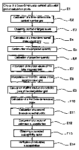
As illustrated by figure 2, this exploitation phase comprises the following
sub-phases:
- obtaining a calculation grid (steps El below);
- constructing a projective quantity (steps E2 to E5 below);
- calibrating the projective quantity (steps E6 below);
- applying the projective quantity to the recorded values (steps E7 to E14
below).
1.1 Obtainingza calculation grid_
In a first step El, a three-dimensional centred calculation grid of
calculation points
of the environment is chosen.
The three steps for the abscissa, ordinate and height of the calculation grid
are
chosen by the user. They are constant, but not necessarily equal to one
another. The size of
the calculation grid is chosen by the user according to the mean measuring
height with
respect to the ground and the detection depth envisaged.
The mean measuring height is 35 m with respect to ground level (as indicated
above). The highest calculation point is for example fixed at 10 m and the
deepest
calculation point at a depth of 43 m (or -43 m in height). A calculation grid
is chosen
extending between the abscissa -160 m and the abscissa 160 m, between the
ordinate -160
m and the ordinate 160 m and between the height -43 m and the height 10 m.
It is chosen to index the abscissa i and the ordinate j every 10 metres, from -
16 to
+16, that is to say 33 indices for the abscissa and for the ordinate (i
between -16 and 16
and j between -16 and 16), and to index the height k every 1 metre for the
height, that is to
say 54 indices (k between 1 and K= 54). Thus each calculation point can be
identified by
its indices (i,j,k).
One level of the calculation grid corresponds to a constant height index and
is
therefore a square table of N*M calculation points (with N = 33 and M = 33).
The
calculation grid comprises 54 levels.
The calculation grid 20 of calculation points 21 used in the location method
according to the first embodiment of the invention is presented in relation to
figure 3. For
CA 02653969 2008-12-01
reasons of simplicity, only the part of the calculation grid corresponding to
the abscissa
indices 22 and ordinate indices 23 ranging from -5 to +5 and to the height
indices 24
ranging from -10 to +5 has been shown.
With each calculation point for indices (i,j,k) of the calculation grid there
is
5 associated a position vector extending from the abscissa and ordinate point
corresponding
to the indices i and j and situated at the magnetometer height (i.e. 35 m) at
the point of
indices (0,0,k). That is to say the vector of coordinates (i,j,(35-11)+k) is
associated with
the calculation point (i,j,k) of the calculation grid. In this way a three-
dimensional position
vector centred grid is obtained.
1.2 Construction of projective quantitX
In a second step E2, a three-dimensional centred number grid is calculated.
Using the approximation of the reduction to the pole defined above, with each
calculation point of indices (i,j,k) of the calculation grid there is
associated a number
obtained from the scalar product of the unitary vector carrying the mean field
Bm and the
total magnetic field vector (or magnetic deviation) at the abscissa and
ordinate point
corresponding to the indices i and j and situated at the height of the
magnetometer (the
first reference point) resulting from a spherical abnormality of pure iron of
one gram
situated at the point of indices (0,0,k) (the second reference point).
The following mathematical formula (3) is used:
B = 1 x(3(M . u) u - M) (3)
r
where B is the local magnetic field, r is the distance, u is the unitary
vector, M the
magnetic moment of a sphere of pure iron (of susceptibility 500000, of mass 1
g and of
radius 3.128 mm), the moment M is carried by the unitary vector.
In the context of the present embodiment, (0,0,11-k) is obtained for the
second
reference point (the position of the sphere) and (10i, lOj, 35) for the first
reference point.
The grid contains 33*33*54 numbers.
In this way a number grid is obtained. In the same way as the calculation
point
grid, each of the numbers is located by its indices (i,j,k) and the number
grid comprises a
CA 02653969 2008-12-01
16
plurality of number levels, a height index of the number grid corresponds to
each number
level.
In a third step E3, for each number level of the number grid corresponding to
a
height index and for each pair of indices (i,j), a enlarged level is obtained
centred at (i,j).
An index number level of height k (between 1 and K=54) of the number grid is
fixed. This number level k is supplemented with zeros in order to obtain an
enlarged level
k longer and wider than the number level k and so that the number level k is
centred at (i,j)
in the enlarged level k.
For example, an enlarged level of 51 points by 51 points is fixed. The number
level
of index k of size 33 by 33 is located in the enlarged number level between
its indices 26-
16 and 26+16 both on the abscissa and on the ordinate.
In a fourth step E4, a three-dimensional angle cosine grid is calculated.
A number level corresponding to a height index kl (k1 between 1 and K) is
fixed.
Next a first vector is obtained from the enlarged level kl centred at (0,0) by
putting
end to end each column of this enlarged level kl centred at (0,0).
For each number level corresponding to a height index k2 (k2 between 1 and K)
and for each index i (between -16 and 16) and j (between -16 and 16), a second
vector is
obtained from the enlarged level k2 centred at (i,j) by putting end to end
each column of
this enlarged level k2 centred at (i,j).
Then there is calculated, for each triplet of index (i,j,k2) where the index
k2 runs
through all the level indices (from 1 to K), the cosine of the angle between
the first vector
and the second vector by the algebraic formula of the scalar product divided
by the
product of the norms. In this way an angle cosine grid is obtained for the
index kl.
This step E4 is repeated for each height index kl (varying from 1 to K = 54).
In a fifth step E5, at least one projective parameter quantity is constructed.
For a height index kl (between 1 and K) and for each of the cosines g(i,j,k2)
of the
angle cosine grid corresponding to this index kl, the pseudo-angle
corresponding to this
cosine is calculated by virtue of the following mathematical formula:
a co )
f(i,j,k2) = 1 s(g(i, j, k 2) (4)
71
CA 02653969 2008-12-01
17
If the cosine of the angle g(i,j,k2) is equal to 1, its image is equal to 1,
and if the
cosine is -l, its image is 0. The image of a cosine by this function is
positive.
Next the vertical curvature of the pseudo angle previously calculated is
defined by
virtue of the following mathematical formula:
-f"
(5)
l+a.f2
where a is a parameter to be tested, f is the vertical first derivative given
by the following
mathematical formula:
f(i, j, k 2) + f(i, j, k 2 - 1) (6)
2
where f' is the second vertical derivative given by the following mathematical
formula:
f(i j, k2 + l) - 2f(i j, k2) + f(i j, k2 - 1) (7)
The first (corresponding to k2 = 1) and last (corresponding to k2 = 54) levels
of the
cosine grid corresponding to the index kl are not calculated since either k2-1
or k2+1 no
longer corresponds to calculated levels of the grid. Norming is carried out by
dividing the
maximum value obtained on the grid. Thus the new maximum value for the grid is
systematically 1.
In this way, for each height index kl (between 1 and K = 54), there is
obtained a
vertical curvature grid that constitutes the projective quantity for the level
kl.
In the present embodiment, the levels corresponding to 10 m of altitude (index
1)
and 43 metres depth (index 54) are not calculated. All the other levels, that
is to say 52
levels, are calculated. The alpha parameter is equal to 1 in the example
chosen.
1.3 Calibration of the projective quantitX
In a sixth step E6, for each index kl (between 1 and K = 54), a calibration of
the
projective quantity is implemented by means of a calculation of the
susceptibility
CA 02653969 2008-12-01
18
equivalents (according to a variant of this first embodiment, the mass
equivalents or
equivalents of parameters proportional to susceptibilities are calculated) in
order to form a
correction grid for the projective quantity.
The pseudo-proportionality formula of two vectors given by the following
mathematical formula is used:
L (u, v) _ u . v (8)
V . V
where u and v are two vectors in the same vectorial space of finite dimension,
and v is
non-zero. When the vector u can be written in the form: k.v where k is a
number, L(u,v) is
equal to the number lambda.
The vector u is the extract of the level kl of the grid situated between
symmetrical
abscissae and ordinates.
The vector v is defined by the following linear combination:
v = a(1).v(l) + a(2).v(2) + ... + a(k).v(k) (9)
The curvatures c(1), c(2) ..., c(k) are the central values of the
aforementioned
vertical curvature grid corresponding to the height index kl. The maximum
value of this
curvature is 1. The family b(l), b(2), ..., b(k) is defined by the following
mathematical
formula:
b(l) - exP(R =co)) (10)
exp(,8)
with (3 a parameter to be fixed.
This is a family of positive numbers, where the sum of all the numbers is
denoted
S.
The family a(l), aO2 b(~ ~
, ..., a(k) defined by a (j)= is a partition, that is to
s
say a finite family of positive numbers of sum 1.
CA 02653969 2008-12-01
19
The vector v(j) corresponds to the level j of the aforementioned number grid
between symmetrical indices, the centre of the number grid being of zero
abscissa and
zero ordinate.
In the present embodiment, the value 2 is chosen for the parameter (3 and the
v(j)
quantities are defined by the square bordered on the abscissa and ordinateby
the indices -
and +10, and u is the level k of the aforementioned number grid, bordered on
the
abscissa and ordinate by -10 and 10.
The number thus obtained is denoted corr(kl). It is a case of the weighting
with
respect to itself of a point abnormality. The index kl runs through 2, 3, ...,
K-l, the first
10 (kl = 1) and last (kl = 54) levels are not calculated.
This number corr(kl) will make it possible to adjust the projective quantity
corresponding to the index kl.
The relationship between the depth, represented by the ordinate axis3l, and
the
equivalent mass, represented by the abscissa axis 32, of the 54 abnormality
levels 33 is
presented in relation to figure 4. It may be noted that the levels 1 and 54
are arbitrarily
zero.
The steps E2 to E6, which concern the construction of a projective quantity
and its
calibration, are substituted for the linear system resolution by matrices well
or poorly
conditioned, adapting to ideal abnormalities the parameters of the various
calculation tools
associated with the various steps.
CA 02653969 2008-12-01
1.4 Application of the projective quantity to the values recorded
In a seventh step E7, the recorded values of the total magnetic field are
imported.
During this step, the recordings of the total field obtained by helicopter are
imported in order to use them in the next steps of the location method
according to the first
5 embodiment of the invention. Each point recorded consists of an abscissa, an
ordinate, the
mean height and the intensity of the total magnetic field recorded at this
point.
In an eighth step E8, an interpolation is carried out of the recorded values
of the
grid of values recorded so as to obtain an interpolation grid comprising
interpolated
values, this interpolation grid comprising the same abscissa, ordinate and
height steps as
10 the calculation grid.
This step E8 of the method makes it possible to obtain a recording of points
with
regular steps corresponding to the steps of the calculation grid.
The abscissa and ordinate step of the calculation grid is used. A calculation
point of
the calculation grid is fixed. The measuring points (each corresponding to a
recorded
15 value) are classified in the increasing order of the distances to this
calculation point.
If several measuring points are exactly at the same distance from the
calculation
point, an order is defined between them. A triplet of distinct measuring
points defined by
their previous rank is taken. Their ranks are added. This sum goes from
6(1+2+3) to N+N-
1+N-2, if N is the number of measurement points.
20 A test is carried out in order to determine whether the triplet of points
is aligned.
When these three points are not aligned the barycentric coordinates of the
interpolation
point of the interpolation grid in the reference frame formed by this triplet
are calculated.
Thus, when these three barycentric coordinates are positive and the sum of the
ranks is minimum among all the triplets fulfilling this barycentric condition,
the positive
weights P 1, P2 and P3 of sum 1 are recorded, and the measurement at the
interpolation
point of the interpolation grid is defined by the barycentre of the three
measurements at the
three measuring points selected, each allocated the weights P1, P2 and P3. In
this way the
triangle of measuring points closest to the current interpolation point of the
interpolation
grid are defined such that the current interpolation point of the
interpolation grid is in this
triangle.
In this first embodiment according to the invention, this algorithm is limited
to the
points adjacent to the recording in order to reduce the interpolation
calculation time.
CA 02653969 2008-12-01
21
In a ninth step E9, a zone G of size N*M is selected in the interpolation grid
and its
affine residue is calculated, by affine projection of this part of the
interpolation grid using
the method of least squares.
In this way the affine residue of this projection is obtained, this affine
residue
comprising a plurality of projected values forming a grid of projected values
of size N*M.
The family of polynomials 1, X and Y defines the vector space of dimension 3
of
the affine functions with two variables. The grids of values representing them
are denoted
G 1, Gx and Gy.
Each of the grids of values G1, Gx, Gy of the functions 1, X and Y are each
converted into a column vector by arranging each of its columns end to end.
The
juxtaposition of the three columns each corresponding to the grids G1, Gx and
Gy forms a
rectangular matrix M1 of 3 columns and N*M rows.
Ml is multiplied by its transpose so as to obtain a matrix M2, with 3 rows and
3
columns. M2 is a Gram matrix. This matrix is inverted and termed M3. The
product of the
matrix M3 and the matrix M1 is calculated, which forms a rectangular matrix
denoted M4.
The selected zone of the interpolation grid of dimensions N*M is transformed
by
the same method as that applied to the grids G1, Gx and Gy into a column
vector V of size
N*M. The product V.M4 is a vector with 1 row and 3 columns.
Let u, v, w be the coordinates of the orthogonal projection of the selected
zone of
the interpolation grid onto the vector space generated by 1, X and Y. There is
substituted
for the selected zone of the interpolation grid the grid of projected values
G2, which is
given by the following mathematical formula:
G2 = G - u.Gl - v.Gx - w.Gy (11)
The projected values grid G2 is the affine projection, by the least squares
method,
of the selected zone of the interpolation grid.
Thus, unlike the conventional techniques for magnetic object location that use
the
affine part of the projection, the method according to the first embodiment of
the invention
uses the residue of the affine projection.
It is considered that the signal is that of the abnormality with the addition
of a
background noise caused by progressive variations in the local geology. It is
these
CA 02653969 2008-12-01
22
progressive variations that tend to be eliminated by subtraction of the affine
function
which is the orthogonal projection onto a grid of fixed length and width of
the magnetic
recording. Reproductions of the field show clearly the disappearance of the
magnetic
background noise.
This makes it possible to obtain a more precise location than the conventional
techniques and makes it possible in particular to distinguish point
abnormalities or
abnormalities of small size and high susceptibility compared with
abnormalities of large
size and low susceptibility, whereas the conventional techniques, in
particular based on
matrix inversion, do not make it possible to make this discrimination.
In a tenth step E 10, a construction of a third vector (otherwise designated
by first
three-dimensional index) is used.
For each number level corresponding to a height index k (between 1 and K= 54)
of
the number grid (level k), the kth coefficient of the third vector is equal to
the scalar
product of the projected value grid G2 and the level k of the number grid.
In an eleventh step El l, the projective quantities are applied to the third
vector in
order to obtain a fourth vector (otherwise designated by second three-
dimensional
magnetic abnormality index).
In a twelfth step E12, a fifth vector is calculated, which is an estimated
susceptibility vector (according to a variant of this embodiment, it is a mass
vector or a
vector of parameters proportional to susceptibilities), by a method similar to
that described
in step E6.
The first and last coefficients of this fifth vector are not calculated, and
their value
is chosen arbitrarily to be equal to 0, since the differential operator (or
projective quantity)
defined in step E5 does not allow calculation of the coefficient for the
highest altitude
(index k = 1) or the deepest depth (index k = 54). The coefficients of this
fifth vector are
denoted susceptibility(1)=0, susceptibility(2), ..., susceptibility(K-1), and
susceptibility(K)=O.
In a thirteenth step E13, a correction to the susceptibility vector is used in
order to
produce a corrected susceptibility vector.
The susceptibility index 40 (on the abscissa axis) and the corrected
susceptibility
index 41 (on the abscissa axis) corresponding the central axis (of coordinates
(11,11)) of
the selected zone (step E9) of the interpolation grid used in the location
method according
CA 02653969 2008-12-01
23
to the first embodiment of your invention are presented in relation to figure
5 as a function
of the depth 43 (on the ordinate axis).
To do this, for each index k between 2 and K-1, the coefficient k of the
corrected
susceptibility vector is obtained by dividing the coefficient k of the
susceptibility vector
denoted susceptibility(k) by the number corr(k) obtained at step E6.
In a fourteenth step E14, a verification of the susceptibilities calculated in
step E13
is implemented.
To do this, a magnetic field is reconstituted by adding to all the tri-indices
(i,j,k)
the variation in the total magnetic field caused by a point abnormality
situated at (i,j,k), the
susceptibility of which is calculated at step E13.
The aforementioned steps E7 to E14 are the application in the real case of the
calculations and adjustments of the aforementioned steps E3 to E6.
The estimated susceptibility vector makes it possible to obtain a location of
said
object.
2. Second embodiment: the case of a reading of the magnetic field gradient
This second embodiment is adapted to the readings made on the ground. It will
be
considered hereinafter that the aforementioned phase of measuring the
measuring points in
the environment is carried out by means of a gradiometer situated at 0.15 m
from the
ground comprising a high magnetometer situated at a height of 0.7 m (first
height) and a
low magnetometer situated at a height of 0.1 m (second height).
The steps of the exploitation phase according to the second embodiment of the
invention are detailed below (the magnetic parameter recorded is the magnetic
field
gradient). As illustrated by figure 6, this exploitation phase comprises the
following sub-
phases:
- obtaining a calculation grid (step Fl below);
- constructing a projective quantity (steps F2 to F7 below);
- calibrating the projective quantity (step F8 below);
- applying the projective quantity to the values read (steps F9 to F13 below).
2.1 Obtaining a calculation grid
CA 02653969 2008-12-01
24
As in the first step El of the first embodiment of the location method
according to
the invention, in a first step Fl of the second embodiment, a three-
dimensional centred
calculation grid of calculation points of the environment is chosen.
The three steps for the abscissa, for the ordinate and for the height of the
calculation grid are chosen by the user. They are constant, but not
necessarily equal to one
another. The size of the calculation grid is chosen by the user according to
the mean
measuring height with respect to the ground and the detection depth envisaged.
The mean measuring height is 0.15 m with respect to ground level (as indicated
above). For example, the highest calculation point is fixed at 0 m and the
deepest
calculation point at a depth of 3.9 m (or a height of
-3.9 m). A calculation grid is chosen extending between the abscissa -5 m and
the abscissa
5 m, between the ordinate -5 m and the ordinate 5 m and between the height -
3.9 m and
the height 0 m.
It is chosen to index the abscissa i every 0.5 m, from -10 to +10, that is to
say 21
indices for the abscissa (i between -10 and 10) and the ordinate j every 0.25
m, from -20 to
+20, that is to say 41 indices for the ordinate (and j between -20 and 20),
and to index the
height k every 0.1 m for the height, that is to say 40 indices (k between 1
and K=40). Thus
each calculation point can be identified by its indices (i,j,k).
The abscissa and ordinate indices are symmetrical, that is to say they go from
an
integer value -n 1 to +n 1, n 1= 10 is the maximum abscissa index, and from -m
l to +m 1
for the ordinate, ml = 20 is the maximum ordinate. The abscissa indices are
therefore
2n1+1 in number, the ordinate indices are 2ml+l in number.
A level of the calculation grid corresponds to a constant height index and is
therefore a square table of NxM (where N = 21 and M = 41) calculation points.
The
calculation grid comprises 401evels.
The calculation grid presented in relation to figure 2 also illustrates the
calculation
grid used in the location method according to the second embodiment of the
invention. For
reasons of simplicity, only the part of the calculation grid corresponding to
the abscissa 22
and ordinate 23 indices ranging from -5 to +5 and to the height indices 24
ranging from -
10 to +5 has been shown.
With each point of calculation of indices (i,j,k) of the calculation grid
there is
associated a position vector extending from the abscissa and ordinate point
corresponding
CA 02653969 2008-12-01
to the indices i and j and situated at the height of the magnetometer (i.e. 35
m) to the index
point (0,0,k). That is to say with the calculation point (i,j,k) of the
calculation grid there is
associated the vector of coordinates (i,j,(35-11)+k). In this way a three-
dimensional
position-vector centred grid is obtained.
5 Naturally, other depths for the deepest calculation point can be chosen in
the
context of the invention.
2.2 Construction of a projectivequantity
In the same way as during step E2 of the first embodiment of the location
method
10 according to the invention, in a second step F2 of the second embodiment, a
three-
dimensional centred number grid is calculated.
By using the approximation of the reduction-to-the-pole described previously,
with
each calculation point of indices (i,j,k) of the calculation grid, there is
associated a number
obtained from the scalar product of the unitary vector carrying the mean field
Bm and the
15 vertical gradient vector of the magnetic field between the abscissa and
ordinate points
(first and second reference points) corresponding to the indices i and j and
situated at the
heights respectively of the high magnetometer and low magnetometer resulting
from a
spherical abnormality of pure iron of 1 gram situated at the index point
(0,0,k) (third
reference point).
20 Once again the mathematical formula (3) previously defined in the context
of the
second step E2 of the first embodiment according to the invention is used.
(0; 0; -0.15 - 10 k) is obtained for the position of the sphere with respect
to the low
magnetometer of the sensor (second height: 0.1 m), and (0.50i; 0.25j; -0.75 -
0.10 k) for
the position of the sphere with respect to the high magnetometer of the sensor
(first height:
25 0.7 m). The number grid contains N*M*K numbers, with N = 21, M = 41 and K =
40.
In this way a number grid is obtained. In the same way as the calculation
point
grid, each of the numbers is referenced by its indices (i,j,k) and the number
grid comprises
a plurality of number levels, to each number level there corresponds a height
index of the
number grid.
In a third step F3, there is constructed a filtering grid (also called a
weighting grid)
of filtering numbers in the form of a three-dimensional matrix containing
N*M*K filtering
numbers (with N = 21, M = 41 and K = 40).
CA 02653969 2008-12-01
26
For each level of the filtering grid corresponding to a height index k, a
parameter 8
is defined corresponding to a distance and dependent on the depth, for example
8(k) = 0.75
+ 0.07 k (the coefficients 0.75 and 0.07 of this affine expression of the
parameter 6 are
obtained after numerous tests and simulations).
For a level of the filtering grid corresponding to the height index k, the
value S(k)
is calculated. In the level k, the distance between the origin (0, 0) and the
abscissa and
ordinate point (i, j) is given by the expression: i2+ j2 . The filtering
number
corresponding to the indices (i,j,k) of the filtering grid is then defined by:
~ + j2 1
max (O 1- ~~ kz1 (12)
J
O )
Expression (12) always takes the value 1 in (0,0,k) whatever the value of k.
This filtering grid forms a safety cone broadening towards the base.
The levels 51, 52, 53 corresponding respectively to the values of the
parameter S
0.9, 0.5 and 0.05 of the cone are represented by transparency on a square base
with sides
of 5 m and a depth of 0 to 4 m on the diagram in figure 7.
In a fourth step F4, a Gram matrix is constructed from a filtering by means of
a
filtering grid of the number grid.
A first filtered grid C(i,j,k) is calculated by virtue of the tensor product
defined by
the following equation:
C(i,j,k) =A(i,j,k) = B(i,j,k) (13)
where A(i,j,k) and B(i,j,k) correspond to the number and filtering grids
containing
N*M*K numbers defined respectively during steps F2 and F3 (with N = 21, M = 41
and K
= 40).
In this way the first three-dimensional filtered grid of filtered numbers
C(i,j,k) is
obtained.
CA 02653969 2008-12-01
27
Each of the K levels of the first filtered grid is then transformed into an
N*M row
vector by putting each column of this level end to end. In this way a
rectangular matrix
M1 with N*M rows and K columns is obtained.
Each column vector of the matrix M1 is divided by its Euclidian norm in order
to
result in a new matrix M2.
Then the matrix M2 is multiplied by its transpose so as to obtain a square
matrix
M3 with K rows and K columns, M3 being a first matrix that is a Gram matrix.
The
diagonal coefficients of the first matrix M3 are all equal to I since they
correspond to the
square of the Euclidian norm of the column vectors of the matrix M2, these
vectors being
normed during the passage from M1 to M2.
In a fifth step F5, a combined matrix M4 corresponding to a combination of the
first matrix M3 with an identity matrix Id with the same dimensions as the
first matrix M3.
This combined matrix M4( ) is defined by the following equation:
M4(p) = 1 Id+ M 3 (14)
+ 1 + 1
where is a positive or zero number to be tested and Id the identity matrix
with K rows
and K columns.
M4( ) thus corresponds to a barycentric combination with positive weights of
Id
and M3. All the diagonal terms of the combined matrix M4 are equal to 1. This
is because
this matrix is the barycentre of the two matrices M3 and Id, which are both
with diagonal
coefficients equal to 1.
Unlike the matrix M3, the matrix M4 is now well conditioned.
The number is chosen for example equal to 6.
In a sixth step F6, a pseudo-inversion matrix M6 is constructed.
First of all the combined matrix M4( ) defined above is inverted. An inverted
matrix M5 is then obtained.
By multiplication of the inverted matrix M5 by the matrix M2, the pseudo-
inversion matrix M6 is obtained, which is a rectangular matrix with N*M rows
and K
columns.
CA 02653969 2008-12-01
28
In a seventh step F7, at least one projective quantity with parameter is
constructed.
An intermediate number grid is constructed, the abscissa indices of which
extend
from -n2 to n2 and the ordinate indices from -m2 to m2 with n2 strictly
greater than nl
and m2 strictly greater than ml, the integers n 1 and ml being previously
defined in step
Fl. The height index of this intermediate grid extends from 0 to K. For
example nl = 15
and m2 = 30 are chosen.
To do this, an index iO between -n2+nl and n2-nl is selected, and an index jO
between -m2+m1 and m2-ml, and an index kO between 1 and K, the index level kO
of the
number grid (of step F2) is positioned between the indices i0-nl and iO+nl, j0-
ml and
jO+ml in the intermediate grid so as to obtain the number level of index kO in
the
intermediate grid.
The number level of index kO of the intermediate grid thus obtained is
duplicated
on the K levels of this intermediate grid in order to obtain a three-
dimensional
intermediate number grid. The tensor product of this intermediate grid
obtained by the
filtering grid of step F3 is then calculated in order to obtain a filtered
intermediate grid.
For each height index k (k between 1 and K), the level k of the filtered
intermediate
grid corresponding to a vector with N*M rows is transformed by putting the
columns of
this level end to end. In this way a matrix Ml' with K columns and N*M rows is
obtained.
By dividing each column vector of M1' by its own norm, the matrix M2' results.
This matrix M2' is next multiplied by the matrix M6, defined during the above
step
F6, in order to supply a square matrix M7 of dimension K.
Then M6 is multiplied by the matrix M2' in order to obtain a square matrix M8
with K rows and K columns.
The matrix M7 is then multiplied by the transpose of the matrix M8. Then a
square
matrix M9 is obtained.
Then the matrices M7 and M8 are multiplied by their own transpose in order to
give two square symmetrical matrices, denoted respectively M10 and M11.
Then the geometric index in (iO, jO, kO) is used to designate the number
defined by
the following expression:
G1 (i0, j0, k0) M9(k0, k0) _ (15)
M10(k0, k 0) o M11(k0, k0)
CA 02653969 2008-12-01
29
Thus the matrix M7 constitutes a first vector and the transpose of the matrix
M8 a
second vector.
This equation 15, which corresponds to a scalar product of the first vector
and the
second vector divided by the product of the norms of the first and second
vectors is an
angle cosine whose value is between -1 and +1.
For each of the triplets (i,j,k), the pseudo-angle f(i,j,k) corresponding to
the cosine
of the expression (24) is calculated in (ij,k) by means of the following
mathematical
formula:
a cos(G 1(i, j, k) )
f(i,j,k) = 1 - (16)
7r
If the cosine of the angle G1(i,j,k) is equal to 1, its image is equal to 1,
and if the
cosine is equal to -1 its image is equal to 0. A three-dimensional grid of
pseudo-angles
f(i,j,k) denoted G2 is obtained.
Next the vertical curvature G3(i,j,k) of the pseudo-angle previously
calculated is
defined by means of the following mathematical formula:
G3 (i,j,k) = - f (17)
1 + 2 f
where a,2 is a parameter to be tested (it is chosen for example equal to 1), f
is the first
vertical derivative given by the following mathematical formula:
f(i, j, k) + f(i, j, k
1) (18)
2
and f' is the second vertical derivative given by the following mathematical
formula:
f(i j,k+1)-2f(i j,k)+f(i j,k-1) (19)
CA 02653969 2008-12-01
The first (corresponding to k = 1) and last (corresponding to k= K) variables
of the
grid G2 defined above are not calculated, the value 0 is arbitrarily
attributed to them. In
this way a grid G3 of vertical curvatures is obtained.
Normalizing is carried out by dividing the maximum value obtained on the grid
5 G3. Thus the maximum value obtained on the grid is systematically 1. This
new grid that
constitutes the projective quantity is denoted G4.
2.3 Calibration of the projective quantity
In an eighth step F8, a calibration of the projective quantity is implemented
by
10 means of a calculation of the susceptibility equivalents (according to a
variant of this
second embodiment, the mass equivalents or equivalents of parameters
proportional to
susceptibilities are calculated) in order to form a correction grid of the
projective quantity.
The vector V 1 is considered, a vertical vector corresponding to the central
column
of the grid G4 (that is to say of the projective quantity). The vector Vl has
40 height
15 indices since there are 401evels in the grid G4 (K = 40) where each of
these coordinates is
no more than 1.
The vector V2 with K positive height indices (with K= 40) is defined by the
following equation:
20 V2(k)=exp(~3. Vl (k)) k=1,2,...,K (20)
The vector V3 is defined by the following mathematical expression:
V3(k) = V 2(k) k--1,2,...,K (21)
V 2 (1) + V 2 (2) + . . . + V 2(K)
where each of the K coordinates of this vector V3 is positive and the sum of
all the
coordinates of V3 equal to 1.
The vertical reference gradient is defined by the following barycentric
combination:
C4(k)=V3(1)xC(1)+V3(2)xC(2)+...+V3(K)xC(K)
CA 02653969 2008-12-01
31
(22)
where C(k) is the extract of the level k of the number grid calculated during
step F2, that is
to say the vertical gradient grid of a spherical abnormality of 1 gram of pure
iron situated
at the index of height k multiplied by the vertical step defined at F1.
The vertical field gradient C(k) of level k and the reference vertical
gradient C4(k)
for this level, which are grids of abscissa between -nl and +nl and ordinate
between -ml
and +ml, are transformed into a vector of size N*M.
As during step E6 of the first embodiment, use is made in the aforementioned
pseudo-proportionality formula (in relation to step E6) in order to calculate
the pseudo-
proportionality index of the vertical gradient C(k) of level k with respect to
the reference
vertical gradient C4(k) of level k by virtue of the following expression:
Correction(k) = < C (k) , C 4 (k) > (23)
< C4(k), C 4 (k) >
where (.,.) designates the canonical scalar product with C(k) and C4(k) two
vectors of the
same vectorial space of finite dimension, C4(k) is non-zero. When the vector
C(k) can be
written in the form: k.C4(k) where k is a number, Correction(k) is equal to
the number
lambda.
This step is repeated for each height index k (varying from 1 to K). In the
example
chosen, nl is equal to 10 and ml is equal to 20, the coefficient lambda3 is
equal to 2.
This number Correction(k) will make it possible to adjust the projective
quantity
corresponding to the index k.
There is presented, in relation to figure 8, the logarithm of the pseudo-
proportionality index Correction(k) 62 as a function of the depth 61 (abscissa
axis).
2.4 Application of the projective quantity to the values of the recording's
In a ninth step F9, a grid of recorded values of the vertical magnetic field
gradient
is calculated from the magnetic map of recorded values of the vertical
magnetic field
gradient. The coordinates (i, j) in the magnetic map correspond to the point i
multiplied by
the abscissa step and j multiplied by the ordinate step.
CA 02653969 2008-12-01
32
Unlike the location method according to the first embodiment (the case of the
total
field and the helicopter reading), in the location method according to this
second
embodiment, a step of interpolation of the recorded values so as to obtain an
interpolation
grid is not implemented.
In a tenth step F10, for a pair (i,j) chosen in the recorded value grid, a
zone is
selected delimited by the indices i-nl and i+nl, and j-ml and j+ml, and its
affine residue
is calculated by affine projection of this delimited zone of the recorded
value grid by
implementing the method of least squares as described in relation to step E9
of the first
embodiment.
The affine residue of this projection is obtained, this affine residue
comprising a
plurality of projected values forming a projected value grid of size N*M.
This projected value grid is duplicated on K levels. A transformed three-
dimensional grid of N rows, M columns and K levels is then obtained, each of
the K levels
being identical to all the others.
The tensor product of this three-dimensional grid transformed by the filtering
grid
calculated at step F3 is then effected. A second filtered three-dimensional
grid is then
obtained.
By using the technique applied to the first filtered matrix in the fourth step
F4, in
an eleventh step F 11, the second filtered three-dimensional grid (obtained in
step F 10) is
modified as a matrix of N*M rows and K columns called Ml', by transforming
each of the
K levels of this second filtered grid into a column vector.
Each column vector of this matrix Ml' is then divided by its norm and thus a
matrix M2' is obtained.
Next this matrix M2' is multiplied by the matrix M6 calculated at step F7.
Then a
square matrix with K rows and K columns denoted M7' is obtained.
The matrix M6 is next multiplied by the matrix M2' in order to obtain a square
matrix M8 of K rows and K columns.
The product of the matrix M7' and the transpose of the matrix M8' supplies the
square matrix M9' of size K, and the product of the matrices M7' and M8'
multiplied by
their transpose supplies respectively the symmetrical square matrices M10' and
M11'.
The geometric index in (i0,j0,k0) designates the number defined by the
following
expression:
CA 02653969 2008-12-01
33
G1' (i0, j0, k0) = M 9' (k, k) (24)
M 10 '(k, k) = M 11 '(k, k)
Thus the matrix M7' constitutes a first vector and the transpose of the matrix
M8' a
second vector.
This equation (24), which corresponds to a scalar product of the first vector
and the
second vector divided by the product of the norms of the first and second
vectors, is an
angle cosine and its value is between -1 and +1.
For each of the triples (i,j,k), the pseudo angle fl(i,j,k) corresponding to
the cosine
of expression (24) in (i,j,k) is calculated by means of the following
mathematical formula:
a cos(G 1' (i, j, k) )
fl (ij,k) = 1 - (25)
7u
If the cosine of the angle Gl(i,j,k) is equal to 1, its image is equal to 1,
and if the
cosine is equal to
-1, its image is equal to 0. The grid of the pseudo-angles fl (i,j,k) is
denoted G2.
Using the expression (17) (defined in relation to step F7), the vertical
curvature
G3'(i,j,k) of the pseudo-angle previously calculated is next obtained.
The first (corresponding to k= 1) and last (corresponding to k= K) levels of
the
grid G2' defined above are not calculated, and the value 0 is attributed to
them arbitrarily.
Then the three-dimensional grid G3' of vertical curvatures is obtained.
Next a three-dimensional grid G4' is defined, with the same size as G3',
attributing
to each tri-index (i,j,k) the value 1 when the second derivative on the
abscissa is defined
by the following mathematical formula:
G3'(i+l j,k)-2G3'(i,j,k)+G3'(i-l,j,k) (26)
and the second derivative on the ordinate defined by the following
mathematical formula:
G3'(i,j+l,k)-2G3'(i,j,k)+G3'(i,j-l,k) (27)
CA 02653969 2008-12-01
34
are negative or zero, and 0 in the contrary case.
Next the tensor product of G4' and G3' is effected in order to obtain a three-
dimensional grid G5'.
In a twelfth step F12, a vector of estimated susceptibilities is calculated
(according
to a variant of this embodiment, it is a mass vector or a vector of parameters
proportional
to susceptibilities).
To do this, a sub-grid of appropriate size is selected from the grid of
recorded
values of the vertical gradient of the two-dimensional magnetic field. This
zone is situated
between the abscissae i-nl and i+nl and between the ordinates j-ml and j+ml.
Then the
affine residue of this sub-grid is calculated in the same way as in step F10.
In the same way as in step F7, the angle cosine vector (also referred to as
the
geometric index vector) is determined, comprising K height indices, from the
grid G5'
defined in step F11 above.
As in step F8, from the reference vertical gradient, the pseudo-
proportionality
index of the affine residue of the zone is determined with respect to the
reference vertical
gradient.
Next the pseudo-proportionality index is multiplied by the angle cosine vector
in
order to result in the vector Susceptibilityl.
Finally, each k-th coordinate of the vector Susceptibilityl is divided by the
corresponding corrective term Correction(k) determined at step F8. Then the
vector
susceptibility2 is obtained.
In a thirteenth step F13, a verification of the susceptibilities calculated in
step F12
is implemented.
To do this, a magnetic field is reconstituted by adding to all the tri-indices
(i,j,k)
the variation in the total magnetic field caused by a point abnormality
situated at (i,j,k) and
the susceptibilities of which are calculated at step F12.