Note: Descriptions are shown in the official language in which they were submitted.
CA 02712873 2014-03-26
METHOD OF ARTIFICIAL NEURAL NETWORK LOADFLOW COMPUTATION FOR
ELECTRICAL POWER SYSTEM
TECHNICAL FIELD
[001] The present invention relates to method of Artificial Neural Network
Loadflow (ANNL)
computation in power flow control and voltage control in an electrical power
system.
BACKGROUND OF THE INVENTION
[002] The present invention relates to power-flow/voltage control in
utility/industrial power
networks of the types including many power plants/generators interconnected
through
transmission/distribution lines to other loads and motors. Each of these
components of the power
network is protected against unhealthy or alternatively faulty, over/under
voltage, and/or over
loaded damaging operating conditions. Such a protection is automatic and
operates without the
consent of power network operator, and takes an unhealthy component out of
service by
disconnecting it from the network. The time domain of operation of the
protection is of the order
of milliseconds.
[003] The purpose of a utility/industrial power network is to meet the
electricity demands of its
various consumers 24-hours a day, 7-days a week while maintaining the quality
of electricity
supply. The quality of electricity supply means the consumer demands be met at
specified voltage
and frequency levels without over loaded, under/over voltage operation of any
of the power
network components. The operation of a power network is different at different
times due to
changing consumer demands and development of any faulty/contingency situation.
In other words
healthy operating power network is constantly subjected to small and large
disturbances. These
disturbances could be consumer/operator initiated, or initiated by overload
and under/over voltage
alleviating functions collectively referred to as security control functions
and various optimization
functions such as economic operation and minimization of losses, or caused by
a fault/contingency
incident.
[004] For example, a power network is operating healthy and meeting quality
electricity needs of
its consumers. A fault occurs on a line or a transformer or a generator which
faulty component gets
isolated from the rest of the healthy network by virtue of the automatic
operation of its protection.
1
3/26/2014
CA 02712873 2014-03-26
Such a disturbance would cause a change in the pattern of power flows in the
network, which can
cause over loading of one or more of the other components and/or over/under
voltage at one or
more nodes in the rest of the network. This in turn can isolate one or more
other components out of
service by virtue of the operation of associated protection, which disturbance
can trigger chain
reaction disintegrating the power network.
[005] Therefore, the most basic and integral part of all other functions
including optimizations in
power network operation and control is security control. Security control
means controlling power
flows so that no component of the network is over loaded and controlling
voltages such that there
is no over voltage or under voltage at any of the nodes in the network
following a disturbance
small or large. As is well known, controlling electric power flows include
both controlling real
power flows which is given in MWs, and controlling reactive power flows which
is given in
MVARs. Security control functions or alternatively overloads alleviation and
over/under voltage
alleviation functions can be realized through one or combination of more
controls in the network.
These involve control of power flow over tie line connecting other utility
network, turbine
steam/water/gas input control to control real power generated by each
generator, load shedding
function curtails load demands of consumers, excitation controls reactive
power generated by
individual generator which essentially controls generator terminal voltage,
transformer taps control
connected node voltage, switching in/out in capacitor/reactor banks controls
reactive power at the
connected node.
[006] Control of an electrical power system involving power-flow control and
voltage control
commonly is performed according to a process shown in Fig. 7, which is a
method of
forming/defining and solving a loadflow computation model of a power network
to affect control
of voltages and power flows in a power system comprising the steps of:
Step-10: obtaining on-line/simulated data of open/close status of all switches
and circuit breakers
in the power network, and reading data of operating limits of components of
the power
network including maximum Voltage X Ampere (VA or MVA) limits of transmission
lines and transformers; and PV-node, a generator-node where Real-Power-P and
Voltage-
Magnitude-V are given/assigned/specified/set, maximum and minimum reactive
power
generation capability limits of generators, and transformers tap position
limits, or stated
2
3/26/2014
CA 02712873 2014-03-26
alternatively in a single statement as reading operating limits of components
of the power
network,
Step-20: obtaining on-line readings of given/assigned/specified/set Real-Power-
P and Reactive-
Power-Q at PQ-nodes, Real-Power-P and voltage-magnitude-V at PV-nodes, voltage
magnitude and angle at a reference/slack node, and transformer turns ratios,
wherein said
on-line readings are the controlled variables/parameters,
Step-30: performing loadflow computation to calculate, depending on loadflow
computation model
used, complex voltages or their real and imaginary components or voltage
magnitudes or
their corrections and voltage angles or their corrections at nodes of the
power network
providing for calculation of power flow through different components of the
power
network, and to calculate reactive power generation and transformer tap-
position
indications,
Step-40: evaluating the results of Loadflow computation of step-30 for any
over loaded power
network components like transmission lines and transformers, and over/under
voltages at
different nodes in the power system,
Step-50: if the system state is acceptable implying no over loaded
transmission lines and
transformers and no over/under voltages, the process branches to step-70, and
if
otherwise, then to step-60,
Step-60: correcting one or more controlled variables/parameters set in step-20
or at later set by the
previous process cycle step-60 and returns to step-30,
Step-70: affecting a change in power flow through components of the power
network and voltage
magnitudes and angles at the nodes of the power network by actually
implementing the
finally obtained values of controlled variables/parameters after evaluating
step finds a
good power system or stated alternatively as the power network without any
overloaded
components and under/over voltages, which finally obtained controlled
variables/parameters however are stored for acting upon fast in case a
simulated event
actually occurs or stated alternatively as actually implementing the corrected
controlled
variables/parameters to obtain secure/correct/acceptable operation of power
system.
[007] Overload and under/over voltage alleviation functions produce changes in
controlled
variables/parameters in step-60 of Fig. 7. In other words controlled
variables/parameters are
3
3/26/2014
CA 02712873 2014-03-26
assigned or changed to the new values in step-60. This correction in
controlled
variables/parameters could be even optimized in case of simulation of all
possible imaginable
disturbances including outage of a line and loss of generation for corrective
action stored and made
readily available for acting upon in case the simulated disturbance actually
occurs in the power
network. In fact simulation of all possible imaginable disturbances is the
modern practice because
corrective actions need be taken before the operation of individual protection
of the power network
components.
[008] It is obvious that loadflow computation consequently is performed many
times in real-time
operation and control environment and, therefore, efficient and high-speed
loadflow computation
is necessary to provide corrective control in the changing power system
conditions including an
outage or failure of any of the power network components. Moreover, the
loadflow computation
must be highly reliable to yield converged solution under a wide range of
system operating
conditions and network parameters. Failure to yield converged loadflow
solution creates blind spot
as to what exactly could be happening in the network leading to potentially
damaging operational
and control decisions/actions in capital-intensive power utilities.
[009] The power system control process shown in Fig. 7 is very general and
elaborate. It includes
control of power-flows through network components and voltage control at
network nodes.
However, the control of voltage magnitude at connected nodes within reactive
power generation
capabilities of electrical machines including generators, synchronous motors,
and
capacitor/inductor banks, and within operating ranges of transformer taps is
normally integral part
of loadflow computation as described in "LTC Transformers and MVAR violations
in the Fast
Decoupled Load Flow, IEEE Trans., PAS-101, No.9, PP. 3328-3332, September
1982." If
under/over voltage still exists in the results of loadflow computation, other
control actions, manual
or automatic, may be taken in step-60 in the above and in Fig. 7. For example,
under voltage can
be alleviated by shedding some of the load connected.
[010] The prior art and present invention are described using the following
symbols and terms:
Ypq = Gpq jBpq : (p-q) th element of nodal admittance matrix without shunts
Ypp = Gpp jBpp : p-th diagonal element of nodal admittance matrix without
shunts
4
3/26/2014
CA 02712873 2014-03-26
yp = gp jbp : total shunt admittance at any node-p
Vp = ep + jfp = VpZ0p : complex voltage of any node-p
PP + iQp : net nodal injected power
RP p + jRQp : modified net nodal power injection specified
: rotation or transformation angle
[RP] : vector of modified real power injections at power-network
nodes
[RQ] : vector of modified reactive power injections at power-
network nodes
: number of PQ-nodes
: number of PV-nodes
n=m+k+ 1 : total number of nodes
ep : q is the node adjacent to node-p excluding the case of q=p
[ [ : indicates enclosed variable symbol to be a vector or a
matrix
PQ-node: load-node, where, Real-Power-P and Reactive-Power-Q are specified
PV-node: generator-node, where, Real-Power-P and Voltage-Magnitude-V are
specified
Loadflow Computation: Each node in a power network is associated with four
electrical quantities,
which are voltage magnitude, voltage angle, real power, and reactive power.
The loadflow computation involves calculation/determination of two unknown
electrical quantities for other two given/specified/scheduled/set/known
electrical quantities for each node. In other words the loadflow computation
involves determination of unknown quantities in dependence on the
given/specified/scheduled/ set/known electrical quantities.
Loadflow Model : a set of equations describing the physical power network and
its operation for
the purpose of loadflow computation. The term loadflow model' can be
alternatively referred to as 'model of the power network for loadflow
computation'. The process of writing Mathematical equations that describe
physical power network and its operation is called Mathematical Modeling. If
the equations do not describe/represent the power network and its operation
accurately the model is inaccurate, and the iterative loadflow computation
method could be slow and unreliable in yielding converged loadflow
computation. There could be variety of Loadflow Models depending on
organization of set of equations describing the physical power network and its
3/26/2014
CA 02712873 2014-03-26
operation, including Newton Raphson Loadflow (NRL) Model, and Supert
Super Decoupled Loadflow (SSDL) Model.
Loadflow Method: sequence of steps used to solve a set of equations describing
the physical power
network and its operation for the purpose of loadflow computation is called
Loadflow Method, which term can alternatively be referred to as loadflow
computation method' or 'method of loadflow computation'. One word for a set
of equations describing the physical power network and its operation is:
Model. In other words, sequence of steps used to solve a Loadflow Model is a
Loadflow Method. The loadflow method involves definition/formation of a
loadflow model and its solution. There could be variety of Loadflow Methods
depending on a loadflow model and iterative scheme used to solve the model
including Newton Raphson Loadflow (NRL) Methods, Supert Super
Decoupled Loadflow (SSDL) Method.
Artificial Neural Network
[011] Neural Network (NN) based prior art loadflow methods of the kind carried
out as step-30 in
Fig 7 are described in "Stochastic Load Flow Analysis Using Artificial Neural
Networks, 2006
IEEE" by A.Jain, S.C.Tripathy, R.Balasubramanian, and Y.Kawazoe; "Radial basis
function
neural network for power system load-flow, Electrical Power and Energy Systems
30 (2008) 60-
66" by A.Karami and M.S. Mohammadi, and "Artificial neural networks for load
flow and
external equivalents studies, Electric Power Systems Research (2010) article
in press" by
H.H.Muller, M.J.Rider and C.A.Castro. In the above publications and others,
various type of
Artificial Neural Networks (ANNs) involved in loadflow computation are
Multilayer Perceptron
(MLP), Radial Basis Function (RBF), Counter Propagation (CP) and Hopefield
model. Detailed
description of various ANNs and their training, and testing and validation
process is available in
"Principles of Neurocomputing for Science and Engineering, McGrow-Hill (2001)"
by Fredric M.
Ham and Ivica Kostanic, and Principles of Artificial Neural Networks, World
Scientific
Publication (2007)" by Daniel Graupe. Testing and validation of a trained ANN
is to check if the
trained ANN has learned to give accurate enough output data set/vector for a
given input data
set/vector, which was not used in the training process. It is intended to keep
basic description of
Artificial Neural Network and its training process short except inventive
parts.
6
3/26/2014
CA 02712873 2014-03-26
[012] ANN is considered as an important technique of artificial intelligence.
In recent years,
ANNs have gained wide spread attention and they are being used successfully in
many areas of
power systems. Since the first research paper "Artificial neural-net based
dynamic security
assessment for electric power systems, IEEE Trans. Power System 4 (1) (1989)
220-226" by
D.J.Sobajic and Y.H.Pao published, increasing literature demonstrates the
potential of ANN
especially in applications that take advantage of the speed of ANNs for on-
line calculations and
their inherent capacity to overcome modeling complexity. ANN can model any
nonlinear function
of a device or a system described/expressed by a nonlinear equation or
simultaneous nonlinear
equations without knowledge of the actual model structure. ANNs can learn
complex non-linear
relationships among variables/parameters of nonlinear equations through a set
of input/output
examples, and can approximate nonlinear functional relationship among power
system or in
general any device or system variables/parameters of interest. An invention of
artificial (not actual
operational data statistics stored over long period of time like long term,
short term, and daily load
curves) generation of input and output data sets/vectors by different
multiplication factors applied
to operational variables/parameters of a power system described by
simultaneous nonlinear
loadflow equations comprising simulation of feasible and continuous nonlinear
operating region
of the power system for the purpose of training, testing and validating,
forming/defining, and
storing ANN computation model, and then solving said stored ANN computation
model using
general purpose computing apparatus can also be extended in general to any
device or system. It
can be said that outputs of a conventional loadflow method like NRL or SSDL
are functions of the
operating conditions of a power system, and ANNs can be employed to
approximate these
functions. An attractive feature of the ANN loadflow computation is that there
is no possibility of
non-convergence as it might occur with iterative methods like NRL and SSDL
described in "Super
Super Decoupled Loadflow, Presented at IEEE International Conference ¨ Science
and
Technology for Humanity (TIC-STH 2009), pp.252-259" by Suresh B. Patel. Once
an ANN is
trained, it gives output in negligible time by simple direct arithmetic
operations on a given set of
inputs of power system operating condition. The ANN Loadflow can replace the
conventional
NRL and SSDL methods in real time power system operation where time
constraints are very
restrictive.
7
3/26/2014
CA 02712873 2014-03-26
[013] Artificial Neural Networks (ANNs) can be considered as information
processing systems
composed of varying number of simple elements called Neurons distributed into
layers. Neurons
are organized in an input layer, one or more hidden layers, and an output
layer. The connections
between elements largely determine network function just as in natural
biological nervous systems
from which ANNs are inspired. ANN is an intelligent technique that mimics the
functioning of a
human brain, and emulates human intuition of making decisions and drawing
conclusions even
when presented with complex, noisy, irrelevant and partial information. The
structure of an ANN
with only one hidden layer is depicted in Fig.1, which is generic and abstract
with learning,
memorizing and adapting characteristic. The neurons in Fig. 1 are connected to
each other by
weighted links over which signals can pass. Each neuron receives multiple
inputs from other
neurons, except the neurons in the input layer, in proportion to their
connection weights and then
generates a single output in accordance with an activation function. An
activation function can be
linear or nonlinear depending on application. Sigmoid or Hyperbolic Tangent
activation function is
generally used for better performance of ANNs in power system applications.
The weights of
weighted links from a neuron from input to hidden layer is defined as Win, and
the weights of
weighted links from a neuron from hidden to output layer is defined as Who.
The total number of
neurons in input, hidden and output layers are Ik, hk, and Ok, respectively,
where subscript k takes
values of 1 to p, q, and r respectively meaning each layer has different
number of neurons as
shown in Fig. 1. The number of neurons in input layer is the same as number of
input
variables/parameters, the number of neurons in output layer is the same as
number of outputs
variables/parameters, and the number of neurons in hidden layer is determined
experimentally.
[014] An ANN can be trained to perform a particular function by adjusting
values of the
interconnections called weights, and neuron thresholds. The process of
adjusting interconnection
weights and neuron thresholds to achieve output of the ANN the same as the
target value or
desired output for a given input as depicted in Fig. 2 is called training of
ANN. Training of an
ANN consists of adjusting interconnection weights of neurons using a learning
algorithm. Back
propagation with momentum is the commonly used learning algorithm. Multilayer
Feed Forward
ANNs with Error Back Propagation learning algorithm are commonly used in power
system
applications. Feed Forward calculations, and propagating error from output
layer to input layer and
weight updating in hidden and output layers are major steps of training
algorithm. ANNs are also
8
3/26/2014
CA 02712873 2014-03-26
sometimes referred to as Neural Networks (NNs). Anybody skilled in the art of
the process of
training, testing and validating, forming/defining, storing, and then solving
prior art or invention
based ANN model of a device or a system or the power system knows that the
process is carried
out using general purpose single/multi processor computing apparatus. A
General purpose
computing apparatus is a computer that can be used for developing/creating,
testing, and running
different types of programs like word, excel, power point, different browser
programs like Internet
Explorer and Chrome for surfing on Internet (World Wide Web), and even
different types of
Loadflow Computation Programs, and many other types of programs.
[015] The prior art ANN training process can be divided into four modules. The
training, and
testing and validating process is carried out off-line, and it is the
supervised process.
1. Definition of Input and Output data sets/vectors: The prior art ANN
Loadflow method
of "Artificial neural networks for load flow and external equivalents studies,
Electric Power
Systems Research (2010) article in press" by H.H.Muller, M.J.Rider and
C.A.Castro,
suggest the input data vector of dimension 2(m+k+1) given below.
Gd = vg2GdNORM _ pLNORM pgpvNORM cvp (1)
Bd = _va2BdNORM _ QLNORM cvg (2)
Where, GaN Rm and BaN Rm are the diagonal elements of conductance and
susceptance
matrices, normalized with respect to the respective largest element in base
case. Load
powers PLN Rm and QLNoRm as well as generation power Pg are also normalized
with
respect to their base case values. Voltages of generator buses Vg are also
included.
Contingency information is also added to equations (1) and (2) through CVp and
CVq. The
authors write, "This additional information was included to compensate the
loss of
information associated to changes in off-diagonal terms of the admittance
matrix." The
definition of equations (1) and (2) is given in the same language of authors.
2. Training, and Testing and Validating data modeling: The idea of simulating
daily load
curve is used for generating training, and testing and validating data
sets/vectors.
Therefore, for each training and testing and validating demand profile, there
is a base case
and a set of contingencies, in order to simulate possible cases that could
occur in practice.
9
3/26/2014
CA 02712873 2014-03-26
For the training data, the load range is defined as [0.75 ¨ 1.25] pu. As for
testing and
validating data, this range is defined as [0.73 ¨ 1.27] pu, taking into
account that the testing
and validating data should be different from those of training. These load
ranges are
applied simultaneously for all buses. For each input data set/vector
representing power
system operating condition, conventional loadflow computation by method like
NRL or
SSDL method is performed in off line mode to obtain corresponding output data
set/vector.
Contingencies that result in islanding, multiple contingencies, voltage
magnitudes below
0.75 pu, and angles outside greater and beyond ¨80 and +80 are not
considered for
either the training, and testing and validating data sets/vectors.
3. Run and error control: Each pair of input data set/vector of power system
operating
condition and corresponding output data set/vector of loadflow computation
used as target
or desired output is applied to ANN normally simulated on computer. The
process of this
step requires initialization of minimum number of neurons in hidden layer, and
random
synaptic weights of interconnections of neurons. Number of neurons in input
layer is
decided by number of elements of input data set/vector, and number of neurons
in output
layer is decided by number of elements of output data set/vector. With the
initialization
number of neurons in hidden layer, random synaptic weights of interconnections
and
application of input data set/vector, feed-forward action of the ANN generates
or
calculates its output data set/vector, which is compared against the target
data set/vector as
in Fig.2. Error of this comparison is feed back by Back Propagation with
momentum using
steepest gradient descent technique or second order Levenberg-Marquardt
algorithm to
update the interconnection weights and threshold of neurons. This process is
continued
iteratively until error produced is acceptably small for all input/output data
sets/vectors
generated for training of ANN. Trained ANN is then tested and validated if it
has learned to
produce accurate enough output data sets/vectors for a given set of input data
sets/vectors
which are different than those used in training. In testing and validating
phase, error in
output data set/vector is not feedback to update weights of interconnection of
neurons. If
the error vector in testing and validating phase is not small enough further
training is
carried out followed again by testing and validating phase. This process of
training
followed by testing and validating is iterated until testing and validating
phase produce
errors acceptably small enough, and the best ANN is stored in terms of values
of
3/26/2014
CA 02712873 2014-03-26
interconnection weights and_number of neurons in different layers for actual
use in solving
problems for which it is trained. However, for a given set of inputs data
sets/vectors the rate
of convergence of training, and testing and validating process largely depends
upon the
number of hidden neurons, learning rate, momentum factor, and the initial
values of
synaptic weights. Clearly, the proper choice of all these parameters is very
difficult and
involves too many trials as well as uncertainties leading to several thousands
of iterations
for the convergence of training, and testing and validating process.
4. Processing Results: Stored ANN in terms of values of interconnection
weights, number of
neurons in different layers and its performance is analyzed and recorded
errors are shown
and plotted for future reference and possible use.
Calculation steps of Prior Art ANNL method:
[016] The steps of ANN Loadflow computation method are shown in the flowchart
of Fig. 3.
Referring to the flowchart of Fig.3, different steps are elaborated in steps
marked with similar
letters in the following. The words "Read system data" in Step-a correspond to
step-10 and step-20
in Fig. 7, and step-16, step-18, step-24, step-36, step-38 in Fig. 8. All
other steps in the following
correspond to step-30 in Fig. 7, and step-42, step-44, and step-46 in Fig. 8.
a. Read system data
b. Form nodal admittance matrix
c. Form input data vector using equation (1) and (2) for stored ANN, which
is trained, tested
and validated as per modules-1 to 4 in the above.
d. Map (Calculate) high quality and accuracy ANN Loadflow output data
set/vector (solution)
for a given input data set/vector using stored ANN.
e. If stored ANN trained, and tested and validated using conventional
loadflow computation
method like NRL or SSDL with control adjustments that accounts for physical
limits of
power network component equipments like reactive power generation limits of
generators,
and tap changing limits of tap changing transformers, go to step-g, or else
follow the next
step-f.
f. Perform conventional loadflow computation using method like NRL or SSDL
with control
adjustments using high quality initialization loadflow solution yielded by ANN
g. From calculated and known values of voltage magnitude and voltage angle
at different
11
3/26/2014
CA 02712873 2014-03-26
power network nodes, and tap position of tap changing transformers, calculate
power flows
through power network components, and reactive power generation at PV-nodes.
SUMMARY OF THE INVENTION
[017] It is a primary object of the present invention to improve solution
efficiency of the prior art
SSDL computation method under wide range of system operating conditions and
network
parameters by invented ANN Loadflow for use in power flow control and voltage
control and
other controls in the power system.
1018] The above and other objects are achieved, according to the present
invention, with
Artificial Neural Network Loadflow (ANNL) computation method for Electrical
Power System. In
context of voltage control, the inventive method of ANNL computation for
Electrical Power
system consisting of plurality of electromechanical rotating machines,
transformers and electrical
loads connected in a network, each machine having a reactive power
characteristic and an
excitation element which is controllable for adjusting the reactive power
generated or absorbed by
the machine, and some of the transformers each having a tap changing element,
which is
controllable for adjusting turns ratio or alternatively terminal voltage of
the transformer, said
system comprising:
means for defining and solving loadflow model of the power network
characterized by
inventive ANNL model and any conventional loadflow computational model like
SSDL in combination or only ANNL model for providing an indication of the
quantity of reactive power to be supplied by each generator including the
reference/slack node generator, and for providing an indication of turns ratio
of
each tap-changing transformer in dependence on the obtained-online or
given/specified/set/known controlled network variables/parameters, and
physical
limits of operation of the network components,
means for machine control connected to the said means for defining and solving
loadflow
model and to the excitation elements of the rotating machines for controlling
the
operation of the excitation elements of machines to produce or absorb the
amount of
reactive power indicated by said means for defining and solving loadflow model
in
12
3/26/2014
CA 02712873 2014-03-26
dependence on the set of obtained-online or given/specified/set controlled
network
variables/parameters, and physical limits of excitation elements,
means for transformer tap position control connected to said means for
defining and
solving loadflow model and to the tap changing elements of the controllable
transformers for controlling the operation of the tap changing elements to
adjust the
turns ratios of transformers indicated by the said means for defining and
solving
loadflow model in dependence on the set of obtained-online or
given/specified/set
controlled network variables/parameters, and operating limits of the tap-
changing
elements.
[019] The method and system of voltage control according to the preferred
embodiment of the
present invention provide voltage control for the nodes connected to PV-node
generators and tap
changing transformers for a network in which real power assignments have
already been fixed.
The said voltage control is realized by controlling reactive power generation
and transformer tap
positions.
[020] The inventive system of ANNL computation can be used to solve a model of
the Electrical
Power System for voltage control. For this purpose real and reactive power
assignments or settings
at PQ-nodes, real power and voltage magnitude assignments or settings at PV-
nodes and
transformer turns ratios, open/close status of all circuit breaker, the
reactive capability
characteristic or curve for each machine, maximum and minimum tap positions
limits of tap
changing transformers, operating limits of all other network components, and
the impedance or
admittance of all lines are supplied. ANNL model gives output very fast by
performing simple
arithmetic operations on inputs corresponding to power system operating
condition. The output of
ANNL is supplied as high quality initial solution estimate to the conventional
loadflow
computation model like SSDL model for completing solution with control
adjustments
incorporated quickly in two to three iterations. During this solution the
quantities, which can vary
are the real and reactive power at the reference/slack node, the reactive
power set points for each
PV-node generator, the transformer transformation ratios, and voltages on all
PQ-nodes nodes, all
being held within the specified ranges. When the iterative process converges
to a solution,
indications of reactive power generation at PV-nodes and transformer turns-
ratios or tap-settings
are provided. Based on the known reactive power capability characteristics of
each PV-node
13
3/26/2014
CA 02712873 2014-03-26
generator, the determined reactive power values are used to adjust the
excitation current to each
generator to establish the reactive power set points. The transformer taps are
set in accordance with
the turns ratio indication provided by conventional loadflow computation like
the SSDL
computation.
[021] For voltage control, system of ANNL and SSDL computation in combination
or only
ANNL can be employed either on-line or off-line. In off-line operation, the
user can simulate and
experiment with various sets of operating conditions and determine reactive
power generation and
transformer tap settings requirements. For on-line operation, the loadflow
computation system is
provided with data identifying the current real and reactive power assignments
and transformer
transformation ratios, the present status of all switches and circuit breakers
in the network and
machine characteristic curves in steps-10 and -20 in Fig. 7, and steps 14, 18,
24, 36, and 38 in Fig
8 described below. Based on this information, a model of the system provide
the values for the
corresponding node voltages and angles, reactive power set points for each
machine and the
transformation ratio and tap changer position for each transformer.
[022] Inventions include ANNL method involving ANN trained with inventive
input data
sets/vectors of variables/parameters that take different input values of
invented input/output data
sets/vectors for off-line training, and testing and validating of ANN.
BRIEF DESCRIPTION OF DRAWINGS
[023] Fig. 1 is an Artificial Neural Network (ANN) configuration
[024] Fig. 2 is a block diagram of Artificial Neural Network (ANN) Training
[025] Fig. 3 is a flow chart of prior art Artificial Neural Network Loadflow
computation
[026] Fig. 4 is a flow chart of invented Artificial Neural Network Loadflow
computation
[027] Fig. 5a, Fig. 5b, and Fig. 5c are block diagrams of various possible
invented ANN
configurations
[028] Fig. 6 is a flow-chart of invented ANN Loadflow based security
evaluation functions
[029] Fig. 7 is a prior art flow-chart of the overall controlling method for
an electrical power
system involving loadflow computation as a step which can be executed using
the invented
ANN loadflow computation method of Fig. 4.
[030] Fig. 8 is a prior art flow-chart of the simple special case of voltage
control system in
14
3/26/2014
CA 02712873 2014-03-26
overall controlling system of Fig. 7 for an electrical power system
[031] Fig. 9 is a prior art one-line diagram of an exemplary 6-node power
network having a
reference/slack/swing node, two PV-nodes, and three PQ-nodes
DESCRIPTION OF A PREFERED EMBODYMENT
[032] A loadflow computation is involved as a step in power flow control
and/or voltage control
in accordance with Fig. 7 or Fig. 8. A preferred embodiment of the present
invention is described
with reference to Fig. 8 as directed to achieving voltage control.
[033] Fig. 9 is a simplified one-line diagram of an exemplary utility power
network to which the
present invention may be applied. The fundamentals of one-line diagrams are
described in section
6.11 of the text ELEMENTS OF POWER SYSTEM ANALYSIS, forth edition, by William
D.
Stevenson, Jr., McGrow-Hill Company, 1982. In Fig. 9, each thick vertical line
is a network node.
The nodes are interconnected in a desired manner by transmission lines and
transformers each
having its impedance, which appears in the loadflow models. Two transformers
in Fig.9 are
equipped with tap changers to control their turns ratios in order to control
terminal voltage of
node-1 and node-2 where large loads are connected.
[034] Node-6 is a reference node alternatively referred to as the slack or
swing -node,
representing the biggest power plant in a power network. Nodes-4 and ¨5 are PV-
nodes where
generators are connected, and nodes-1, -2, and ¨3 are PQ-nodes where loads are
connected. It
should be noted that the nodes-4, -5, and ¨6 each represents a power plant
that contains many
generators in parallel operation. The single generator symbol at each of the
nodes-4, -5, and ¨6 is
equivalent of all generators in each plant. The power network further includes
controllable circuit
breakers located at each end of the transmission lines and transformers, and
depicted by cross
markings in one-line diagram of Fig. 9. The circuit breakers can be operated
or in other words
opened or closed manually by the power system operator or relevant circuit
breakers operate
automatically consequent of unhealthy or faulty operating conditions. The
operation of one or
more circuit breakers modify the configuration of the network. The arrows
extending certain nodes
represent loads.
3/26/2014
CA 02712873 2014-03-26
[035] A goal of the present invention is to provide a reliable and
computationally efficient
loadflow computation that appears as a step in power flow control and/or
voltage control systems
of Fig.7 and Fig.8. However, the preferred embodiment of loadflow computation
as a step in
control of node voltages of PV-node generators and tap-changing transformers
is illustrated in the
flow diagram of Fig.8 in which present invention resides in function steps 42
and 44.
[036] Short description of other possible embodiment of the present invention
is also provided
herein. The present invention relates to control of utility/industrial power
networks of the types
including plurality of power plants/generators and one or more motors/loads,
and connected to
other external utility. In the utility/industrial systems of this type, it is
the usual practice to adjust
the real and reactive power produced by each generator and each of the other
sources including
synchronous condensers and capacitor/inductor banks, in order to optimize the
real and reactive
power generation assignments of the system. Healthy or secure operation of the
network can be
shifted to optimized operation through corrective control produced by
optimization functions
without violation of security constraints. This is referred to as security
constrained optimization of
operation. Such an optimization is described in the United States Patent
Number: 5,081,591 dated
Jan. 13, 1992: "Optimizing Reactive Power Distribution in an Industrial Power
Network", where
the present invention can be embodied by replacing the step nos. 56 and 66
each by a step of
constant gain matrices [Y0] and [YV], and replacing steps of "Exercise Newton-
Raphson
Algorithm" by steps of "Exercise ANNL Computation" in places of steps 58 and
68. This is just to
indicate the possible embodiment of the present invention in optimization
functions like in many
others including state estimation function. However, invention is being
claimed through a
simplified embodiment without optimization function as in Fig. 8 in this
application. The inventive
steps -42 and ¨44 in Fig.8 are different than those corresponding steps-56,
and ¨58, which
constitute a well known Newton-Raphson loadflow method, and were not inventive
even in United
States Patent Number: 5,081,591.
[037] In Fig. 8, function step 12 provides stored impedanc e values of each
network component
in the system. This data is modified in a function step 14, which contains
stored information about
the open or close status of each circuit breaker. For each breaker that is
open, the function step 14
assigns very high impedance to the associated line or transformer. The
resulting data is than
employed in a function step 16 to establish an admittance matrix for the power
network. The data
16
3/26/2014
CA 02712873 2014-03-26
provided by function step 12 can be input by the computer operator from
calculations based on
measured values of impedance of each line and transformer, or on the basis of
impedance
measurements after the power network has been assembled.
[038] Each of the transformers Ti and 12 in Fig. 9 is a tap changing
transformer having a
plurality of tap positions each representing a given transformation ratio. An
indication of initially
assigned transformation ratio for each transformer is provided by function
step 18 in Fig. 8.
[039] Indications of initial reactive power, or Q on each node, based on
initial calculations or
measurements, are provided by a function step 22 and these indications are
used in function step
24, to assign a Q level to each generator and motor. Initially, the Q assigned
to each machine can
be the same as the indicated Q value for the node to which that machine is
connected.
[040] An indication of measured real power, P, on each node is supplied by
function step 32.
Indications of assigned/specified/scheduled/set generating plant loads that
are constituted by
known program are provided by function step 34, which assigns the real power,
P, load for each
generating plant on the basis of the total P, which must be generated within
the power system. The
value of P assigned to each power plant represents an economic optimum, and
these values
represent fixed constraints on the variations, which can be made by the system
according to the
present invention. The indications provided by function steps 32 and 34 are
supplied to function
step 36 which adjusts the P distribution on the various plant nodes
accordingly. Function step 38
assigns initial approximate or guess solution to begin iterative method of
loadflow computation,
and reads data file of operating limits on power network components, such as
maximum and
minimum reactive power generation capability limits of PV-nodes generators.
[041] The indications provided by function steps 16, 18, 24, 36, and 38 are
supplied to a function
step 42 in which input variables/parameters for ANNL are calculated and
formed.
[042] The indications provided by function steps 24, 36, 38 and 42 are
supplied to function step
44 where inventive ANNL in combination with SSDL computation is carried out,
the results of
which appear in function step 46. The loadflow computation yields voltage
magnitudes and
voltage angles at PQ-nodes, real and reactive power generation by the
reference/slack/swing node
generator, voltage angles and reactive power generation indications at PV-
nodes, and transformer
17
3/26/2014
CA 02712873 2014-03-26
turns ratio or tap position indications for tap changing transformers. The
system stores in step 44 a
representation of the reactive capability characteristic of each PV-node
generator and these
characteristics act as constraints on the reactive power that can be
calculated for each PV-node
generator for indication in step 46. The indications provided in step 46
actuate machine excitation
control and transformer tap position control. All the loadflow computation
methods using SSDL
models can be used to effect efficient and reliable voltage control in power
systems as in the
process flow diagram of Fig. 8.
[043] Inventions are an invented ANNL method that solves ANNL model
formed/defined/created
by ANN trained, tested and validated with inventive input data sets/vectors of
variables/parameters
for off-line process of training, and testing and validating of ANN.
Inventions achieve unification
of loadflow computations and steady state security evaluation functions like
contingency analysis,
and voltage and angle stability evaluations.
[044.1] An inventive ANN training, and testing and validating process can also
be divided into
four modules. The training, and testing and validating process is carried out
off-line, and it is the
supervised process. The inventive training, and testing and validating process
differs only in
module-1, and module-2 of the four modules listed for the prior art ANN
training, and testing and
validating process in the above. Modules-3 and ¨4 are the same for both prior
art and inventive
ANN training, and testing and validating process. Therefore, only inventive
modules-11, and ¨12
corresponding to prior art modules-1, and ¨2 are listed in the following
description.
11. Definition of Input and Output Data Sets/Vectors: Invented input data
set/vector of
dimension 2n for ANN loadflow computation is given below as modified
scheduled/specified
real, RP p and reactive, RQp power injections at node-p.
RP p = (Ppg ) Vp02 (Gpp -F gp) (3)
RQp = (Qpg ¨ Qpi ) Vp02 (Bpp bp) (4)
OR
RP p = (Ppg ) (ep02 fp02) (G pp gp) (5)
18
3/26/2014
CA 02712873 2014-03-26
RQp = (Qpg _ Qpi ) (epo2 fp02) (Bpp bp) (6)
OR
RP p = (Ppg ¨ Po ) + Vp02 (Gpp + gp) (7)
RQp = (Qpg ¨ Qo ) - Vpo2 (Bpp + bp) (8)
OR
RP p = (Ppg ¨ ) + (epo2 + fp02) (Gpp + gp) (9)
RQp = (Qpg ¨ Qo ) - (ep02 + fp02) (Bpp + bp) (10)
Where, subscript p = 1, 2, , n in the power network of the total number of n-
nodes, Ppg and Qpg
are scheduled/specified real and reactive power generation at node-p the
values of which would
be zero in case of no generation at any of the nodes, Po and Qo are
scheduled/specified real
and reactive power load/demand at node-p the values of which would be zero in
case of no
load/demand at any of the nodes. Flat-start is the same voltage angle
(normally of zero degree)
at all nodes, and scheduled/specified voltage magnitude at respective
generation node and
reference/slack node and voltage magnitude of 1.0 pu at all load nodes, which
is
conventionally used as initial starting solution guess for classical loadflow
computation
methods like NRL or SSDL. Vp02 or (epo2 + fp02) in equations (3) to (10) is
the flat-start voltage
magnitude at node-p. Algebraic signs ¨ and + preceding Vp02 or (epo2 + fp02)
in equations (3) to
(6) can also alternatively take + and ¨ signs respectively, as in equations
(7) to (10). While
description and figures in this application are given for polar coordinate
formulation of the
loadflow problem, they can easily be adapted for rectangular coordinate
formulation.
Components of output data set/vector consists of estimated voltage angles at
PQ-nodes + PV-
nodes, voltage magnitudes at PQ-nodes, reactive power generation at PV-nodes,
V-stability
index/margin and 0-stability index/margin at PQ-nodes. These invented
input/output data
sets/vectors are depicted in Fig.5 for various ANN configurations. Fig. 5 (a)
depicts single
ANN for calculation of all output variables/parameters. Fig. 5 (b) depicts
four different ANNs
19
3/26/2014
CA 02712873 2014-03-26
for calculation of four different class or group of output
variables/parameters that are voltage
magnitudes, voltage angles, voltage magnitude stability index/margin, and
voltage angle
stability index/margin. Fig. 5 (c) depicts different ANN for each output
variable/parameter to
be estimated. One separate ANN is trained, tested and validated for each
output
variable/parameter estimated. It should be noted that data set/vector of input
variables/parameters is the same in all Figs. 5 (a), 5(b), and 5(c). Input
data set/vector of 2n
components/elements is composed of the input variables/parameters RP p and RQp
each of n-
components/elements in n-node power network. Each of the components/elements
of the input
data set/vector is normalized by the largest individual value of the
component/element from
among the total of 2n components/elements of actual values or base case values
of the input
data set/vector. Similarly, each of the components/elements of the output data
set/vector is
normalized by the largest individual value of the component/element from among
the total
number of components/elements of actual values or base case values of the
output data
set/vector. There are many other normalization techniques that can be used are
available in
literature on the subject of ANN.
12. Training, and Testing and Validating data modeling: The idea of simulating
feasible and
continuous non-linear operating region of power system is used for generating
training, and
testing and validating input and output data sets/vectors for
formation/definition/creation of
ANNL model. Therefore, for each training, and testing and validating data
set/vector of
demand profile, there is a base case and a set of contingencies, in order to
simulate possible
cases that could occur in practice. Invented training, and testing and
validating data
sets/vectors are generated by simulating different loading, and network
parametric including
contingent conditions and running conventional loadflow computation like NRL
or SSDL
program off-line. The invented training, and testing and validating data
sets/vectors generated
are listed in the following items 1) to 21).
1) Different input data sets/vectors each of dimension 2n is generated as
modified
given/assigned/specified/set real, RP p and reactive, RQp power injections at
node-p given
by equations (3) to (10), by changing values of Ppg, Ppl, Gpp, gp, and Qpg,
()pi, Bpp, bp
corresponding to different operating condition of the power system.
2) Input data set/vector as defined in item-1) is generated by application of
a P-scale factor
uniformly to a base case real power loads at PQ-nodes, and increasing the P-
scale factor in
3/26/2014
CA 02712873 2014-03-26
pre-defined steps for creating other P-scale factors for generation of other
input data
sets/vectors, wherein application of the P-scale factor uniformly means the
same factor
applied to the base case real power loads at all of the PQ-nodes, and the base
case
constitute when the P-scale factor is 1Ø
3) Input data set/vector as defined in item-1) is generated by application of
a Q-scale factor
uniformly to a base case reactive power loads at PQ-nodes, and increasing the
Q-scale
factor in pre-defined steps for creating other Q-scale factors for generation
of other input
data sets/vectors, wherein application of the Q-scale factor uniformly means
the same
factor applied to the base case reactive power loads at all of the PQ-nodes,
and the base
case constitute when the Q-scale factor is 1Ø
4) Input data set/vector as defined in item-1) is generated by application of
a P-scale factor
non-uniformly to a base case real power loads at PQ-nodes, and increasing the
P-scale
factor in pre-defined steps for creating other P-scale factors for generation
of other input
data sets/vectors, wherein application of the P-scale factor non-uniformly
means the factor
is applied to the base case real power load at only one of the PQ-nodes at a
time.
5) Input data set/vector as defined in item-1) is generated by application of
a Q-scale factor
non-uniformly to a base case reactive power loads at PQ-nodes, and increasing
the Q-scale
factor in pre-defined steps for creating other Q-scale factors for generation
of other input
data sets/vectors, wherein application of the Q-scale factor non-uniformly
means the factor
is applied to the base case reactive power load at only one of the PQ-nodes at
a time.
6) Total increase in real power load due to application of a P-scale factor
uniformly to all real
power loads at PQ-nodes as defined in item-2) is distributed to PV-node
generators in
proportion to their participation factors in the base case total of real power
loads at PQ-
nodes.
7) Increase in real power load due to application of a P-scale factor non-
uniformly to a real
power load at a PQ-node as defined in item-4) is distributed to PV-node
generators in
proportion to their participation factors in the base case total of real power
loads at PQ-
nodes.
8) Total increase in real power load due to application of a P-scale factor
uniformly to all real
power loads at PQ-nodes as defined in item-2) is distributed to PV-node
generators
randomly.
21
3/26/2014
CA 02712873 2014-03-26
9) Increase in real power load due to application of a P-scale factor non-
uniformly to a real
power load at a PQ-node as defined in item-4) is distributed to PV-node
generators
randomly.
10) Total increase in real power load due to application of a P-scale factor
uniformly to all real
power loads at PQ-nodes as defined in item-2) is distributed among all PQ-
nodes
randomly.
11) Total increase in reactive power load due to application of a Q-scale
factor uniformly to all
reactive power loads at PQ-nodes as defined in item-3) is distributed among
all PQ-nodes
randomly.
12) Input data set/vector as defined in item-1) is generated by application of
a R-scale factor
uniformly to a base case branch resistances, and increasing the R-scale factor
in pre-
defined steps for creating other R-scale factors for generation of other input
data
sets/vectors, wherein application of the R-scale factor uniformly means the
same factor
applied to the base case resistances of all of the branches in the power
network, and the
base case constitute when the R-scale factor is 1Ø.
13) Input data set/vector as defined in item-1) is generated by application of
a X-scale factor
uniformly to a base case branch reactances, and increasing the X-scale factor
in pre-defined
steps for creating other X-scale factors for generation of other input data
sets/vectors,
wherein application of the X-scale factor uniformly means the same factor
applied to the
base case reactances of all of the branches in the power network, and the base
case
constitute when the X-scale factor is 1Ø
14) Input data set/vector as defined in item-1) is generated by application of
a R-scale factor
non-uniformly to a base case branch resistance, and increasing the R-scale
factor in pre-
defined steps for creating other R-scale factors for generation of other input
data
sets/vectors, wherein application of the R-scale factor non-uniformly means
the factor is
applied to the base case branch resistance of only one branch at a time.
15) Input data set/vector as defined in item-1) is generated by application of
a X-scale factor
non-uniformly to a base case branch reactance, and increasing the X-scale
factor in pre-
defined steps for creating other X-scale factors for generation of other input
data
sets/vectors, wherein application of the X-scale factor non-uniformly means
the factor is
applied to the base case branch reactance of only one branch at a time.
22
3/26/2014
CA 02712873 2014-03-26
16) Input data sets/vectors as defined in item-1) is generated for simulation
of branch outage
contingencies by removing branch impedance contribution to diagonal elements
of the
conductance or susceptance matrix that appear in equations (3) to (10).
17) For each input data set/vector as defined in item-1), an output data
set/vector is calculated
by performing loadflow computation off-line by a classical known loadflow
computation
method like NRL or SSDL, and output data set/vector of dimension 2(n-1)+2m
constitutes
calculated values of voltage angles at PQ-nodes + PV-nodes, voltage magnitudes
at PQ-
nodes, reactive power generation at PV-nodes, V-stability index/margin and 0-
stability
index/margin at PQ-nodes, wherein n is the total number of nodes and m is the
number of
PQ-nodes in the power system.
18) Output data set/vector of voltage angle 0-stability margin/index of
dimension m is
determined by noting real power loads at all PQ-nodes for a given input data
set/vector as
defined in item-1), increasing real power only at one given PQ-node until
Conventional
Loadflow Computation Method Like ¨ SSDL (CLCML-SSDL) diverges, noting
increased
real power just before divergence of CLCML-SSDL, taking difference of real
power load
just before divergence of CLCML-SSDL and real power load of the corresponding
node in
the given input data set/vector that gives voltage angle 0-stability
margin/index for the
given PQ-node, and repeating the process for each of the m PQ-nodes for a
given input data
set/vector.
19) Output data set/vector of voltage magnitude V-stability margin/index of
dimension m is
determined by noting reactive power loads at all PQ-nodes for a given input
data set/vector
as defined in item-1), increasing reactive power only at one given PQ-node
until
Conventional Loadflow Computation Method Like ¨ SSDL (CLCML-SSDL) diverges,
noting increased reactive power just before divergence of CLCML-SSDL, taking
difference
of reactive power load just before divergence of CLCML-SSDL and reactive power
load of
the corresponding node in the given input data set/vector that gives voltage
magnitude V-
stability margin/index for the given PQ-node, and repeating the process for
each of the m
PQ-nodes for a given input data set/vector.
20) The solution of the ANN loadflow computation model uses an entropy
reduction technique
as discussed in detail in paragraph [047] of Suresh's diakoptics in that it
determines a sub-
network for each node involving directly connected nodes referred to as level-
1 nodes and
23
3/26/2014
CA 02712873 2014-03-26
their directly connected nodes referred to as level-2 nodes wherein the level
of outward
connectivity for a local sub-network around a given node whose single variable
is to be
estimated using separate ANN is to be determined experimentally for deciding
the number
of inputs for the separate ANN that estimates the single variable of the given
node.
21) Generating input and output data sets/vectors that simulate feasible and
continuous
nonlinear operating region of the power system for training, testing and
validating,
forming/defining, and storing the ANNL computation model, is a very specific
of alternate
more general statement as generating input and output data sets/vectors that
simulate
feasible and continuous nonlinear operating region of a system or a device for
training,
testing and validating, forming/defining, and storing an ANN computation model
for
solution of simultaneous nonlinear equations, wherein the system or device is
physical or
chemical or biological or atmospheric or social or economical or political.
The extensive datasets generated as in items 1) to 21) in the above are
randomized while applying
to ANN for training, and testing and validating purposes, 75% of which is used
for training and the
remaining 25% is used for testing and validation.
[045] The scale factors are increased (Say, in steps 0.0, 0.5, 1.0, 1.5, 2.0,
...) until loadflow
solution by conventional methods such as NRL or SSDL methods diverge. The
scale factor 0.0
applied uniformly to the base case load means it is the no load operation of
the power system or
any other system or device. Divergence of loadflow methods are due to
numerical or node voltage
or node angle instabilities. Voltage magnitude and phase angle values in the
solution before
divergence are respective stability limits, and voltage magnitude and phase
angle values in
loadflow solution provide direct measure to the respective stability margins.
Voltage magnitude
stability margin can be calculated by subtracting voltage stability limit
value from voltage
magnitude obtained by loadflow computation for a given power system operating
condition
represented by input data set/vector. Similarly, voltage angle stability
margin can be calculated.
For each input data set/vector representing power system operating condition,
loadflow
computation by NRL or SSDL method is performed in off line mode to obtain
corresponding
output data set/vector. Contingencies that result in islanding, and multiple
contingencies, are not
considered for either the training and testing and validating data
sets/vectors.
24
3/26/2014
CA 02712873 2014-03-26
Calculation steps of Invented ANNL method:
[046] The steps of an invented ANN Loadflow computation method are shown in
the flowchart of
Fig. 4. Referring to the flowchart of Fig.4, different steps are elaborated in
steps marked with
similar letters in the following. The words "Read system data" in Step-a
correspond to step-10 and
step-20 in Fig. 7, and step-16, step-18, step-24, step-36, step-38 in Fig. 8.
All other steps in the
following correspond to step-30 in Fig. 7, and step-42, step-44, and step-46
in Fig. 8. It should be
noted that only double lettered step-cc of the invented ANN loadflow method
differs from those of
prior art method.
a. Read system data
b. Form nodal admittance matrix
cc. Form input data set/vector using equation (3) to (10) for stored ANN,
which is trained, and
tested and validated as per module-11, module-12, module-3, and module-4 in
the above.
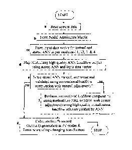
d. Map (Calculate) high quality and accuracy ANN Loadflow output data
set/vector (solution)
for a given input data set/vector using stored ANN.
e. If stored ANN trained, and tested and validated using conventional
loadflow computation
method like NRL or SSDL with control adjustments that accounts for physical
limits of
power network component equipments like reactive power generation limits of
generators,
and tap changing limits of tap changing transformers, go to step-g, or else
follow the next
step-f.
f. Perform conventional loadflow computation using method like NRL or SSDL
with control
adjustments using high quality initialization loadflow solution yielded by ANN
g. From calculated and known values of voltage magnitude and voltage angle
at different
power network nodes, and tap position of tap changing transformers, calculate
power flows
through power network components, and reactive power generation at PV-nodes.
Feature Selection Technique
[047] When an ANN is constructed and designed for single output
variable/parameter calculation
as in Fig. 5c, the total number of ANNs required for the unified functions of
loadflow computation
and contingency evaluations are 2(n-1) as there are two variables/parameters
are to be calculated
for each power network node. Similarly for steady state voltage and angle
stability calculations
combined, total number of ANNs required are 2m. The input vector for all these
[2(n-2) + 2m]
3/26/2014
CA 02712873 2014-03-26
ANNs is the same of dimension 2n, which is prohibitively large for power
networks of the order of
1000s of nodes. This is because the number of connection weights that must be
determined in the
training process increase with increasing number of input nodes. It will take
a long time to train the
ANN if there are a great number of inputs. In the worst case, the training
process may fail to
converge or may converge to local minimum that results in poor performance in
the testing and
validating phase. Therefore it is essential to reduce the number of inputs to
the ANN and retain
only those system variables that have significant effects on the desired or
target output. Feature
selection is especially important when we manage to apply ANN to a power
system containing a
great number of elements and variables. To train and finally store an ANN
capable of yielding
accurate estimates of voltage magnitudes, angles, V-stability index/margin,
and 0-stability
index/margin, it is essential to identify the key system features that affect
these stated variables the
most and employ the identified features as the inputs to the ANN. An approach
based on system
entropy is normally used as described in the available literature and in some
of the reference cited
in the above in this document. However, an invented approach is to use the
technique of Suresh's
diakoptics claimed in US Patent Number: 7788051 dated August 31, 2010: "Method
and
Apparatus for Parallel Loadflow Computation for Electric Power System". The
Suresh's diakoptics
technique determines a sub-network for each node involving directly connected
nodes referred to
as level-1 nodes and their directly connected nodes referred to as level-2
nodes and so on, wherein
the level of outward connectivity for a local sub-network around a given node
whose single
variable is to be estimated using separate ANN is to be determined
experimentally. For example,
an estimation of a node variable by a separate ANN for each variable in 1000
node power system
requires 2000 inputs. Whereas an invented approach stated in the above can
reduce required inputs
to about 200 by determining sub-network of may be say 5 to 20 levels of
outward connectivity
around a node whose single variable is to be estimated using the separate ANN.
1048] Fig. 6 is the overall integrated flow-chart of invented ANN Loadflow
based security
evaluation functions. Its separate steps are not elaborated and listed here
because they are self-
explanatory based on above description and publicly available literature.
Moreover, they do not
form part of claims.
26
3/26/2014
CA 02712873 2014-03-26
General Statements
[049] The system stores a representation of the reactive capability
characteristic of each machine
and these characteristics act as constraints on the reactive power, which can
be calculated for each
machine.
[050] While the description above refers to particular embodiments of the
present invention, it will
be understood that many modifications may be made without departing from the
spirit thereof. The
accompanying claims are intended to cover such modifications as would fall
within the true scope
and spirit of the present invention.
[051] The presently disclosed embodiments are therefore to be considered in
all respect as
illustrative and not restrictive, the scope of the invention being indicated
by the appended claims in
addition to the foregoing description, and all changes which come within the
meaning and range of
equivalency of the claims are therefore intended to be embraced therein.
27
3/26/2014