Note: Descriptions are shown in the official language in which they were submitted.
CA 02750255 2011-07-20
WO 2010/085497 PCT/US2010/021524
TITLE: TIME REVERSE IMAGING ATTRIBUTES
Background of the Disclosure
Technical Field
[0001] The disclosure is related to seismic exploration for oil and gas, and
more
particularly to determination of the positions of subsurface reservoirs.
Description
[0002] Geophysical and geological exploration investment for hydrocarbons is
often
focused on acquiring data in the most promising areas using relatively slow
methods,
such as reflection seismic data acquisition and processing. The acquired data
are used for
mapping potential hydrocarbon-bearing areas within a survey area to optimize
exploratory or production well locations and to minimize costly non-productive
wells.
[0003] The time from mineral discovery to production may be shortened if the
total
time required to evaluate and explore a survey area can be reduced by applying
geophysical methods alone or in combination. Some methods may be used as a
standalone decision tool for oil and gas development decisions when no other
data is
available.
[0004] Geophysical and geological methods are used to maximize production
after
reservoir discovery as well. Reservoirs are analyzed using time lapse surveys
(i.e. repeat
applications of geophysical methods over time) to understand reservoir changes
during
production. The process of exploring for and exploiting subsurface hydrocarbon
reservoirs is often costly and inefficient because operators have imperfect
information
from geophysical and geological characteristics about reservoir locations.
Furthermore, a
reservoir's characteristics may change as it is produced.
[0005] The impact of oil exploration methods on the environment may be reduced
by
using low-impact methods and/or by narrowing the scope of methods requiring an
active
source, including reflection seismic and electromagnetic surveying methods.
Various
geophysical data acquisition methods have a relatively low impact on field
survey areas.
Low-impact methods include gravity and magnetic surveys that maybe used to
enrich or
1
CA 02750255 2011-07-20
WO 2010/085497 PCT/US2010/021524
corroborate structural images and/or integrate with other geophysical data,
such as
reflection seismic data, to delineate hydrocarbon-bearing zones within
promising
formations and clarify ambiguities in lower quality data, e.g. where
geological or near-
surface conditions reduce the effectiveness of reflection seismic methods.
2
CA 02750255 2011-07-20
WO 2010/085497 PCT/US2010/021524
SUMMARY
[0006] A method and system for processing synchronous array seismic data
includes
acquiring synchronous passive seismic data from a plurality of sensors to
obtain
synchronized array measurements. A reverse-time data propagation process is
applied to
the synchronized array measurements to obtain a plurality of dynamic particle
parameters
associated with subsurface locations. Imaging conditions are applied to obtain
imaging
values that may be summed or stacked to obtain a time reverse image attribute.
A volume
of imaging values may be scaled by a non-signal noise function to obtain a
modified
image that is compensated for noise effects.
3
CA 02750255 2011-07-20
WO 2010/085497 PCT/US2010/021524
BRIEF DESCRIPTION OF THE DRAWINGS
Fig. 1 is a schematic illustration of a method according to an embodiment of
the present
disclosure for calculating a time reverse image attribute;
Fig. 2 illustrates various non-limiting possibilities for arrays of sensor for
data acquisition
of synchronous signals;
Fig. 3 is a flow chart of reverse-time processing for application to seismic
data;
Fig. 4 is a flow chart of a data processing flow that includes reverse-time
propagation
processing of field data;
Fig. 5 illustrates a flow chart of a reverse-time propagation process to
determine a time
reverse imaging attribute;
Fig. 6 illustrates a flow chart according to an embodiment of the present
disclosure for
determining a signal to noise image that includes executing a time reverse
image
processing method with acquired seismic data as input;
Fig. 7 illustrates a flow chart for determining an image domain stack
attribute;
Fig. 8 illustrates the output from a division of a `real' dataset with a
`random' dataset to
produce an image-domain signal to noise estimate;
Fig. 9 illustrates a 2-D profile result of summing imaging condition data
output along the
depth axis; and
Fig. 10 is diagrammatic representation of a machine in the form of a computer
system
within which a set of instructions, when executed may cause the machine to
perform any
one or more of the methods and processes described herein.
4
CA 02750255 2011-07-20
WO 2010/085497 PCT/US2010/021524
DETAILED DESCRIPTION
[0007] Information to determine the location of hydrocarbon reservoirs may be
extracted from naturally occurring seismic waves and vibrations measured at
the earth's
surface using passive seismic data acquisition methods. Seismic wave energy
emanating
from subsurface reservoirs, or otherwise altered by subsurface reservoirs, is
detected by
arrays of sensors and the energy back-propagated with reverse-time processing
methods
to locate the source of the energy disturbance. An imaging methodology for
locating
positions of subsurface reservoirs may be based on various time reversal
processing
algorithms of time series measurements of passive or active seismic data.
[0008] This disclosure teaches attributes extracted directly from energy
focused or
localized by the reverse time propagation. Additionally, this disclosure
teaches that
artificial or ambiguous focusing of reverse time images may be ameliorated or
removed
by accounting for the imaging artifacts velocity may introduce.
[0009] The methods disclosed here are equally applicable to seismic data
acquired
with so-called active or artificial sources or as part of a passive
acquisition program.
Passive seismic data acquisition methods rely on seismic energy from sources
not directly
associated with the data acquisition. In passive seismic monitoring there may
be no
actively controlled and triggered source. Examples of sources recorded that
may be
recorded with passive seismic acquisition are microseisms (e.g., rhythmically
and
persistently recurring low-energy earth tremors), microtremors and other
ambient or
localized seismic energy sources.
[0010] Microtremors are often attributed to the background energy normally
present
or occurring in the earth. Microtremor seismic waves may include sustained
seismic
signals within various or limited frequency ranges. Microtremor signals, like
all seismic
waves, contain information affecting spectral signature characteristics due to
the media or
environment that the seismic waves traverse as well as the source of the
seismic energy.
These naturally occurring, low amplitude and often relatively low frequency
background
seismic waves (sometimes termed noise or hum) of the earth may be generated
from a
variety of sources, some of which may be unknown or indeterminate.
CA 02750255 2011-07-20
WO 2010/085497 PCT/US2010/021524
[0011] Characteristics of microtremor seismic waves in the "infrasonic' range
may
contain relevant information for direct detection of subsurface properties
including the
detection of fluid reservoirs. The term infrasonic may refer to sound waves
below the
frequencies of sound audible to humans, and nominally includes frequencies
under 20
Hz.
[0012] Synchronous arrays of sensors are used to measure vertical and
horizontal
components of motion due to background seismic waves at multiple locations
within a
survey area. The sensors measure orthogonal components of motion
simultaneously.
[0013] Local acquisition conditions within a geophysical survey may affect
acquired
data results. Acquisition conditions impacting acquired signals may change
over time
and may be diurnal. Other acquisition conditions are related to the near
sensor
environment. These conditions may be accounted for during data reduction.
[0014] The sensor equipment for measuring seismic waves may be any type of
seismometer for measuring particle dynamics, such as particle displacements or
derivatives of displacements. Seismometer equipment having a large dynamic
range and
enhanced sensitivity compared with other transducers, particularly in low
frequency
ranges, may provide optimum results (e.g., multicomponent earthquake
seismometers or
equipment with similar capabilities). A number of commercially available
sensors
utilizing different technologies may be used, e.g. a balanced force feed-back
instrument
or an electrochemical sensor. An instrument with high sensitivity at very low
frequencies
and good coupling with the earth enhances the efficacy of the method. The data
measurements may be recorded as particle velocity values, particle
acceleration values or
particle pressure values.
[0015] Noise conditions representative of seismic waves that may have not
traversed
or been affected by subsurface reservoirs can negatively affect the recorded
data.
Techniques for removing unwanted noise and artifacts and artificial signals
from the data,
such as cultural and industrial noise, are important where ambient noise is
relatively high
compared with desired signal energy.
[0016] Time-reverse data propagation may be used to localize relatively weak
seismic events or energy, for example if a reservoir acts as an energy source,
an energy
6
CA 02750255 2011-07-20
WO 2010/085497 PCT/US2010/021524
scatterer or otherwise significantly affects acoustic energy traversing the
reservoir,
thereby allowing the reservoir to be located. The seismograms measured at a
synchronous
array of sensor stations are reversed in time and used as boundary values for
the reverse
processing. A time-reversed seismic wave field is injected into the earth
model at the
sensor position and propagated through the model. Various imaging conditions
may be
applied to enhance the processing that localizes the events or energy. Time-
reverse data
processing is able to localize event or energy sources with extremely low S/N-
ratios.
[0017] Field surveys have shown that hydrocarbon reservoirs may act as a
source of
low frequency seismic waves and these signals are sometimes termed
"hydrocarbon
microtremors." The frequency ranges of microtremors have been reported between
-1Hz
to 6Hz or greater. A direct and efficient detection of hydrocarbon reservoirs
is of central
interest for the development of new oil or gas fields. If there is a steady
source origin (or
other wave field alteration) of low-frequency seismic waves within a
reservoir, the
location of the reservoir may be located using time reverse propagation
combined with
the application of one or more imaging conditions. Time reverse propagation
may be
associated with wave field decomposition. The output of this processing can be
used to
locate and differentiate stacked reservoirs.
[0018] Time reverse propagation of acquired seismic data, which may be in
conjunction with modeling, using a grid of nodes is an effective tool to
detect the locality
of an origin of low-frequency seismic waves. As a non-limiting example for the
purposes
of illustration since microtremor characteristics are variable over time and
space, as well
as affected by subsurface structure and near surface conditions, microtremors
may
comprise low-frequency signals with a fundamental frequency of about 3Hz and a
range
between 1.5Hz and 4.5Hz. Hydrocarbon affected seismic data that include
microtremors
may have differing values that are reservoir or case specific. Processed data
images
representing one or more time steps showing a dynamic particle motion value
(e.g.,
displacement, velocity, acceleration or pressure) at every grid point may be
produced
during the reverse-time signal processing. Data for grid nodes or earth-model
areas
representing high or maximum particle velocity values may indicate the
location of a
specific source (or a location related to seismic energy source aberration) of
the forward
or field acquired data. The maximum dynamic particle parameters at model grid
nodes
7
CA 02750255 2011-07-20
WO 2010/085497 PCT/US2010/021524
obtained from the reverse-time data propagation may be used to delineate
parameters
associated with the subsurface reservoir location. Alternative imaging
conditions useful
with reverse time imaging of subsurface energy sources include combinations of
particle
dynamic behaviors and relationships, including phase and wave mode
relationships.
[0019] There are many known methods for a reverse-time data process for
seismic
wave field imaging with Earth parameters from acquired seismic data. For
example,
finite-difference, ray-tracing and pseudo-spectral computations, in two- and
three-
dimensional space, are used for full or partial wave field simulations and
imaging of
seismic data. Reverse-time propagation algorithms may be based on finite-
difference,
ray-tracing or pseudo-spectral wave field extrapolators. Output from these
reverse-time
data processing routines may include amplitudes for displacement, velocity,
acceleration
or pressures values at every time step of the imaging.
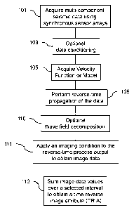
[0020] Fig. 1 illustrates a method according to a non-limiting embodiment of
the
present disclosure that includes acquiring seismic data to determine a
subsurface location
for hydrocarbons or other reservoir fluids. The embodiment, which may include
one or
more of the following (in any order), includes acquiring synchronous array
seismic data
having a plurality of components 101. The acquired data from each sensor
station may
be time stamped and include multiple data vectors. An example is passive
seismic data,
such as multicomponent seismometry data from long period sensors, although
"passive
acquisition" is not a requirement. The multiple data vectors may each be
associated with
an orthogonal direction of movement. The vector data may be arbitrarily mapped
or
assigned to any coordinate reference system, for example designated east,
north and
depth (e.g., respectively, Ve, Vn and Vz) or designated V,, Vy and Vz
according to any
desired convention and is amenable to any coordinate system.
[0021] The data may be optionally conditioned or cleaned as necessary 103 to
account for unwanted noise or signal interference. For example various
processing steps
such as offset removal, detrending the signal and band pass or other targeted
frequency
filtering or any other seismic data processing/conditioning methods as known
by
practitioners in the seismic arts. The vector data may be divided into
selected time
8
CA 02750255 2011-07-20
WO 2010/085497 PCT/US2010/021524
windows for processing. The length of time windows for analysis may be chosen
to
accommodate processing or operational concerns.
[0022] Additionally, signal analysis, filtering, and suppressing unwanted
signal
artifacts may be carried out efficiently using transforms applied to the
acquired data
signals. The data may be resampled to facilitate more efficient processing. If
a preferred
or known range of frequencies for which a hydrocarbon signature is known or
expected,
an optional frequency filter (e.g., zero phase, Fourier of other wavelet type)
may be
applied to condition the data for processing. Examples of basis functions for
filtering or
other processing operations include without limitation the classic Fourier
transform or
one of the many Continuous Wavelet Transforms (CWT) or Discrete Wavelet
Transforms. Examples of other transforms include Haar transforms, Haademard
transforms and Wavelet Transforms. The Morlet wavelet is an example of a
wavelet
transform that often may be beneficially applied to seismic data. Wavelet
transforms have
the attractive property that the corresponding expansion may be differentiable
term by
term when the seismic trace is smooth.
[0023] Imaging using field-acquired passive seismic data, or any seismic data,
to
determine the location of subsurface reservoirs includes using the acquired
time-series
data as `sources' in reverse-time wave propagation, which requires velocity
information
105. This velocity information may be a known function of position or
explicitly defined
with a velocity model. A reverse-time propagation of the data 109 is performed
by
injecting the time-reversed wave-field at the recording stations. The output
of the
reverse-time processing includes one or more measures of the dynamic particle
motion of
sources associated with subsurface positions (which may be nodes of
mathematical
descriptions (i.e., models) of the earth).
[0024] Optionally, wave equation decomposition 110 may be applied to the data
undergoing reverse time propagation to facilitate various imaging conditions
to apply to
the data. An imaging condition is applied to the dynamic particle motion
output during
the reverse-time processing 111. The final output of the reverse-time
processing depends
on the imaging condition or conditions used. Imaging conditions are developed
in more
detail below and include one or of: EE (x, t) = P (x, t) 2 = (/I + 2 ) (V = u
I t) 2, ES (x, t) _
9
CA 02750255 2011-07-20
WO 2010/085497 PCT/US2010/021524
S(x, t)2 = (-V x uIt)2, Ip(x) = Et P(x, t)P(x, t), IS(x) = EtS(x, t)S(x, t),
IPS(x) =
Zt P(x, t)S(x, t), and le (x) = Zt EE(x, t)ES(x, t). The imaging condition
output values
may be summed 113 over in interval, in depth or time, horizontally or
vertically, to aid in
the determination of the location of the energy source or the reservoir
location.
[0025] For the purposes of illustrating one embodiment of the time reverse
imaging
attribute (TRIA), selecting the maximum dynamic particle motion output at any
node
during the reverse time propagation is used as an example of an imaging
condition.
However, it will be appreciated that the TRIA is applicable for use with any
imaging
condition, including examples associated with wave-field decompositions
described later
herein. For this example, the maximum values derived from dynamic particle
motion,
which may be displacements, velocities or accelerations, may be collected to
determine
the energy source location contributing to the dynamics. Plotting the maximum
dynamic
values across all nodes may provide a basis for interpreting the location of a
subsurface
reservoir. A TRIA is determined 115 by summing the amplitude values along
selected
intervals in depth or time to indicate the position of a reservoir that is the
source of
hydrocarbon tremors. The data may be contoured or otherwise graphically
displayed to
illuminate reservoir positions.
[0026] Field data may be acquired with surface arrays, which may be 2D or 3D,
or
even arbitrarily positioned sensors 201 as illustrated in Fig. 2. Fig. 2
illustrates various
acquisition geometries which may be selected based on operational
considerations. Array
220 is an array for acquiring a 2D dataset (distance and time) and while
illustrated with
regularly spaced sensors 201, regular distribution is not a requirement. Array
230 and
240 are example illustrations of arrays for acquiring 3D datasets. Sensor
distribution 250
could be considered an array of arbitrarily placed sensors and may even
provide for some
modification of possible spatial aliasing that can occur with regular spaced
sensor 201
acquisition arrays.
[0027] While data may be acquired with multi-component earthquake seismometer
equipment with large dynamic range and enhanced sensitivity, many different
types of
sensor instruments can be used with different underlying technologies and
varying
sensitivities. Sensor positioning during recording may vary, e.g. sensors may
be
CA 02750255 2011-07-20
WO 2010/085497 PCT/US2010/021524
positioned on the ground, below the surface or in a borehole. The sensor may
be
positioned on a tripod or rock-pad. Sensors may be enclosed in a protective
housing for
ocean bottom placement. Wherever sensors are positioned, good coupling results
in
better data. Recording time may vary, e.g. from minutes to hours or days. In
general
terms, longer-term measurements may be helpful in areas where there is high
ambient
noise and provide extended periods of data with fewer noise problems.
[0028] The layout of a data survey may be varied, e.g. measurement locations
may be
close together or spaced widely apart and different locations may be occupied
for
acquiring measurements consecutively or simultaneously. Simultaneous recording
of a
plurality of locations (a sensor array) may provide for relative consistency
in
environmental conditions that may be helpful in ameliorating problematic or
localized
ambient noise not related to subsurface characteristics of interest.
Additionally the array
may provide signal differentiation advantages due to commonalities and
differences in
the recorded signal.
[0029] A non-limiting example of a reverse-time processing imaging is
illustrated in
Fig. 3 wherein seismic data are input 301 to the processing flow. The data may
optionally be filtered to a selected frequency range. A velocity model for the
reverse-
time process may be determined from known information 303 or estimated. A wave-
equation reverse-time imaging is performed 305 to obtain particle dynamic
behavior 307.
[0030] The reverse-time propagation process may include development of an
earth
model based on a priori knowledge or estimates of physical parameters of a
survey area
of interest. During data preparation, forward modeling may be useful for
anticipating and
accounting for known seismic signal or refining the velocity model or
functions used for
the reverse time processing. Modeling may include accounting for, or the
removal of, the
near sensor signal contributions due to environmental field effects and noise
and, thus,
the isolation of those parts of acquired data signals believed to be
associated with
environmental components being examined. By adapting or filtering the data
between
successive iterations in the imaging process, predicted signal can be
obtained, thus
allowing convergence to a structure element indicating whether a reservoir is
present
within the subsurface.
11
CA 02750255 2011-07-20
WO 2010/085497 PCT/US2010/021524
[0031] Time-reverse imaging (TRI) locates sources from acoustic, elastic, EM
or
optical measurements. It is the process of injecting a time reversed wave
field at the
recording locations and propagating the wave field through an earth model. A
TRM result
contains the complete time axis which an observer visually scans through to
locate
energetic focus locations (e.g., using velocity particle maxima). These focal
locations are
indicative of the constructive interference of energy at a source location.
[0032] However, rather than maintain the time axis, it can be collapsed by
applying
an imaging condition (IC) to produce a single image in physical space. The
chain of
operations of propagating a time-reversed wave field through a model and
applying an
imaging condition is referred to as time-reverse imaging (TRI).
[0033] When recording the ambient seismic wave field, multi-component sensors
are
placed at discrete locations. Therefore, when injecting the data into the
model domain,
point sources are created at recording locations. After sufficient propagation
steps, the
full wave field will be approximated. The depth at which the sampled wave
field
approximates the full wave field is a function of spatial sampling and the
velocity model
parameters, but is usually 1 to 1.5 times the spatial sampling.
[0034] From a multi-component data set, individual propagation modes are
extracted
from the full wave field. For the isotropic case, two vector identities are
required to
separate the P- and S- wave modes from the full displacement wave-field u(x,
t) at each
time step. For two-dimensional models x refers to the spatial dimensions (x,
z). Without
loss of generality, x can also refer to the 3-dimensional (x, y, z) case. The
wave field
decomposition step is inserted into the TRI algorithm before applying the
imaging
condition. Since the curl of the irrotational potential is zero and the
divergence of the
solenoidal potential is zero, the compressional, Ep(x, t), and shear, ES(x,
t), kinetic energy
densities are EP(x, t) = P(x, t)2 = ()L + 2 )(V = uI t)Z, and E, (x, t) = S(x,
t)2 =
(-V x uI t)2, where k and are the Lame coefficients. The derivatives are
evaluated at
each time step, t.
[0035] Separating the wave field allows for multiple imaging conditions to be
applied
based upon the expected source type. These imaging conditions are based on
extracting
the zero-lag of a cross-correlation along the time axis at every spatial
location. The
12
CA 02750255 2011-07-20
WO 2010/085497 PCT/US2010/021524
imaging conditions are the zero-lag of the P-wave autocorrelation, Ip, the
zero-lag of the
S-wave autocorrelation, I, the zero-lag of the P- and S-wave cross-
correlation, Ip, and
the zero-lag of the cross-correlation of the P- and S-wave energy densities,
Ie. These
imaging conditions are expressed as: Ip (x) = Z t P (x, t) P (x, t),
Is(x) = >t S(x, t)S(x, t), Is(x) = >t P(x, t)S(x, t), and Ie(x) _ >t Ep(x,
t)Es(x, t).
[0036] These image conditions, except for the cross-correlation of the P- and
S-
waves, have squared the wave field components, and thus produce non-negative
images.
The cross-correlation of the P- and S-waves has 0-mean, and has a zero-
crossing at the
source location, which is a function of the source type.
[0037] Fig. 4 illustrates an example of reverse-time imaging for locating an
energy
source or a reservoir in the subsurface using a velocity model 402 as input.
The reverse
time propagation may be wave equation based. Any available geoscience
information
401 may be used as input to determine parameters for an initial model 402 that
may be
modified as input to a reverse-time data propagation process 403 as more
information is
available or determined. Synchronously acquired passive seismic data 405 are
input
(after any optional processing/conditioning) to the reverse-time propagation
process 403.
Particle dynamics such as displacement, velocity or acceleration (or pressure)
are
determined from the processed data for determining dynamic particle behaviour
404. For
the data range processed for reverse time propagation, an imaging condition
406 is
applied. The imaging condition may be one or more of: EP (x, t) = P (x, t) 2 =
(A + 21i)(o = ul t)Z, ES(x, t) = S(x, t)2 = (-V x ult)2, Ip(x) _ Et P(x,
t)P(x, t),
Is(x) = Et S(x, t)S(x, t), Ips(x) = Et P(x, t)S(x, t), and Ie(x) _ Et Ep(x,
t)Es(x, t).
The output from the application of the imaging condition is stored or
displayed 410 to
determine subsurface reservoir positions. Alternatively, other imaging
conditions may be
applied, including imaging conditions determined for seismic data using wave
field
decomposition.
[0038] Fig. 5 illustrates an example of a reverse-time propagation process to
determine a time reverse imaging attribute (TRIA) useful for locating a
reservoir or
energy source in the subsurface using a velocity model 402 as input for a
reverse-time
imaging. The reverse time imaging may be wave equation based. Any available
13
CA 02750255 2011-07-20
WO 2010/085497 PCT/US2010/021524
geoscience information 401 may be used as input to determine parameters for an
initial
model 402 that may be modified as input to reverse-time data propagation 503
as more
information is available or determined. Synchronously acquired seismic data
405 are
input (after any optional processing/conditioning) to the reverse-time data
process 503.
One or more imaging conditions are applied to the time-reversed data to obtain
imaging
values 505 associated with subsurface locations. The imaging condition may be
one or
more of: Ep(x, t) = P(x, t) 2 = (/I + 2 )(V = u1 t)2, ES(x, t) = S(x, t)2 = (-
V x uI t)2,
Ip(x) = Et P(x, t)P(x, t), IS(x) = EtS(x, t)S(x, t), IPS(x) = Et P(x, t)S(x,
t), and
le (x) = Zt EE (x, t) ES (x, t). The imaging values may optionally be stored
or displayed
506. These output values, which depending on the selected imaging condition
may be
proportional to energy, are representative over the subsurface volume of the
energy that
has originated from the associated subsurface location. TRIA is obtained for a
selected
interval (in time or depth) by summing the values over the selected interval
507. The
TRIA may be projected to the earth surface or a subsurface horizon in
association with a
surface sensor position or any arbitrary position to provide an indication of
areal extent of
a subsurface energy source anomaly or hydrocarbon reservoir. The TRIA may be
stored
or displayed 512.
[0039] An example of an embodiment illustrated here uses a numerical modeling
algorithm similar to a rotated staggered grid finite-difference technique. The
two
dimensional numerical grid is rectangular. Computations may be performed with
second
order spatial explicit finite difference operators and with a second order
time update.
However, as will be well known by practitioners familiar with the art, many
different
reverse-time methods may be used along with various wave equation approaches.
Extending methods to three dimensions is straightforward.
[0040] In one non-limiting embodiment a method and system for processing
synchronous array seismic data includes acquiring synchronous passive seismic
data from
a plurality of sensors to obtain synchronized array measurements. A reverse-
time data
propagation process is applied to the synchronized array measurements to
obtain a
plurality of dynamic particle parameters associated with subsurface locations.
These
dynamic particle parameters are stored in a form for display. Maximum values
of the
14
CA 02750255 2011-07-20
WO 2010/085497 PCT/US2010/021524
dynamic particle parameters may be interpreted as reservoir locations. The
dynamic
particle parameters may be particle displacement values, particle velocity
values, particle
acceleration values or particle pressure values. The sensors may be three-
component
sensors. Zero-phase frequency filtering of different ranges of interest may be
applied.
The data may be resampled to facilitate efficient data processing.
[0041] A system response is the convolution of a seismic signal with a
velocity
model. Different velocity models engender different responses to the same
seismic input.
Particular models may have system responses that obscure the source locations
even with
high signal to noise ratios. An example is the "ringing" in low velocity
layers. The
system response to field data will contain contributions from signal, noise
and sampling
artifacts. To accurately interpret the signal contribution, it is important to
estimate and
remove the any portion of a system response to non-signal components. A non-
signal
noise data set may be used to remove non-signal contributions to a system
response.
[0042] A non-signal noise-dataset may be developed from noise traces from an
appropriate noise model containing seismic data scaled to the amplitude and
frequency
band of the acquired field data. This ensures that the noise traces have equal
energy to the
recorded traces but without any correlated phase information. The advantage of
this type
of noise model is that it is based directly on the data. No information about
the
acquisition environment is necessary. The noise model seismic data may be
generated
from random input or forward modeling.
[0043] Once created, the non-signal noise-dataset is imaged with the TRI
algorithm
in the same fashion with the same velocity field as the field seismic data.
This synthetic
image derived using the velocity field will estimate the system response to
both the non-
signal noise-dataset and sampling artifacts. In this way, it is possible to
create an
estimate of the signal to noise ratio in the image domain. The recorded data,
d, is a
combination of signal and noise: d = s + n. The image created from this data
is the
apparent signal image, S. Using capital letters to indicate images as a
function of space,
eg S(x) and lower case letters for recordings that functions of space and
time, eg d(x, t),
the apparent signal for the recorded data is defined as: S = Zt(st + nt)2 = Zt
st +
2stnt + nt, where the time-axis is summed over t. Dropping the subscript, the
estimated
CA 02750255 2011-07-20
WO 2010/085497 PCT/US2010/021524
noise image, N, is N = n2, where n is the noise data. The estimated signal
image, S, is
S=S - N.
[0044] A signal to noise estimate may be obtained by dividing the apparent
signal by
z
the noise estimate. The estimated signal to noise image is N + 1 = S = nz + 2
+
nz
z z
E nz . For noise estimated correctly, n n and Y_ nz 1. Therefore, the division
of
dataset S with dataset N results in an estimated signal to noise image.
[0045] Fig. 6 illustrates a flow chart according to an embodiment of the
present
disclosure for determining a noise domain signal to noise image estimate that
includes
executing a time reverse image processing method with acquired seismic data
601 as
input. The method includes estimating or compensating for the signal to noise
ratio in the
image domain. The process includes two essentially parallel processes
including the
input of a non-signal noise dataset 603 containing a substantially equivalent
amount of
energy and frequency content as the acquired seismic data 601 at each sensor
or
acquisition station for all components. The non-signal noise dataset may be
developed
from substantially random data or a forward modeling process may be used to
determine
the non-signal noise dataset if parameters are available. When both the real
seismic data
601 and non-signal 603 data are processed through to an imaging condition
result, the
images are divided or otherwise compared (e.g., Real image output divided by
the non-
signal image output) or otherwise processed together to determine where energy
originating in the subsurface focuses 625.
[0046] Following a reverse time propagation process similar to Fig. 4, the
synchronously acquired seismic array data 601 may be optionally filtered 605
or
otherwise processed to remove transients and noise. A scaling value (e.g. an
RMS value
determined from the seismic data) is calculated 609 that may also be used as
an input
parameter (611) for the nonsignal noise dataset sequence processing. Reverse
time
propagation (which may be referred to as acausal elastic propagation) is
applied to the
data 613 (e.g., Fig. 4). Acausal propagation of the data, or causal
propagation of time-
reversed data, will position the data through time to the location of the
source.
16
CA 02750255 2011-07-20
WO 2010/085497 PCT/US2010/021524
[0047] Optionally, the wavefield may be decomposed 617 so that one or more of
the
imaging conditions referred to above 621, for example an imaging condition
arbitrarily
designated "A" that may be one or more of IP, Is, IPS and/or Ie.
[0048] Random input seismic data 603 undergoes a similar processing sequence.
The
data may be optionally filtered 607 in the same or equivalent manner to 605
and may be
scaled 611 by the RMS or other scaling value calculated at 609. The data are
propagated
through the velocity model 615, as in 613, and the wavefield decomposed 619.
An
imaging condition "B" (that may be imaging condition "A") is applied to the
decomposed
data. After application of the selected imaging condition the output is an
apparent signal
image 622 or an estimated noise image 624. The estimated noise image 624,
generated
from the non-signal noise dataset, may optionally be smoothed. The data
determined at
622 and 624 may then be divided or otherwise scaled, for example the data
output from
622 may be divided by the data output from 624, which results in a signal to
noise image
625. This signal to noise image 625 may be considered as the effective removal
of an
image system response related to the velocity model.
[0049] Another embodiment according to the present disclosure comprises an
image
domain stack: After TRM or TRI processing, the image data or dynamic particle
values
are stacked vertically in time or depth to obtain a TRI attribute (TRIA). The
stacking
may be over a selected interval of interest or substantially the entire
vertical depth or time
range of the time reverse imaging. This attribute may be displayed in map form
over the
area of the seismic data acquisition, which results in the TRIA projected to
the surface.
This gives a surface map of where the energy is accumulating over the survey
area. The
data values projected to the surface may be contoured or otherwise processed
for display.
In some circumstances (for example sparse spatial sampling resulting in strong
apparent
near surface effects) it may be best to exclude the near surface from the TRIA
determination.
[0050] Fig. 7 illustrates that data processed to Imaging Condition "C" 721
that may,
for example, be an imaging condition applied to a decomposed wavefield of
acquired
seismic data may then be summed 707 along the depth or time axis.
Alternatively, the
imaging condition (IC) output may be summed along a horizontal interval or a
known
17
CA 02750255 2011-07-20
WO 2010/085497 PCT/US2010/021524
horizon interval. Imaging Condition "D" 723, applied to a non-signal noise
dataset,
which imaging condition may be equivalent to 721, but for a non-signal noise
dataset or a
time separated dataset may be combined with data from 721 at 725 to remove the
impulse
response prior to stacking along the depth axis 709. The data from 723 may
also be
summed 711 (as in 707) for comparison as well. These output values may also be
projected to the surface and contoured.
[0051] Fig. 8 illustrates a signal to noise image, or an image-domain signal
to noise
estimate, an example of the output of 625, the output of the division of a
`real' dataset
using field acquired seismic data, for example at step 622, by a dataset from
the same
location using the non-signal noise dataset input processed to an imaging
condition
representing an estimate of the noise, for example like 624 of Fig. 6. The
advantage is
that energy that may appear to focus in parts of the depth model is accounted
for since the
enhanced focus of random energy is accounted for in the output of this
processing.
[0052] Fig. 9 illustrates an example of the TRIA over a surface profile
obtained by
stacking the data (arbitrary vertical axis units) from the imaging condition
result along
the vertical axis (depth in this case) of the processing illustrated in Fig.
8. In this case the
near surface is not included since the numerical artifacts due to the
relatively sparse near
surface spatial sampling are strong and do not apparently contain accurate
information.
Alternatively, the data may be stacked or summed horizontally or along or in
depth or
time horizons.
[0053] Fig. 10 is illustrative of a computing system and operating environment
300
for implementing a general purpose computing device in the form of a computer
10.
Computer 10 includes a processing unit 11 that may include `onboard'
instructions 12.
Computer 10 has a system memory 20 attached to a system bus 40 that
operatively
couples various system components including system memory 20 to processing
unit 11.
The system bus 40 may be any of several types of bus structures using any of a
variety of
bus architectures as are known in the art.
[0054] While one processing unit 11 is illustrated in Fig. 10, there may be a
single
central-processing unit (CPU) or a graphics processing unit (GPU), or both or
a plurality
18
CA 02750255 2011-07-20
WO 2010/085497 PCT/US2010/021524
of processing units. Computer 10 may be a standalone computer, a distributed
computer,
or any other type of computer.
[0055] System memory 20 includes read only memory (ROM) 21 with a basic
input/output system (BIOS) 22 containing the basic routines that help to
transfer
information between elements within the computer 10, such as during start-up.
System
memory 20 of computer 10 further includes random access memory (RAM) 23 that
may
include an operating system (OS) 24, an application program 25 and data 26.
[0056] Computer 10 may include a disk drive 30 to enable reading from and
writing
to an associated computer or machine readable medium 31. Computer readable
media 31
includes application programs 32 and program data 33.
[0057] For example, computer readable medium 31 may include programs to
process
seismic data, which may be stored as program data 33, according to the methods
disclosed herein. The application program 32 associated with the computer
readable
medium 31 includes at least one application interface for receiving and/or
processing
program data 33. The program data 33 may include seismic data acquired
according to
embodiments disclosed herein. At least one application interface may be
associated with
applying an imaging condition and summing the image values along an interval
for
locating subsurface hydrocarbon reservoirs or energy sources.
[0058] The disk drive may be a hard disk drive for a hard drive (e.g.,
magnetic disk)
or a drive for a magnetic disk drive for reading from or writing to a
removable magnetic
media, or an optical disk drive for reading from or writing to a removable
optical disk
such as a CD ROM, DVD or other optical media.
[0059] Disk drive 30, whether a hard disk drive, magnetic disk drive or
optical disk
drive is connected to the system bus 40 by a disk drive interface (not shown).
The drive
30 and associated computer-readable media 31 enable nonvolatile storage and
retrieval
for application programs 32 and data 33 that include computer-readable
instructions, data
structures, program modules and other data for the computer 10. Any type of
computer-
readable media that can store data accessible by a computer, including but not
limited to
cassettes, flash memory, digital video disks in all formats, random access
memories
19
CA 02750255 2011-07-20
WO 2010/085497 PCT/US2010/021524
(RAMs), read only memories (ROMs), may be used in a computer 10 operating
environment.
[0060] Data input and output devices may be connected to the processing unit
11
through a serial interface 50 that is coupled to the system bus. Serial
interface 50 may a
universal serial bus (USB). A user may enter commands or data into computer 10
through input devices connected to serial interface 50 such as a keyboard 53
and pointing
device (mouse) 52. Other peripheral input/output devices 54 may include
without
limitation a microphone, joystick, game pad, satellite dish, scanner or fax,
speakers,
wireless transducer, etc. Other interfaces (not shown) that may be connected
to bus 40 to
enable input/output to computer 10 include a parallel port or a game port.
Computers
often include other peripheral input/output devices 54 that may be connected
with serial
interface 50 such as a machine readable media 55 (e.g., a memory stick), a
printer 56 and
a data sensor 57. A seismic sensor or seismometer for practicing embodiments
disclosed
herein is a nonlimiting example of data sensor 57. A video display 72 (e.g., a
liquid
crystal display (LCD), a flat panel, a solid state display, or a cathode ray
tube (CRT)) or
other type of output display device may also be connected to the system bus 40
via an
interface, such as a video adapter 70. A map display created from spectral
ratio values as
disclosed herein may be displayed with video display 72.
[0061] A computer 10 may operate in a networked environment using logical
connections to one or more remote computers. These logical connections are
achieved by
a communication device associated with computer 10. A remote computer may be
another computer, a server, a router, a network computer, a workstation, a
client, a peer
device or other common network node, and typically includes many or all of the
elements
described relative to computer 10. The logical connections depicted in Fig. 10
include a
local-area network (LAN) or a wide-area network (WAN) 90. However, the
designation
of such networking environments, whether LAN or WAN, is often arbitrary as the
functionalities may be substantially similar. These networks are common in
offices,
enterprise-wide computer networks, intranets and the Internet.
[0062] When used in a networking environment, the computer 10 may be connected
to a network 90 through a network interface or adapter 60. Alternatively
computer 10
CA 02750255 2011-07-20
WO 2010/085497 PCT/US2010/021524
may include a modem 51 or any other type of communications device for
establishing
communications over the network 90, such as the Internet. Modem 51, which may
be
internal or external, may be connected to the system bus 40 via the serial
interface 50.
[0063] In a networked deployment computer 10 may operate in the capacity of a
server or a client user machine in server-client user network environment, or
as a peer
machine in a peer-to-peer (or distributed) network environment. In a networked
environment, program modules associated with computer 10, or portions thereof,
may be
stored in a remote memory storage device. The network connections
schematically
illustrated are for example only and other communications devices for
establishing a
communications link between computers may be used.
[0064] In one nonlimiting embodiment a method for processing synchronous array
seismic data comprises acquiring seismic data from a plurality of sensors to
obtain
synchronized array measurements, applying a reverse-time data propagation
process to
the synchronized array measurements to obtain dynamic particle parameters
associated
with subsurface locations, applying an imaging condition, using a processing
unit, to the
dynamic particle parameters to obtain imaging values associated with
subsurface
locations and summing the imaging values over a selected interval to obtain a
time
reverse image attribute.
[0065] Another aspect includes storing the time reverse image attribute in a
form for
display.
[0066] Still another aspect includes selecting synchronized array measurements
for input
to the reverse-time data propagation process without reference to phase
information of
the seismic data. In another aspect the synchronized array measurements
comprises are
at least one selected from the group consisting of i) particle velocity
measurements, ii)
particle acceleration measurements, iii) particle pressure measurements and
iv) particle
displacement measurements. The plurality of sensors may be three-component
sensors.
[0067] In another aspect the time reverse image attribute may be scaled over
the selected
interval by a summed synthetic time reverse image attribute determined by
applying the
reverse time data process to synthetic seismic data, applying the imaging
condition to the
output of the reverse time data process and summing the synthetic imaging
values over
21
CA 02750255 2011-07-20
WO 2010/085497 PCT/US2010/021524
the selected interval. The method may further comprise applying a zero-phase
frequency
filter to the synchronized array measurements.
[0068] In another nonlimiting embodiment a set of application program
interfaces
embodied on a computer readable medium for execution on a processor in
conjunction
with an application program for applying a reverse-time data process to
synchronized
seismic data array measurements to obtain a time reverse image attribute
associated with
subsurface reservoir locations comprises a first interface that receives
synchronized
seismic data array measurements, a second interface that receives a plurality
of dynamic
particle parameters associated with a subsurface location, the parameters
output from
reverse-time data processing of the synchronized seismic data array
measurements, a
third interface that receives instruction data for applying an imaging
condition to the
dynamic particle parameters and a fourth interface that receives instruction
data for
summing output of the applied imaging condition along a selected interval to
obtain a
time reverse image attribute.
[0069] In another aspect the set of application interface programs further
comprises a
display interface that receives instruction data for displaying imaging-
condition
processed values of the plurality of dynamic particle parameters. Still
another aspect
comprises a velocity-model interface that receives instruction data for
reverse-time
propagation using a velocity structure associated with the synchronized
seismic data
array measurements. Yet another aspect of the set of application interface
programs
comprises a migration-extrapolator interface that receives instruction data
for including
an extrapolator for at least one selected from the group of i) finite-
difference time reverse
migration, ii) ray-tracing reverse time migration and iii) pseudo-spectral
reverse time
migration. Another aspect comprises an imaging-condition interface that
receives
instruction data for applying an imaging condition to dynamic particle
parameters output
from reverse-time data processing of synthetic seismic data array measurements
to obtain
synthetic image values. Another aspect of the application interface programs
comprises
an attribute-scaling interface that receives instruction data for scaling the
time reverse
image attribute by a function of a value determined by summing the synthetic
image
values along the selected interval. In still another aspect the set of
application interface
programs comprises a seismic-data-input interface that receives instruction
data for the
22
CA 02750255 2011-07-20
WO 2010/085497 PCT/US2010/021524
input of the plurality of seismic data array measurements that are at least
one selected
from the group consisting of i) particle velocity measurements, and ii)
particle
acceleration measurements and iii) particle pressure measurements.
[0070] In still another nonlimiting embodiment an information handling system
for
determining a time reverse image attribute for determinig the presence of
subsurface
hydrocarbons associated with an area of seismic data acquisition comprises a
processor
configured for applying a reverse-time data process to synchronized array
measurements
of seismic data to obtain dynamic particle parameters associated with
subsurface
locations, a processor configured for summing imaging values obtained from
applying an
imaging condition to the dynamic particle parameters associated with
subsurface
locations, the values summed along an interval to obtain a time-reversed-model-
attribute
and a computer readable medium for storing the time-reversed-model-attribute.
[0071] Another aspect of the information handling system is wherein the
processor is
configured to apply the reverse-time data process with a velocity model
comprising
predetermined subsurface velocity information associated with subsurface
locations. And
another aspect comprises a display device for displaying the dynamic particle
parameters.
Still another aspect involves the information handling system wherein the time-
reversed-
model-attribute is an output value from an imaging condition applied to the
plurality of
dynamic particle parameters. The processor of the information handling system
of may
be configured to apply the reverse-time data process with an extrapolator for
at least one
selected from the group of i) finite-difference reverse time migration, ii)
ray-tracing
reverse time migration and iii) pseudo-spectral reverse time migration. And
the
information handling system may further comprise a graphical display coupled
to the
processor and configured to present a view of the time-reversed-model-
attribute as a
function of position, wherein the processor is configured to generate the view
by
contouring values of the time-reversed-model-attribute over an area associated
with the
seismic data.
[0072] While various embodiments have been shown and described, various
modifications and substitutions may be made thereto without departing from the
spirit
and scope of the disclosure herein. Accordingly, it is to be understood that
the present
embodiments have been described by way of illustration and not limitation.
23