Note: Descriptions are shown in the official language in which they were submitted.
X-RAY REDUCTION SYSTEM
FIELD
The invention is related to the field of multiple frame x-ray imaging and more
particularly to the field of controlling x-ray radiation amount during
multiple frame
x-ray imaging.
BACKGROUND
In a typical multiple frame x-ray imaging system the x-ray tube generates x-
ray
radiation over a relatively wide solid angle. To avoid unnecessary exposure to
both the patient and the medical team, collimators of x-ray absorbing
materials
such as lead are used to block the redundant radiation. This way only the
necessary solid angle of useful radiation exits the x-ray tube to expose only
the
necessary elements.
Such collimators are used typically in a static mode but may assume a variety
of
designs and x-ray radiation geometry. Collimators can be set up manually or
automatically using as input, for example, the dimensions of the organ
environment that is involved in the procedure.
In multiple frame x-ray imaging the situation is more dynamic than in a single
exposure x-ray. The x-ray radiation is active for relatively long period and
the
treating physician typically has to stand near the patient, therefore near the
x-ray
radiation. As a result, it is desired to provide methods to minimize exposure
to
the medical team. Methods for reducing x-ray radiation intensity have been
suggested where the resultant reduced signal to noise ratio (S/11) of the x-
ray
image in compensated by digital image enhancement. Other methods suggest a
collimator limiting the solid angle of the x-ray radiation to a fraction of
the image
intensifier area and moving the collimator to swap the entire input area of
the
1
CA 2893671 2018-11-30
image intensifier where the Region of Interest (ROI) is exposed more than the
rest of the area. This way, the ROI gets high enough x-ray radiation to
generate a
good SIN image while the rest of the image is exposed with low x-ray
intensity,
providing a relatively low SIN image. The ROI size and position can be
determined in a plurality of methods. For example, it can be a fixed area in
the
center of the image or it can be centered automatically about the most active
area in the image, this activity is determined by temporal image analysis of s
sequence of cine images received from the video camera of the multiple frame x-
ray imaging system.
SUMMARY
According to a first aspect of the present invention there is provided an x-
ray
system incorporating an x-ray source, a detector, a monitor for displaying an
x-
ray image of a field of view and an eye tracker wherein said eye tracker is
configured to provide user's gazing coordinates in the image area; said system
configured to determine a Region of Interest (ROI) so that the gazing point is
contained in said ROI; and to optimize the image displayed on said monitor
according to the image part that is contained in said ROI.
.. The image optimization may be made by controlling any of the following
parameters: x-ray tube current (whether in continuous or pulse modes); x-ray
tube Peak Kilo Voltage (PKV); x-ray pulse length; AGC (Automatic Gain
Control),
whether analog or digital; Tone reproduction of the image implemented in
brightness function; Tone reproduction of the image implemented in contrast
function; Tone reproduction of the image implemented in brightness function;
Tone reproduction of the image implemented in gamma function; Tone
reproduction of the image implemented in offset function; Tone reproduction of
the image implemented in n-degree linear function; and Tone reproduction of
the
image implemented in a non-linear function.
2
CA 2893671 2018-11-30
The x-ray system may further include a collimator, which may be configured to
modify the x-ray radiation dose per pixel (DPP) in the field of view according
to
the location of the gazing point.
The x-ray system may further include a collimator, which may be configured to
modify the dose per pixel (DPP) in the field of view according to the location
of
the gazing point.
According to a second aspect of the present invention there is provided an x-
ray
system incorporating an x-ray source, a detector, a monitor for displaying an
x-
ray image and a collimator; said collimator is configured to expose a first
area to
a first radiation level and a second area to a second radiation level; and
said
system configured to process said second area to become similar to said first
area using a tone-correction function.
The tone-correction functions may be one of at least two tone-correction
functions, each of the tone-correction functions is associated with a specific
PKV.
The system may further be configured to create a tone-correction function by
interpolation of two other tone-correction functions, each of the other tone-
correction functions associated with a specific PKV.
The system may further be configured to estimate a tone-correction function
for
a third area from the tone-correction function used for said second area.
The estimation may use exponential calculation.
The system may further be configured to adjust the input scale of the tone-
correction function to fit changes in x-ray current.
The adjustment may be made using a factor equal to the relative change of the
x-
ray current.
3
CA 2893671 2018-11-30
According to a third aspect of the present invention there is provided a
method of
calculating a tone-correction function including: exposing a first area to a
first x-
ray radiation and a second area to a second x-ray radiation, wherein at least
a
part of said first and second radiation is through a variable absorption
phantom
so that for each designated transmission level of said phantom there is at
least
one area exposed by said first radiation and at least one area exposed by said
second radiation; for each such designated transmission level calculating the
average pixel value; calculating the ratio of said two average pixel values
for all
designated absorption levels; and fitting a function to the said calculated
ratios to
be used as the tone-correction function.
The variable absorption phantom may be a step wedge.
.. The variable absorption phantom may be a variable thickness phantom of
continuous slope function.
According to a fourth aspect of the present invention there is provided a
method
of calculating a tone-correction function including: exposing an area to a
first x-
ray radiation and exposing said area to a second x-ray radiation, wherein said
first and second radiation is through a human tissue in said area; calculating
the
ratio of at least one pixel value in said area corresponding to said first
radiation to
the corresponding pixel value in said area corresponding to said second
radiation; and fitting a function to the said at least one calculated ratio
and pixel
value in said area corresponding to said second radiation to be used as a
first
tone-correction function. More than one area may be used.
A second tone-correction function may calculated, using also data that was
acquired after the acquisition of the data used to calculate said first tone-
correction function.
4
CA 2893671 2018-11-30
The data used to calculate said first tone-correction function may be from at
least
2 patients.
According to a fifth aspect of the present invention there is provided an x-
ray
system incorporating an x-ray source, a collimator, a detector and a monitor,
means for moving said collimator in a plane generally parallel to the plane of
said
collimator; said collimator comprising an aperture that allows all the
radiation to
pass through, an outer annulus that reduces the radiation passing through at
an
amount depending on the material and the thickness of the said outer annulus
and an inner annulus between said aperture and said outer annulus, with
thickness changing as a function of the distance from the said aperture,
starting
at a low thickness on the side of the aperture and ending at the thickness of
the
outer annulus on the side of the outer annulus; and the system configured to
modify image data so as to essentially adjust the image acquired through the
inner annulus and the image acquired through the outer annulus to appear
visually similar to the image acquired through said aperture, wherein
parameters
used for said adjustments depend on the position of said collimator.
The system may be configured to acquire said parameters by a calibration
procedure, said calibration procedure includes measurements made at a variety
of said collimator positions. The variety of collimator positions may include
a
variety of positions in the collimator plane. The variety of collimator
positions may
include a variety of distances from the x-ray source.
The internal annulus thickness may be essentially symmetrical relative to a
plane
that is located essentially midway between the two external surfaces of said
outer annulus.
The system may include a layer of material that is different from the material
of
the outer annulus, said layer located at said aperture area. The layer may
overlap at least a part of said inner annulus.
5
CA 2893671 2018-11-30
According to a sixth aspect of the present invention there is provided an x-
ray
system incorporating an x-ray source, a detector, a monitor for displaying an
x-
ray image, a collimator and an input device; wherein said input device is
-- configured to provide coordinates relative to the x-ray image; the system
configured to select a region of the image according to said coordinates; and
adjust at least one of the following parameters according to said coordinates:
said region shape; and said region position.
The system may further be configured to adjust at least one of the following
parameters according to said region: x-ray tube mA; x-ray tube mAs; x-ray tube
KVp; said x-ray image brightness; said image contrast; and said image tone.
The input device may be at least one of: an eye tracker; a joy-stick; a
keyboard;
an interactive display, a gesture reading device; and a voice interpreter.
BRIEF DESCRIPTION OF THE DRAWINGS
The invention will be better understood in reference to the following Figures:
Figure 1A is a simplified schematic illustration of an example layout of a
multiple
frame x-ray imaging clinical environment and system;
Figure 1 B is an illustration of an example of a layout of the system of
Figure 1A
showing additional details of components of the system example of the
invention;
Figure 2 is a schematic illustration of an example of image displayed on a
monitor of a multiple frame x-ray imaging system;
Figure 3 is a schematic illustration of additional aspects of the system
example of
Figure 1A;
6
CA 2893671 2018-11-30
Figure 4 is a schematic illustration of an example of x-ray exposure regions
of the
detector in reference to the parameters of Figure 3;
Figure 5 is a schematic illustration of an example of a collimator according
to the
8 present invention;
Figure 6 is a schematic illustration of an example of the exposed region of
the
image intensifier at a certain rotation angle of the collimator of Figure 5;
Figure 7 is a schematic illustration of an example of the light exposure
pattern of
the sensor at a certain rotation angle of the collimator of Figure 5;
Figure 8 is a schematic illustration of an example of reading process of pixel
values of the sensor.;
Figure 9 is a schematic illustration of an example of reading process of pixel
values of the sensor;
Figure 10A is a schematic illustration of a top view of an example of a
collimator
of the invention;
Figure 10B is a schematic illustration of a bottom view of the example
collimator
of Figure 10A;
Figure 100 is a schematic illustration of a cross-section view of the example
collimator of Figure 10A;
Figure 11A is a schematic illustration of the main parts of another example of
a
collimator of the invention;
7
CA 2893671 2018-11-30
Figure 11B is a schematic illustration of the parts of Figure 11A in the
operative
configuration;
Figure 11C is a schematic illustration of a cross section of Figure 11B;
Figure 11D is a schematic illustration of parts of the collimator example of
Figure
11B;
Figure 12A is a schematic illustration of the main modules of another example
of
a collimator of the invention;
Figure 12B is a schematic illustration of the modules of Figure 12A in the
operative configuration;
Figure 13A is a schematic illustration of another example of a collimator of
the
invention;
Figure 13B is a schematic illustration of another example of a collimator of
the
invention;
Figure 14A is a schematic illustration of the main parts of another example of
a
collimator of the invention;
Figure 14B is a schematic illustration of the parts of Figure 14A in the
operative
configuration;
Figure 15 is a schematic illustration of another 4 example of another
collimator of
the invention and a qualitative exposure generated by the collimator as a
distance from the center of rotation;
8
CA 2893671 2018-11-30
Figure 16 is a schematic illustration of another 4 example of another
collimator of
the invention;
Figure 17A is a schematic illustration of an example of ROI that is not
generally
located around the center of rotation;
Figure 17B is a schematic illustration of an example of changing the rotation
speed profile of a collimator to enhance the image quality of the ROI of
Figure
17A;
Figure 18 is a schematic illustration of an example of a non rotating
collimator
and the effect it has on an image displayed on the monitor;
Figure 19 is an example of the ROI of Figure 17A and a collimator that can be
displaced to bring the center of rotation to generally the center of the ROI;
Figure 20A is the same collimator example of Figure 5 provided here for visual
comparison with the collimator of Figure 20B;
Figure 20B is an example of a version of the collimator of Figure 5 with
larger
diameter and longer sector hole, used to avoid image shadowing during
displacement of the collimator;
Figure 21A presents a typical step wedge phantom for use with x-ray;
Figure 21B demonstrates different absorption in ROI and background areas due
to background filter and change in x-ray spectrum;
Figure 21C is an example of a tone-correction function made to tone-correct
the
background image to fit the ROI image;
9
CA 2893671 2018-11-30
Figure 21D is an example of a tone-correction function adjusted for x2 x-ray
exposure comparing to the x-ray exposure in the calculation stage;
Figure 21E is an enlargement of the function of Figure 21D, in the usable
range;
Figure 22A provides an illustration of an ROI location and background for
calculation of tone-correction function;
Figure 22B provides an illustration of another ROI location and background for
calculation of tone-correction function;
Figure 23A illustrates the path of two x-ray rays through the collimator of
Figure
18 at one collimator position;
Figure 23B illustrates the path of two x-ray rays through the collimator of
Figure
18 at a second collimator position;
Figure 24A illustrates the path of two x-ray rays through a collimator with
symmetric aperture edge at one collimator position;
Figure 243 illustrates the path of two x-ray rays through a collimator with
symmetric aperture edge at a second collimator position;
Figure 25 illustrates a modified example of collimator of Figure 18;
Figure 26 is a simplified schematic illustration of an example layout of a
multiple
frame x-ray imaging clinical environment and system with the addition of an
eye
tracker;
Figure 27 is a flowchart referencing Figure 1A, describing the basic multiple
frame x-ray imaging process using an eye tracker;
CA 2893671 2018-11-30
Figure 28A is a flowchart describing a method for displaying the complete data
from one EC using multiple frames, performing normalization on each frame
separately;
Figure 28B is a flowchart describing a method for displaying the complete data
from one EC using multiple frames, performing normalization after the frames
have been summed;
Figure 28C is a flowchart describing a method for displaying the complete data
from one EC using multiple frames, updating the display after every frame;
Figure 29 is a flowchart referencing Figure 8, describing the process of
reading
pixel values of the sensor;
Figure 30 is a flowchart referencing Figure 17B, describing the change in
rotation
speed profile of a collimator to incorporate an ROI that is not in the center
of the
display;
Figure 31 is a flowchart referencing Figure 18D, describing the adjustments
necessary to achieve homogenous SIN across variable collimator annulus
widths;
Figure 32 is a flowchart describing a method for gradually shifting the
display for
an image region previously in the ROI that has moved into the background;
Figure 33A is a flowchart referencing Figures 21A, 21B, 21C, describing the
process of generating a tone correction function using a variable absorption
phantom (VAP);
Figure 33B is a flowchart referencing Figures 22A, 22B, describing the process
of
generating a tone correction function using the patient's body;
11
CA 2893671 2018-11-30
Figure 34A is a schematic diagram of an x-ray system with a detector utilized
with different zoom levels;
Figure 34B is a diagram of an example of a collimator with 3 ROI elements;
Figure 34C is a diagram of another example of a collimator with 3 ROI
elements;
Figure 35A provides a view of a collimator constructed of 4 partially x-ray
transparent plates;
Figure 35B is a top view of the collimator of Figure 35A with the ROI at the
center;
Figure 35C is a top view of the collimator of Figure 35A with the ROI at an
off-
center location;
Figure 35D is a top view of the collimator of Figure 35C with a smaller R01;
Figure 35E is a top view of the collimator of Figure 35C with a larger ROI and
with a different geometry; and
Figure 36 illustrates the x-ray intensity distribution in different areas of
the image
when the ROI is in the position presented in Figure 35B.
DETAILED DESCRIPTION
Reference is made now to Figure 1A which presents a typical layout of a
multiple
frame x-ray imaging clinical environment X-ray tube 100 generates x-ray
radiation 102 directed upward occupying a relatively large solid angle towards
collimator 104. Collimator 104 blocks a part of the radiation allowing a
smaller
12
CA 2893671 2018-11-30
solid angle of radiation to continue in the upward direction, go through bed
108
that is typically made of material that is relatively transparent to x-ray
radiation
and through patient 110 who is laying on bed 108. part of the radiation is
absorbed and scattered by the patient and the remaining radiation arrives at
the
typically round input area 112 of image intensifier 114. The input area of the
image intensifier is typically in the order of 300mm in diameter but may vary
per
the model and the technology. The image generated by image intensifier 114 is
captured by camera, 116 processed by image processor 117 and then displayed
on monitor 118 as image 120.
Although the invention is described mainly in reference to the combination of
image intensifier 114 and camera 116 it would be appreciated that both these
elements can be replaced by a digital radiography sensor of any technology
such
as CCD or CMOS flat panels or other technologies such as Amorphous Silicon
with scintillatiors located at plane 112. One such example is CXDI-50RF
Available from Canon U.S.A., Inc., Lake Success, NY. The term "detector" will
be
used to include any of these technologies, including the combination of any
image intensifier with any camera and including any type of a flat panel
sensor or
any other device converting x-ray to electronic signal.
The terms "area" and "region" are used alternatively in the detailed
description of
the invention any they mean the same and are used as synonyms.
The term "x-ray source" will be used to provide a wide interpretation for a
device
having x-ray point source that does not necessarily have the shape of a tube.
Although the term x-ray tube is used in the examples of the invention in
convention with common terminology in the art, it is represented here that the
examples of the invention are not limited to a narrow interpretation of x-ray
tube
and that any x-ray source can be used in these examples (for example even
radioactive material configured to function as a point source).
13
CA 2893671 2018-11-30
Operator 122 is standing by the patient to perform the medical procedure while
watching image 120.
The operator has a foot-switch 124. When pressing the switch, continuous x-ray
radiation (or relatively high frequency pulsed x-ray as explained below) is
emitted
to provide a cine imaging 120. The intensity of x-ray radiation is typically
optimized in a tradeoff of low intensity that is desired to reduce exposure to
the
patient and the operator and high intensity radiation that is desired to
enable a
high quality image 120 (high S/N). With low intensity x-ray radiation and thus
low
exposure of the image intensifier input area, the S/N of image 120 might be so
low that image 120 becomes useless.
Coordinate system 126 is a reference Cartesian coordinate system with Y axis
pointing into the page and X-Y is a plane parallel to planes such as that of
collimator 104 and image intensifier input plane 112.
It is a purpose of the present invention to provide high exposure at the input
area
of the image intensifier in the desired ROI that will provide therefore a high
S/N
image there while reducing the exposure of other sections of the image
intensifier
area, at the cost of lower image quality (lower S/N). With this arrangement
the
operator can see a clear image in the ROI and get a good enough image for
general orientation in the rest of the image area. It is also the purpose of
this
invention to provide more complex map of segments in the image where each
segment results from a different level of x-ray radiation as desired by the
specific
application. It is also the purpose of the current invention to provide
various
methods to read the data off the image sensor.
In the context of the examples provided throughout the detailed description of
the
invention, when S/N of one area is compared to S/N in another area the S/N are
compared for pixels that have the same object (such as patient and operators
hands and tools) transmittance. For example, when an area A is described as
having lower S/N than area B it is assumed that the transmission of x-ray by
the
14
CA 2893671 2018-11-30
object to both areas is uniform over the area and is the same. For example, at
the center of the area A only 1/2 of the radiation arriving at the object is
transmitted through to the image intensifier then, S/N in area B is compared
to
area A for an area B that also only 1/2 of the radiation arriving at the
object is
transmitted through to the image intensifier. The S (signal) of area A is the
average reading value of the area A (average over time or over the area if it
includes enough pixels in the statistical sense. The S (signal) of area B is
the
average reading value of the area B (average over time or over the area if it
includes enough pixels in the statistical sense. To simplify discussion
scattered
radiation is not considered in the detailed description of the invention. The
affect
of scattered radiation and means to reduce it are well known in the art.
In the examples below the noise statistics is assumed to be of Gaussian
distribution which satisfies most practical aspects of implementation of the
invention and serves well clear presentations of examples of the detailed
description of the invention. This is not a limitation of the invention and,
if desired,
the mathematics presented in association to Gaussian statistics can be
replaced
by that of Poisson statistics (or other statistics) without degrading the
scope of
the invention. The noise values associated with each signal are represented by
the standard deviation of the Poisson statistics for that signal, known in the
art as
Poisson Noise.
Also dose per pixel (DPP) throughout the detailed description of the invention
is
discussed in the same sense, i.e. the when the DPP of pixel A is compared to
DPP of pixel B it is assumed the object transmission for both pixels is the
same.
An example of a more detailed layout of a multiple frame x-ray imaging
clinical
environment according to the present invention is described in Figures 1B and
27. Operator 122 presses foot switch 124 to activate x-ray (step 2724). Eye
tracker 128 (such as EyeLink 1000 available from SR Research Ltd., Kanata,
Ontario, Canada) or any alternative input device provides indication where
CA 2893671 2018-11-30
operator 122 is looking (step 2728). This information is typically provided
relative
to monitor 118. This information, the "gazing point", may be provided for
example
in terms of (X,Z) coordinates, in the plane of monitor 118, using coordinate
system 126. It would be appreciated that in this example the plane of monitor
118
__ and therefore also image 120 are parallel to the (X,Z) plane of coordinate
system 126. Other coordinate systems are possible, including coordinate
systems that are bundled to monitor 118 and rotate with monitor 118 when it is
rotated relative to coordinate system 126.
The data from input 128 is provided to controller 127 which is basically a
computer, such as any PC computer. If the controller 127 determines that the
operator's gaze is not fixed on the image 120, the x-ray tube 100 is not
activated
(step 2700). Otherwise, in step 2710, x-ray tube 100 is activated and x-ray
radiation is emitted towards collimator 104 (and/or 150/150A).
__ Box 150 in Figure 1B represents a collimator according to the present
invention,
for example, the collimator of Figure 5, Figure 10A through Figure 100, Figure
11A through Figure 11D, Figure 12A through 12B, Figure 13A through Figure
13B, Figure 14A through 14B, Figure 15A through 15D, Figure 16A through 160,
Figure 18A through 180, Figure 20A through 20B, Figure 24A through 24B and
Figure 25.
Box 150 can be located under collimator 104, above collimator 104 as shown by
numerical reference 150A or instead of collimator 104 (not shown in Figure
1B).
The collimators represented by boxes 150 and 150A are controlled by controller
__ 127. X-ray emission is also controlled by controller 127, typically through
x-ray
controller 130. In one example, x-ray can be stopped even if operator 122
presses foot-switch 124 if the operator's gazing point is not within image 120
area. The collimator partially blocks radiation, depending on the determined
operator's gazing point (step 2720). Part of the x-rays are absorbed by the
__ patient 110 (step 2730) and the remaining radiation arrives at the image
intensifier 114 (step 2740). In step 2750 the image is intensified and
captured by
16
CA 2893671 2018-11-30
a camera 116 and in step 2760 the captured image is transferred to the image
processor 117 and in step 2770 the processed image is displayed on monitor
120.
Image processor 117 may assume many forms and may be incorporated in the
current invention in different ways. In the example of Figure 1B, image
processor
117 includes two main sub units: 117A provides basic image correction such as
pixel non-uniformity (dark offset, sensitivity, reconstruction of dead pixels
etc),
117C provides image enhancement processing (such as noise reduction, un-
__ sharp masking, gamma correction etc). In conventional systems, the image
from
sub-unit 117A is transferred for further processing in sub-unit 117C. The sub-
units of image processor 117 can be supported each by a dedicated hardware
but they can also be logical sub-units that are supported by any hardware.
In the example of Figure 1B the image from camera 116 is corrected by image
processing sub-unit 117A and then transferred to controller 127. Controller
127
processes the image as required from using any of the collimators represented
by box 150 and returns the processed image to sub-unit 117C for image
enhancement.
It would be appreciated that the image processing of controller 127 does not
have to take place in controller 127 and it can be executed by a third sub-
unit
117B (not shown in Figure 1B) located between 117A and 117C. Sub-unit 117B
can also be only a logical unit performed anywhere in image processor 117.
It would also be appreciated that x-ray controller 130 is presented here in
the
broad sense of system controller. As such it may also communicate with image
processor 117 to determine its operating parameters and receive information as
shown by communication line 132, It may control image intensifier 114, for
example for zoom parameters (communication line not shown), it may control
camera 116 parameters (communication line not shown), it may control the c-arm
17
CA 2893671 2018-11-30
and bed position (communication line not shown) and it may control x-ray tube
100 and collimator 104 operation parameters (communication line not shown).
There may be a user interface for operator 122 or other staff members to input
requests or any other needs to x-ray controller 130 (not shown).
Physically, part or all of image processor 117, controller 127 and x-ray
generator
(the electrical unit that drives x-ray tube 100) may all be included in x-ray
controller 130. X-ray controller 130 may contain one or more computers and
suitable software to support the required functionality. An example for such a
system with an x-ray controller is mobile c-arm OEC 9900 Elite available from
GE
OEC Medical Systems, Inc., Salt Lake City, UT USA. It would be appreciated
that
the example system is not identical to the system of Figure 1B and is only
provided as a general example. Part of these features are shown in Figure 26.
-- Reference is made now to Figure 2 illustrating an example of an image 120
displayed on monitor 118. In this example dashed circle line 204 indicates the
border between segment 200 of the image and segment 202 of the image, both
segments constitute the entire image 120. In this example it is desired to get
a
good image quality in segment 200 meaning higher x-ray DPP for segment 200
and it is acceptable to have a lower image quality in segment 202, meaning
lower
DPP for segment 202.
It would be appreciated that the two segments 200 and 202 are provided here
only as one example of an embodiment of the invention that is not limited to
this
example and that image 120 can be divided to any set of segments by
controlling
the shape of the apertures in the collimators and mode of motion of the
collimators. Such examples will be provided below.
It would be appreciated that DPP should be interpreted as the x-ray dose
delivered towards a segment representing one pixel of image 120 to generate
the
pixel readout value used to construct image 120 (excluding absorption by the
18
CA 2893671 2018-11-30
patient or other elements which are not a part of the system, such as the
hands
and tools of the operator).
Reference is made now to Figure 3. A typical collimator 104 having a round
aperture 304 is introduced to the x-ray path so that only x-rays 106 that are
projected from focal point 306 of x-ray tube 100 and pass through aperture 304
arrive at the round input surface 112 of image intensifier 114 while other x-
rays
102 are blocked by the collimator. This arrangement exposes the entire input
area 112 of the image intensifier to generally the same DPP. Such an
arrangement does not provide the function of one DPP to segment 300 that
correlates with segment 200 of Figure 2 and another DPP to segment 302 that
correlates with segment 202 of Figure 2. The diameter of input area 112 is B
as
indicated in Figure 3.
D1 represents the distance from the x-ray focal point 306 to aperture 104. 02
represents the distance from the x-ray focal point 306 to image intensifier
input
surface 112.
Reference is made now to Figure 4 that defined the segments of the current
example of the image intensifier input surface 112 to support an example of
the
invention. In this example segment 300 is a circular area of radius R1
centered
on circular input area 112 of the image intensifier. Segment 302 has an
annulus
shape with internal radius R1 and external radius R2. R2 is also typically the
radius of the input area of the image intensifier.
Reference is made now to Figure 5 that provides one embodiment of a collimator
that functions to provide one DPP for segment 300 and another DPP for segment
302.
Collimator 500 is constructed basically as a round plate of x-ray absorbing
material (such as lead, typically 1-4mm thick), of a radius larger than r2.
19
CA 2893671 2018-11-30
Aperture 502 of collimator 500 is constructed as a circular cut-out 504 of
radius
r1 at the center of the collimator and a sector cut-out 506 of radius r2 and
angle
508. It would be appreciated that the term sector is used both to indicate a
sector
of a circular area and a sector of an annulus shaped area, as per the context.
In this example, r1 and r2 of aperture 502 are designed to provide R1 and R2
of
Figure 4. When collimator 500 is positioned in the location of collimator 104
of
Figure 4 rl and r2 can be calculated using the following equations:
r1=R1/(D2/D1)
r2=R2/(D2/D1)
In this example angular span 508 is 36 degrees, 1/10 of a circle. Collimator
500
can rotate about its center as shown by arrow 512. Weight 510 can be added to
balance collimator 500 and ensure that the center of gravity coordinates in
the
plane of the collimator coincide with the center of rotation, thus avoiding
vibrations of the system that might result from an un-balanced collimator.
Following a completion of one 360 degrees rotation, DPP for segment 302 is
1/10 of the DPP of segment 300.
It would be appreciated that angle 508 can be designed to achieve any desired
of
DPP ratios. For example, if angle 508 is designed to be 18 degrees, following
one complete rotation of aperture 500 the DPP for segment 302 will be 1/20 of
the DPP of segment 300. The discussion of the current example will be made in
reference to angle 508 being 36 degrees.
Following the completion of one rotation of collimator 500, camera 116
captures
one frame of the data integrated by the sensor over the one complete rotation
time of collimator 500, such a frame consists of the values read from the set
of
pixels of the camera sensor. This will be described in more details now,
providing
as an example a camera based on a CCD (charge coupled device) sensor such
as TH 8730 CCD Camera available from THALES ELECTRON DEVICES, Velizy
Cedex, France.
CA 2893671 2018-11-30
In this example, synchronization of the camera 116 with collimator 500
rotation is
made using tab 514 constructed on collimator 500 that passes through photo-
sensor 516 such as EE-SX3070 available from OMRON Management Center of
America, Inc., Schaumburg, IL, U.S.A.
When tab 514 interruption signal is received from photo sensor 516, the lines
of
camera 116 sensor are transferred to their shift registers and the pixels
start new
integration cycle. The data of the previous integration cycle is read out from
the
camera. When tab 514 interrupts photo sensor 516 again, the accumulated
signals are transferred again to the shift registers of camera sensor 116 to
be
read out as the next frame.
Through this method, one frame is generated for each collimator complete
round.
For each frame the DPP in segment 202 of image 120 is 1/10 the DPP in
segment 200 of image 120.
To provide additional view of the above, reference is made to Figure 6 that
describes the exposure map of image intensifier input 112 at a momentary
position of the rotating collimator 500. In this position circular area 600
and sector
area 602 are exposed to radiation while the complementary sector 604 is not
exposed to radiation being blocked by collimator 500. As collimator 500
rotates,
sector area 602 and 604 rotate with it while circular area 600 remains
unchanged. During one cycle of constant speed of rotation of collimator 500,
each pixel outside of area 600 is exposed to x-ray fro 1/10 of the time of a
pixel in
area 600 and thus, receives DPP that is 1/10 than a pixel of area 600.
In Figure 7 the equivalent optical image projected on the camera sensor 710 is
shown, where area 700 of Figure 7is the equivalent of area 600 of Figure 6,
area
702 of Figure 7is the equivalent of area 602 of Figure 6. The output image of
image intensifier projection on sensor 710 is indicated by numerical indicator
712. 714 is a typical sensor area that is outside the range of the image
intensifier
output image.
21
CA 2893671 2018-11-30
For each frame, in addition to typical offset and gain correction to
compensate
per pixel linear response characteristics, a multiplication by a factor of 10
of the
signal from pixels of segment 202 would be needed to generate an image 120 so
that the brightness and contrast appearance of segment 202 would be similar to
that of segment 200. This method described here in reference to a specific
example will be called "normalization" of the pixels. Normalization scheme is
made in accordance to the x-ray exposure scheme (i.e., collimator shape, speed
and position).
To generate a cine of 10 frames per second (fps) collimator 500 has to be
rotated
as a speed of 10 rounds per second (rps). To generate a cine of 16 fps
collimator
500 has to be rotated as a speed of 16 rps.
With each such rotation of 360 degrees a complete exposure of input area 112
is
completed. An Exposure Cycle (EC) is therefore defined to be the smallest
amount of rotation of collimator 500 to provide the minimal complete designed
exposure of input area 112. In the example of collimator 500 of Figure 5, EC
requires a rotation of 360 degrees. For other collimator designs such as the
one
of Figure 13A EC requires 180 degrees rotation and the one of Figure 13B EC
requires 120 degrees rotation.
It would be appreciated that the examples of collimators, x-ray projections on
image intensifier input area 112, the images projected on the camera sensor
(or
flat panel sensor) and the images displayed on monitor 118 are described in a
general way ignoring possible geometrical issues such as image up-side down
due to lens imaging that might be different if a mirror is also used or the
direction
of rotation that is shown clockwise throughout the description but depending
on
the specific design and orientation of the observer might be different. It is
appreciated that a person skilled in the art understands these options and has
the proper interpretation for any specific system design.
22
CA 2893671 2018-11-30
It would be appreciated that the camera frames reading scheme described above
in reference to collimator 500 can be different:
1. The reading of the frame does not have to be at the instant that tab 514
interrupts photo senor 516. This can be done at any phase of collimator 500
rotation as long as it is done at the same phase for every EC.
2. Reading more than one frame during one EC. It is desired however, that for
each EC, an integer number of frames is read. By doing so, the read frames
include the complete data of one EC which makes it easier to build one
display-frame that can be presented on monitor 118 in few ways:
a. Reference is made to Figures 28A. In step 2800 a new EC begins. In
step 2805 pixels from the current frame are normalized and added to
the pixels sum (step 2810). In step 2815 next frame is considered. If
the end of the EC has been reached, the displayed image is refreshed
(step 2825) and the process returns to the beginning of a new EC. This
process sums up the pixel values of all the frames of one EC to
generate one complete exposure image. Then sums up the pixel
values of all the frames of the next EC to generate next complete
exposure image. This way, the picture on the monitor is replaced by a
temporally successive image each time an EC is completed.
Normalization of pixel values can be made for each frame separately
or once only for the sum of the frames, as shown in Fig. 28B, or any
other combination of frames.
b. Reference is made to Figure 28C. For the example of this method we
shall assume that the camera provides 8 frames during one EC. In
step 2830 a new EC begins. In this example, all 8 frames numbered 1
to 8 are stored in frames storage (steps 2835 ¨ 2845 and a first
display-frame is generated from these frames as described above
(summing the frames in step 2850 and normalizing pixel values in step
2855). The resultant image is then displayed on monitor 118. When
frame 9 is acquired (after 1/8 EC), frame 1 is replaced by frame 9 in
the frames storage (step 2870) and frames 9,2,3,4,5,6,7,8 are
23
CA 2893671 2018-11-30
processed (summing, normalizing) to generate the second display-
frame that can now be displayed on monitor 118 after 1/8 EC. After
another 1/8 of an EC the next frame (frame 10) is acquired in step
2875 and stored in position of frame 2. Frames 9,10,3,4,5,6,7,8 are
now processed to generate the third display-frame. This way, using a
frames storage managed in the method of FIFO (first in first out) and
generating display-frames with each new frame acquired from the
sensor, a sequence of cine images are displayed for the user on
monitor 118.
c. In another embodiment of the invention, summing the pixels of frames
is made only for pixels that have been exposed to x-ray according to
the criteria of collimator shape and motion during the integration time
of the acquired frame. In example b above this would be 1/8 of the EC
time. The pixels to be summed to create the image are (1) those from
area 700 and (2) those in a sector of angle in the order of 2x(the
angular span 508 of the collimator sector 506). The reason for 2X is
that during 1/8 of the integration time the collimator rotates 1/8 of EC.
A sector angle somewhat larger than 2.(angle 508) might be desired
to compensate for accuracy limitations. This summing method reduces
considerably the amount of pixels involved in the summing process
and thus reduces calculation time and computing resources.
d. In another embodiment of the invention, the pixel processing is limited
to those pixels specified in c above. This processing method reduces
considerably the amount of pixels involved in the processing and thus
reduces calculation time and computing resources.
e. In another embodiment of the invention, the storing of pixels is limited
to those pixels specified in c above. This storing method reduces
considerably the amount of pixels involved in the storage and thus
reduces storage needs.
f. In another embodiment of the invention, any of the methods described
in this section (a ¨ as a general concept, b ¨ as a specific example of
24
CA 2893671 2018-11-30
a, c, d and e) can be combined to an implementation that uses any
combination of the methods or few of them.
3. Reading one frame during more than one EC. In yet another embodiment, the
collimator can be operated to provide an integer number of EC per one frame
received from the sensor. For example, after 2 EC made by the collimator,
one frame is read from the sensor. After normalizing pixel values of this
frame, it can be displayed on monitor 118.
It would be appreciated that in many designs the frame rate provided from the
sensor is dictated by the sensor and associated electronics and firmware. In
such
cases the speed of rotation of collimator 500 can be adjusted to the sensor
characteristics so that one EC time is the same as the time of receiving an
integer number of frames from the sensor (one frame or more). It is also
possible
to set the rotation speed of the collimator so that an integer number of EC is
completed during the time cycle for acquiring on frame from the sensor.
The description of frames reading above is particularly adequate to CCD like
sensors, whether CCD cameras mounted on image intensifier or flat panel
sensors used instead of image intensifiers and cameras and located generally
at
plane 112 of Figure 3. The specific feature of CCD is capturing the values of
the
complete frame, all the pixels of the sensor, at once. This is followed by
sequential transfer of the analog values to an analog to digital convertor
(ND).
Other sensors such as CMOS imaging sensors read the frame pixels typically
one by one in what is known as a rolling shutter method. The methods of
reading
the sensor frames in synchronization with the collimator EC is applicable to
such
sensors as well regardless of the frames reading methods.
The "random access" capability to read pixels of sensors such as CMOS sensors
provides for yet another embodiment of the present invention. Unlike a CCD
sensor, the order of reading pixels from a CMOS sensor can be any order as
desired by the designer of the system. The following embodiment uses this
CA 2893671 2018-11-30
capability. In this context, CMOS sensor represents any sensor that supports
pixel reading in any order.
Reference is made now to Figures 8 and 29. The embodiment of Figure 8 is also
described using an example of image intensifier and a CMOS camera but it
would be appreciated that the method of this embodiment is applicable also to
flat panel sensors and other sensors capable of random access for pixel
reading.
In step 2900 the output image of image intensifier 114 is projected on area
712 of
sensor 710. In accordance to the momentary position of rotating collimator
500,
circle 700 and sector 702 are momentary illuminated in conjunction with
collimator 500 position and sector 704 and sector 714 are not illuminated.
Sectors 702 and 704 rotate as shown by arrow 706 in conjunction with the
rotation of collimator 500.
For the purpose of this example, pixels before a radial line such as 702A or
800A
are pixels which their centers are on the radial line or in direction
clockwise from
the radial line. Pixels that are after the radial line are pixels with centers
that are
in direction anticlockwise from the radial line. Sector 702 for example
includes
pixels that are after radial line 702A and also before radial line 702B. For
example, in an embodiment mode where frame is read from the sensor once in
an EC, the pixels adjacent to radial line 702A have just started to be exposed
to
the output image of the image intensifier and pixels adjacent to radial line
702B
have just completed to be exposed to the output image of the image
intensifier.
Pixels in sector 702 are partially exposed per their location between 702A and
702B. In this example, the pixels in sector between radial lines 702B and 800B
has not been read yet after being exposed to the image intensifier output.
In the current example of this embodiment, the instant angular position of
radial
line 702A is K=360 degrees (K times 360, K is an integer indicating the number
of EC from the beginning of rotation). Angular span of section 702 is 36
degrees
26
CA 2893671 2018-11-30
per the example of collimator 500. Therefore radial line 702B is at angle
K=360-
36 degrees. At this position of the collimator, a reading cycle of the pixels
of
sector 800 starts (step 2910). Radial line 800A is defined to ensure that all
pixels
after this radial line have been fully exposed. This angle can be determined
using
R1 of Figure 5 and the pixel size projected on Figure 5. To calculate a
theoretical
minimum angular gap between 702B and 800A to ensure that also the pixels
adjacent to 800A have been fully exposed one should consider an arch of radius
R1 in the length that has a chord of 1/2 pixel diagonal in length. This
determines
the minimum angular span between 702B and 800A to ensure full exposure to all
.. the pixels in sector 800. In a more practical implementation, assuming that
area
712 is about 1,000 pixels vertically and 1,000 pixels horizontally, and that
R1 is in
the order of 1/4+1/2 of R2 (see Figure 4) and considering tolerances of such
designs and implementation, a useful arch length of radius R1 would be, for
example, the length of 5 pixels diagonal. This means the angular span between
702B and 800A is about 2.5 degrees. That is, at the instant of Figure 8 the
angular position of radial line 800A is K=360-(36+2.5) degrees.
In this specific example of the present embodiment, the angular span of sector
800 is also selected to be 36 degrees. Therefore, at the instant of Figure 8
the
.. angular position of radial line 800B is K=360-(36+2.5+36) degrees.
In Figure 8 the angular span of sector 800 is drawn to demonstrate a smaller
angle then the angular span of sector 702 to emphasize that the angles need
not
to be the same and they are the same in the example provided here in the text
just for the purpose of the specific example of the embodiment.
Having determined the geometry of sector 800, the pixels of that sector are
read
now from the camera sensor. In a typical CMOS sensor the reading of each pixel
is followed by a reset to that pixel (step 2920) so that the pixel can start
integration signal from zero again. In another embodiment, in a first phase
all the
.. pixels of sector 800 are readout and in a second phase the pixels are
reset. The
reading and reset cycle of sector 800 has to be finished within the time it
takes to
27
CA 2893671 2018-11-30
sector 702 rotate an angular distance equal to the angular span of sector 800
(step 2950) to enable the system to be ready on time to read the next sector
of
the same angular span as sector 800 but is rotated clockwise the amount of
angular span of sector 800 relative to the angular position of sector 800. In
this
example: 36 degrees.
In the above example, with collimator 500 rotating at 10 rps, sector 800 of 36
degrees span assumes 10 orientations through one EC, the orientations are 36
degrees apart and pixel reading and resetting cycles are made at a rate of 10
cps
(cycles per second).
It would be appreciated that this embodiment can be implemented in different
specific designs.
For example, the angular span of sector 800 might be designed to 18 degrees
while that of sector 702 is still 36 degrees and collimator 500 is rotating at
10 rps.
In this example, sector 800 assumes 20 orientations through one EC, the
orientations are 18 degrees apart and pixel reading and resetting cycles are
made at a rate of 20 cps (cycles per second).
In yet another embodiment, the dark noise accumulated by the pixels in sector
704 that are after radial line 800B and before radial line 802A is removed by
another reset cycle of the pixels located in sector 802 (after radial line
802A and
before radial line 802B). This reset process is ideally made in a sector 802
specified near and before sector 702. The reset of all pixels of sector 802
has to
be completed before radial line 702A of rotating sector 702 reaches pixels of
sector 802. Otherwise, the angular span and angular position of reset sector
802
are designed in methods and considerations analog to those used to determine
sector 800.
28
CA 2893671 2018-11-30
Pixels read from sector 800 should be processed for normalization (step 2930)
and can be used to generate display-frames (step 2940)in ways similar to those
described in section 2 above "Reading more than one frame during one EC"
Where the current embodiment only the sector pixels are read, stored and
processed and not the complete sensor frame.
In this embodiment, after pixel normalization of the last sector read, the
processed pixels can be used to replace directly the corresponding pixels in
the
display-frame. This way the display-frame is refreshed in a mode similar to a
radar beam sweep, each time the next sector of the image is refreshed.
Following 360/(angular span of the readout sector) refreshments, the entire
display-frame is refreshed. This provides a simple image refreshment scheme.
Attention is made now to Figure 9. Unlike Figure 8 where the reading sector
included the complete set of pixels located after radial line 800A and before
radial line 800B, in the present invention the reading area geometry is
divided to
two parts: circular area 700 and sector 900. Sector 900 of the embodiment of
Figure 9 contains the pixels that are after radial line 900A and are also
before
radial line 900B and are also located after radiuses R-1 and before R-2. In
this
example pixels before a radius are those with distance from the center smaller
or
equal to radius R and pixels after a radius R are those with distance from the
center larger then R. The pixels of area 700 are all those pixels located
before R-
In this embodiment, the pixels of section 900 are read and handled in using
the
same methods described in reference to the embodiment of Figure 8. The same
holds also for reset sector 802.
The pixels of area 700 are handled differently.
29
CA 2893671 2018-11-30
In one implementation of the current embodiment, The pixels in area 700 can be
read once or more during one EC and handled as described above for the
embodiment of reading the entire CMOS sensor or area 700 can be read once in
more then one EC and handled accordingly as described above for the
embodiment of reading the entire CMOS sensor.
It would be appreciated that for each reading method the normalization process
of the pixels must be executed to get a display-frame where all the pixels
values
represents same sensitivity to exposure.
Attention is made now to Figure 10 that provides one example for the design of
a
collimator of the present invention combined with a motion system aimed to
provide the rotation function of collimator 500.
Figure 10A is a top view of the collimator and the rotation system of this
example.
Figure 10B is a bottom view of the collimator and the rotation system of this
example.
Figure 10C is a view of cross-section a-a of Figure 10A.
Figure 10A is showing collimator 500 and aperture 502 (other details are
removed for clarity). Pulley 1000 is mounted on top of collimator 500 in a
concentric location to the collimator. Pulley 1002 is mounted on motor 1012
(see
motor in Figure 10B and Figure 10C). Belt 1004 connects pulley 1000 with
pulley
1002 to transfer the rotation of pulley 1002 to pulley 1000 and thus to
provide the
desired rotation of collimator 500. The belt and pulley system example 1000,
1002 and 1004 presents a flat belt system but it would be appreciated that any
other belt system can be used including round belts, V-belts, multi-groove
belts,
ribbed belt, film belts and timing belts systems.
CA 2893671 2018-11-30
Figure 10B showing the bottom side of Figure 10A displays more components
not shown before. V-shape circular track 1006 concentric with collimator 500
is
shown (see a-a cross section of 1006 in Figure 10C). Three wheels 1008, 1010
and 1012 are in contact with the V-groove of track 1006. The rotation axes of
the
3 wheels are mounted on an annulus shaped static part 1016 (not shown in
Figure 10B) that is fixed to the reference frame of the x-ray tube. This
structure
provides a support of collimator 500 in a desired position in reference to the
x-ray
tube (for example the position of collimator 104 of Figure 3) while, at the
same
time provides 3 wheels 1008, 1010 and 1012 with track 1006 for collimator 500
to
rotate as desired.
The rotation of motor 1014 is transferred to collimator 500 by pulley 1002,
through belt 1004 and pulley 1006. Collimator 500 then rotates being supported
by track 1006 that slides on wheels 1008, 1010 and 1022.
It would be appreciated that the rotation mechanism described here is just one
example for a possible implementation of rotation mechanism for a rotating
collimator. Rotation mechanism might instead use gear transmission of any kind
including spur, helical, bevel, hypoid, crown and worm gears. The rotation
mechanism can use for 1002 a high friction surface cylinder and bring 1002 in
direct contact with the rim of collimator 500 so that belt 1004 and pulley
1000 are
not required. Another implementation may configure collimator 500 as also a
rotor of a motor with the addition of a stator built around it.
In the description of the collimator of Figure 5, tab 514 and photo sensor 516
were presented as elements providing tracing of the angular position of
collimator
500 for the purpose of synchronization between the collimator angular position
and the sensor reading process. These elements were presented as one
implementation example. The embodiment means for tracing the rotational
position can be implemented in many other ways. In the example of Figure 10,
motor 1002 might have a attached encoder such as available from Maxon
Precision Motors, Inc, Fall River, MA, USA. Simple encoder can be constructed
31
CA 2893671 2018-11-30
by taping a black and white binary coded strip to the circumference of
collimator
500 and reading the strip using optical sensors such as TORT5000 Reflective
Optical sensor available from Newark.
Collimator 500 was described hereinabove as having a fixed aperture that
cannot
be modified after manufacturing of the collimator.
It would be appreciated that in other embodiment of the inventions, mechanical
designs of collimator assemblies can be made to accommodate exchangeable
collimators. This way, different apertures can be mounted to the collimator
assembly per the needs of the specific application.
In additional implementation example of the invention, the collimator can be
designed to have a variable aperture within the collimator assembly. This is
demonstrated in reference to Figure 11.
The collimator of Figure 11 is constricted from two superimposed collimators
shown in Figure 11A. One collimator is 1100 with aperture 1104 and balancing
weight 510 to bring the center of gravity of this collimator to the center of
rotation
of this collimator. The second collimator is 1102 with aperture 1105 and
balancing weight 511 to bring the center of gravity of this collimator to the
center
of rotation of this collimator. In both collimators the aperture geometry is
the
combination of central circular hole of radius r1 and sector hole of radius r2
and
sector angular span of 180 degrees. Actually, collimator 1102 is of the same
general design as collimator 1100 and it is flipped upside down.
When collimators 110 and 1102 are placed concentric one on top of the other as
shown in Figure 11B we get a combined aperture which is the same as that in
collimator 500 of Figure 5. By rotating collimator 1100 relative to collimator
1102,
the angular span of sector 508 can be increased or decreased. In this example
the angular span of sector 508 can be set in the range of 0+180 degrees. In
this
32
CA 2893671 2018-11-30
example, ring 1108 holds collimators 1100 and 1102 together as shown also in
Figure 11C which is cross-section b-b of Figure 11B. Reference is made to
Figure 11C now (weights 510 and 511 are not shown in this cross-section
drawing). In this example of the invention, ring 1108 is shown holding
together
collimators 1100 and 1102, allowing them to be rotated one relative to the
other
to set the angular span 508 of sector 506 as desired. An example for a locking
mechanism to hold collimators 1100 and 1102 is the relative desired
orientation
is described in Figure 11D. In Figure 11D ring 1108 is shown without
collimators
1100 and 1102 for clarity. A section 1110 is cut-out in the drawing to expose
the
u-shape 1112 of ring 1108, inside which collimators 1100 and 1102 are held.
Screw 1114 that fits into threaded hole 1116 is used to lock collimators 1100
and
1102 in position after the desired angular span 508 has been set. To change
angular span 508 the operator can release screw 1114, re-adjust the
orientation
of collimators 1100 and/or 1102 and fasten screw 1114 again to set the
collimators position.
The example of Figure 11, including the manual adjustment of angular span 508
is provided as one example of implementation of the invention. Many other
options are available. One more example is shown in reference to Figure 12. In
this example, angular span 508 can be controlled by a computer. The
mechanism of Figure 12 is manly a structure containing two units similar to
the
unit of Figure 10 with few changes including the removal of pulley 1000 using
instead the rim of the collimator as a pulley. Balance weights 510 and 511 are
not shown here for clarification of the drawing.
In Figure 12A, the bottom unit that includes collimator 500 is essentially the
assembly of Figure 10 with pulley 1000 removed and using instead the rim of
the
collimator 500 as a pulley. In the top unit that includes collimator 1200, the
assembly is same as the bottom assembly when the bottom assembly is rotated
180 degrees about an axis vertical to the page with the exception that motor
1214 was rotated another 180 degrees so that it is below the pulley, same as
33
CA 2893671 2018-11-30
motor 1014. This is not a compulsory of this example but in some design cases
it
might help to keep the space above the assembly of Figure 12 clear of unwanted
objects. Figure 12B is showing now these 2 assemblies brought together so that
collimators 500 and 1200 are near each other and concentric. In the assembly
of
Figure 12B each of the collimators 500 and 1200 can be rotated independently.
For each collimator the angular position is known through any encoding system,
including the examples provided above.
In one example of usage of the assembly of Figure 12B, angular span 508 is set
when collimator 500 is at rest and collimator 1200 is rotated until the
desired
angle 508 is reached. Then both collimators are rotated at the same speed to
provide the x-ray exposure pattern examples as described above. It would be
appreciated that it is not required to stop any of the collimators to adjust
angle
508. Instead, during the rotation of both collimators, the rotation speed of
one
collimator relative to the other can be changed until the desired angle 508 is
achieved and then continue rotation of both collimators at the same speed.
It would be appreciated that a mechanism with capabilities such as the example
of Figure 12B can be used to introduce more sophisticated exposure patterns.
With such mechanisms angle 508 can be changed during an EC to generate
multiple exposure patterns. For example angle 508 may be increased for the
first
half of the EC and decreased for the second half of the EC. This creates an
exposure pattern of 3 different exposures (it is appreciated that the borders
between the areas exposed through sector 506 is not sharp and the width of
these borders depend on angle 508 and the speed of changing this angle
relative
to the speed of rotation of the collimators.
It would also be appreciated that any of the collimators of the invention can
be
rotated at a variable speed through the EC and affect the geometry of
exposure.
For example, collimator 500 of Figure 5 can rotate at one speed over the first
180
degrees of the EC and twice as fast during the other 180 degrees of the EC. In
34
CA 2893671 2018-11-30
this example the area exposed through sector 506 during the first half of the
EC
has twice the DPP than the area exposed through sector 506 during the second
half of the EC, with gradual DPP change over the boundary between these two
halves. The central area exposed through circular aperture 504 has a 3' level
of
DPP. Other rotation speed profiles can generate other exposure geometries. For
example 3 different rotation speeds over 3 different parts of the EC will
generate
4 areas with different DPP.
The examples provided above presented collimators with apertures having
similar basic shapes consisting of central round opening combined with a
sector-
shaped opening. These examples were used to present many aspects of the
invention but the invention is not limited to these examples.
Reference is made now to Figure 13A showing another example of an aperture
of the invention. In this example the aperture of collimator 1300 is
constructed of
a circular hole 1302 concentric with the collimator rim, a sector-shaped hole
1304
and a sector shaped hole 1306 in opposite direction to 1304 (the two sectors
are
180 degrees apart). If it is desired, for example that annulus area of Figure
6
(that includes sectors 602 and 604) will be exposed to DPP that is 1/10 than
the
DPP of area 600 of Figure 6 then each of the sectors 1304 and 1306 can be set
to 18 degrees and then one EC can be achieved with only 180 degrees rotation
of collimator 1300 comparing to 360 degrees required for the collimator of
Figure
5. Also, for 10 fps the rotation speed of collimator 1300 should be 5 rps and
not
10 rps as in the case of collimator 500 of Figure 5. Furthermore, balance
weight
such as 510 of Figure 5 is not required for collimator 1300 of Figure 13A
since it
is balanced by its' geometry.
Another example of a collimator according to the invention is provided in
Figure
13B. The aperture of collimator 1310 is constructed of a circular hole 1312
concentric with the collimator rim, a sector-shaped hole 1314, a sector-shaped
hole 1316 and a sector shaped hole 1318 the three sectors are 120 degrees
CA 2893671 2018-11-30
apart. If it is desired, for example that annulus area of Figure 6 (that
includes
sectors 602 and 604) will be exposed to DPP that is 1/10 than the DPP of area
600 of Figure 6 then each of the sectors 1314, 1316 and 1318 can be set to 12
degrees and then one EC can be achieved with only 120 degrees rotation of
collimator 1310 comparing to 360 degrees required for the collimator of Figure
5.
Also, for 10 fps the rotation speed of collimator 1300 should be 10/3 rps and
not
rps as in the case of collimator 500 of Figure 5. Furthermore, balance weight
such as 510 of Figure 5 is not required for collimator 1310 of Figure 13B
since it
is balanced by its' geometry.
It would be appreciated that relations and methods for rotating the collimator
examples of Figure 13A and Figure 13B and reading pixel values from the image
sensor described above in relation to the collimator example of Figure 5 are
fully
implantable with the examples of the collimators of Figure 13A and Figure 13B
with adjustments that are obvious for a person skilled in the art. For
example, for
the collimator of Figure 13B and a CMOS camera pixel reading sector 800 of
Figure 8 can be complemented by additional 2 pixel reading sectors, each in
conjunction to one of the 2 additional aperture sectors of Figure 13B.
Some of these changes and comparison are indicated in the following table that
presents an example of differences in features and implementation between the
3 different examples of collimators.
Collimator Figure 5 Figure 13A Figure 13B Comments
Central round aperture Yes Yes Yes
# of aperture sectors 1 2 3
Sectors angular span 36 deg 18 deg 12 deg For 1:10
DPP ratio
Sectors angular separation NA 180 deg 120 deg
EC rotation 360 deg 180 deg 120 deg
rps 10 5 10/3 For 10 fps
fps at 10 rps 10 20 30
36
CA 2893671 2018-11-30
Figure 11 and Figure 12 provides an example on how collimator 500 of Figure 5
can be contracted in a way that enables variable angle span 508 of sector 506.
Figure 14 provides an example how the collimator of Figure 13A can be
constructed so that the angle span of sectors 1304 and 1306 can be adjusted as
desired.
In Figure 14A presents an example of 2 collimators 1400 and 1402. The gray
background rectangle is provided for a better visualization of the collimators
solid
area and the aperture holes and they are not a part of the structure. Same is
for
Figure 14B. Each of the collimators have an aperture made of a circular hole
concentric with the collimator rim and two sectors holes, each sector has an
angular span of 90 degrees and the sectors are 180 degrees apart. When
collimators 1400 and 1402 are placed one on top of the other and concentric,
the
combined collimator of Figure 14B is provided. The aperture size and shape of
the collimator in Figure 14B is the same as the size and shape of the aperture
of
the collimator of Figure 13A. In the case of the assembly of Figure 14B
however,
the angular span of aperture sectors 1404 and 1406 can be modified by rerating
collimators 1400 and 1402 relative to each other. This can be done using any
of
the methods described above in reference to Figure 11 and Figure 12.
It would be appreciated that similar designs can provide for variable angular
span
of the aperture sectors of collimator 1310 of Figure 13B and other aperture
designs.
In the aperture design above, the aperture shape was designed to provide, at a
constant rotation speed two areas with two different DPP.
Figure 15A represents such a collimator and also a qualitative exposure
profile
showing two levels of DPP for different distances from the center ¨ r.
37
CA 2893671 2018-11-30
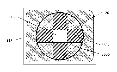
Other apertures can be designed to provide any desired exposure profiles. Some
examples are shown in Figure15B, Figure 15C and Figure 150. All the
collimators of Figure 15 have aperture design aimed at rotation of 360 degrees
for one EC.
The features of the apertures in the collimators of Figure 15 can be combined
with the features of the apertures in the collimators of Figure 13. Examples
for
such combinations are shown in Figure 16 showing 4 collimators with 4
different
aperture designs. In Figure 16A the left and right halves of the aperture are
not
symmetrical and one EC requires 360 degrees rotation. Figure 16B offers a
collimator with an aperture providing an exposure profile similar (but not
identical)
to that of Figure 150 but one EC consists of 90 degrees rotation only. Figure
16C
offers a collimator with an aperture providing an exposure profile similar
(but not
identical)to that of Figure 15D but one EC consists of 360/8=45 degrees
rotation
only. Figure 160 offers a collimator with an aperture providing an exposure
profile similar (but not identical) to that of Figure 15D also but one EC
consists of
180 degrees rotation only.
Following these examples it is appreciated the invention may be implemented in
many designs and it is not limited to a particular design provided hereinabove
as
an example.
Pixel correction:
As explained above, pixels with different DPP per the collimator design and
use
are normalized to provide a proper display-frame. Normalization scheme is made
in accordance to the x-ray exposure scheme (i.e., collimator shape, speed and
position). Such normalization can be done on the basis of theoretical
parameters.
For example, in reference to Figure 7 and Figure 5, with collimator 500
rotating
as a constant speed, the pixels of the annulus incorporating sectors 702 and
704
receive 1/10 the dose of circular area 700 (in this example the angular span
508
of sector 506 is 36 degrees). For simplicity of this example it is assumed
that one
38
CA 2893671 2018-11-30
frame is read from the sensor every time an EC is completed (i.e., collimator
500
completes a rotation of 360 degrees). It is also assumed that all sensor
pixels are
of the same response to the image intensifier output and that the image
intensifier has uniform response and the x-ray beam from the x-ray tube is
uniform. The only built-in (i.e. system level) source of differences between
the
pixels is from the collimator and the way it is operated. In this example the
normalization based on the system design would be a multiplication of pixels
by
one or 2 factors that will compensate for the difference in DPP.
In one normalization example the values from the pixels of the annulus
incorporating sectors 702 and 704 can be multiplied by 10. In another
normalization example the values from the pixels of circular area 700 can be
multiplied by 1/10. In yet another normalization example the values from the
pixels of the annulus incorporating sectors 702 and 704 can be multiplied by 5
and the values from the pixels of circular area 700 can be multiplied by 1/2.
It would be appreciated that description, explanations and examples of this
invention, multiplication and division are completely equivalent and
expressions
like "multiplying by 1/10" is completely equivalent to expressions like
"divide by
10" and whenever multiplication by a value is mentioned it means also the
division by reciprocal value alternative and vise-versa. The same holds for
multiplication and division symbols used in equations. For example A/B
represents also A=C where C=1/B.
The example above is relatively simple since the normalization scheme
incorporates 2 knows areas with two known DPP. The situation can become
relatively more complicated with different collimators or collimator motion
scheme.
In the following example a change is introduced to the rotation of collimator
500.
Instead of constant rotation speed a variable rotation speed is used as
presented
in the following table for one EC (in the case of collimator 500: 360
degrees):
39
CA 2893671 2018-11-30
Sector # EC range (degrees) Angular rotation status
1 0-150 Constant speed 1
2 150-180 Constant positive acceleration
3 180-330 Constant speed 2
4 330-360 Constant negative acceleration
This rotation pattern together with the convolution with the image pixels,
especially in the acceleration sectors, makes it more difficult to estimate
normalization the factors.
In the example of the collimators of Figure 15C and Figure 15D, many "pixel
rings" (pixels at a certain distance from the center) need a suitable
normalization
factor. Production tolerances of the system that are not included in the
theoretical
estimation of the normalization factors might result in errors that will show
up as
ring patterns in the image displayed on monitor 118.
The following calibration method provides calibration that removes the need
for
theoretical estimation of the factors and also compensates for production
tolerances.
In this example any collimator of the invention can be used and any rotation
pattern that is fixed per EC can be used.
The multiple frame x-ray imaging system is set to include all the fixed
element
relevant to the imaging process (x-ray tube, the desired x-ray operation mode
i.e.
voltage and current, possible x-ray filter, collimator, patient bed, image
intensifier,
camera) but none of the variable parts (the patient, the operator's hands and
tools).
40
CA 2893671 2018-11-30
According to this calibration method, the desired collimator is rotated in the
desired pattern. A set of raw frame is acquired (using any of the example
methods mentioned above). A raw frame is a frame resulting from an integer
number of one or more EC with all the pixels of are 712 (Figure 7), without
any
manipulation of the pixels. The number of raw frames acquired should be enough
to get a relatively good SIN on an average raw frame that is the average of
the
acquired raw frames. An average raw frame with S/N that is 10 times higher
than
that of the raw frame is typically sufficient and this can be achieved by
averaging
100 raw frames. It would be appreciated that more or less raw frames can be
used, depending on the desired quality of the normalized frame.
One average raw frame is created with x-ray off and another with x-ray on.
For this example we assume that the brightness value for each pixel for
display
purpose ranges from zero to 255. We also select to display a theoretical
noiseless frame in the range 5+250 (darkest noiseless pixel is displayed at
value
5 and the brightest exposed noiseless pixel is displayed at value 250. This
enables noise that brings the pixel values to the range 0+4 and 251+255
contribute its statistics appearance to the displayed-frame).
The correction for each pixel i of raw frames j, Pij (j is a frame number
index in
this example) is calculated using the values of the pixels of the average raw
frame made with x-ray radiation on, Al, and values of the pixels of the
average
raw frame made with x-ray radiation off, Bi, to produce the corrected pixel
Dij as
follows:
(Equation 1) Dij = (Pij ¨ Bi) = (245 / Al) + 5
In yet a somewhat more simple approach the correction might ignore noise
visual
aspects at the dark and bright level and simply correct to the display range
0+255
as follows:
(Equation 2) Dij = (Pij ¨ Bi) = (255 / Al)
41
CA 2893671 2018-11-30
It would be appreciated that the correction suggested above is linear and
works
best for systems with relatively linear response of the image intensifier and
the
camera.
For systems with non linear response, more complicated correction schemes
may be used such as bi-linear correction. In this example the range of the
values
of the pixels is divided roughly to 2 ranges. The current of the x-ray can be
reduced, for example to 1/2 its' normal operation mode so that the DPP is
reduced to 1/2. It is appreciated that the reduced current level depends on
the
nature of the non linearity and optimal bi-linear correction might require
other
than 1/2 of the x-ray current. It would also be appreciated that DPP can be
reduced also in other ways such aluminum plates placed right after the
collimator.
In this example, with 1/2 the x-ray current, another set of raw frames is
acquired.
It would be appreciated that the SIN of these raw frames is lower than that of
the
raw frames of the standard x-ray current for the specific application. This
can be
compensated by using more raw frames to generate the average raw frame for
1/2 the x-ray current, for example 200 raw frames. Let Mi represent the values
of
the pixels of the average raw frame made with 1/2 x-ray current radiation on.
The correction example of Equation 2 is implemented in this example as
follows:
For Pij with values less or equal 127
(Equation 3) Dij = (Pij ¨ Bi) = (127 / Mi)
For Pij with values higher than 127
(Equation 4) Dij = (Pij ¨ Bi) = (255 / Ai)
It would be appreciated that the x-ray current for Mi might be set to a
different
level (for example 1/4 of the standard current for the specific application)
and the
equations will assume the form:
For Pij with values less or equal 63
42
CA 2893671 2018-11-30
(Equation 5) Dij = (Pij ¨ Bi) = (63 / Mi )
For Pij with values higher than 63
(Equation 6) Dij -= (Pij ¨ Bi) = (255 I Ai )
It would also be appreciated that if the non-linearity of the pixels is
similar
between the different pixels within the operating range of the system (that is
differences in non linear response are relatively small) correction for non
linearity,
in most cases is not required. If the application does not require linear
response
and it is only desired to reduce pixels response non uniformity affects on the
displayed frame, then one may skip non-linearity correction.
All pixels corrections can be skipped if the noise pattern resulting from this
does
not disturb the application. The correction can be made at different
sophistication
levels (linear, bi-linear, tri-linear, polynomial interpolation and so on) or
not at all,
as suitable for the application.
Variable ROls and variable rotation speed profiles:
In the above examples different rotation profiles with different rotation
speeds
were described. In the following example rotation profiles of variable speed
will
be described in the context of ROI in the image. In the examples of the
collimators above, a central circular area (such as 600 of Figure 6 and 700 of
Figure 7) was presented as the ROI and therefore receiving more DPP than the
annulus of sectors 702 and 704 that receive lower DPP. This is the trivial
case
and typically the central area of the image is also the ROI, where the more
important part of the image is located. The higher DPP results in higher S/N
in
this area and therefore provides a better image quality in that area (such as
better distinguishable details). Normally, during, for example of a catheter
insertion procedure, the patient's bed is moved during the process to keep the
tip
of the catheter in the range of area 700. Yet, sometimes the area of highest
interest in the image moves out of area 700. For example, in reference to
Figure
17A, to the area denoted by numerical indicator 1700. This might be a result
of
43
CA 2893671 2018-11-30
many reasons such as (1) the catheter tip has moved to area 1700 and the
patient has not been moved to bring the catheter tip to area 700 (2) the
operator
is looking at area 1700 for any reason. This new ROI information can be fed as
input to the system in many ways including automatic follow-up of the catheter
tip
or follow-up of the area at which the operator looks using an eye tracker
device
(such as EyeLink 1000 available from SR Research Ltd., Kanata, Ontario,
Canada) to indicate the desired ROI location to be in conjunction with the
gazing
point of the user or by using a computer mouse to indicate the desired ROI
location.
With angular span of aperture sector 702 and at a constant rotation speed of
collimator 500, the DPP in the annulus outside area 700 is 1/10 of the DPP
inside
circular area 700 and SIN in the annulus outside area 700 is 1/10112 of that
of
area 700, resulting in a lower image quality. To overcome this and maintain
refreshment rate of the displayed frames of 10 fps with collimator 500 EC of
1/10
of a second as in the basic example of the invention, the rotation profile can
be
modified so that the collimator rotation speed in sector 1702 (Figure 17B)
that
contains area 700 is reduced to 1/10 of the uniform speed and the rotation
speed
at the rest of the EC is increased to maintain EC of 1/10 of a second.
This will be explained now in reference to Figure 17B, and the corresponding
flowchart in Figure 30 with example of actual numbers.
Let us assume that the angular span of sector 1702 that just contains area
1700
is 54 degrees (step 3000). The first edge of sector 1702 is 1702A and is
located
at angular position 63 degrees and the second edge of sector 1702 is 1702B and
is located at angular position 117 degrees. That is, sector 1700 is centered
on
angular position 90 degrees.
In step 31010, the reduced rotation speed of collimator 500 is calculated for
area
1702, that will result in area 1702 having similar S/N to that of area 702.
44
CA 2893671 2018-11-30
In this example, when edge 702A of sector 702 approaches angle 63 degrees
(the location of 1702A) the rotation speed of collimator 500 is reduced to 1
rps.
This rotation speed is maintained until edge 7026 of sector 702 reaches the
position of edge 1702B (117 degrees). From this point the rotation speed of
collimator 500 is increased again. In step 3020 the increased rotation speed
of
collimator 500 in area 704 is calculated, that will compensate for the change
of
speed in area 1702, to leave the total rps unchanged. For simplicity it will
be
assumed that acceleration and deceleration are extremely high and therefore
acceleration and deceleration times are definitely negligible for this
example. Per
the explanation above, collimator 500 rotation profile then includes 54+36=90
degrees (1/4 of the EC rotation) at a speed of 1 rps. To compensate for this
and
complete the EC at an average of 10 rps the rotation speed of collimator 500
at
the rest 3/4 of the EC rotation must be increased to Xrps, satisfying the
following
equation:
(Equation 7) 1rps451/4 + Xrps.3/4=1Orps
Therefore:
(Equation 8) Xrps = (lOrps - 1rpse1/4) 1(3/4) = 13 rps
That is, during the rest of the 270 degrees rotation of the EC, the rotation
speed
should be 13 rps.
With this rotation profile sector 1702 is exposed to the same DPP as area 700
and the SIN of area 1700 is also the same as area 700 as desired.
It would be appreciated that in the sector range outside sector 1702, for
which
the collimator rotation speed is increased to 13 rps, the DPP is reduced below
that of the DPP of constant rotation speed to 1/13 the DPP of area 700.
It would also be appreciated that area 1700 was presented here as an example
do demonstrate the design of rotation profile according to different ROI
geometries. Area 1700 might be different in shape and location and it might be
possible that more than one ROI is added to the basic ROI of circle 700. Such
CA 2893671 2018-11-30
variations are handled with profile variations of the same concept described
above.
It would also be appreciated that acceleration and deceleration mentioned
above
might take unreliable part of the EC and must be accounted for. Let us assume
in
the next example that acceleration and deceleration occupy 45 degrees of
rotation each and that they are uniform. In this case acceleration has to
start 45
degrees before edge 702A arrives at the position of edge 1702A and
deceleration starts when edge 702B arrives at the position of 1702B. All other
.. parameters of the system are the same. If X indicates the rotation speed
during
the 180 degrees of EC and Y is the average rotation speed during each of the
45
degrees acceleration deceleration sectors then the following equation needs to
be satisfied to maintain EC of 0.1s (or average rotation speed of 10 rps):
(Equation 9) 1rps01/4 + 2=Yrps.1/8 + Xrps.1/2 = 10 rps
Given constant acceleration and deceleration between 1rps and 10 rps,
Y= (1+10)/2=5.5 and the high rotation during 180 degrees is 16.75 rps.
It would be appreciated that this approach presented through the example above
is applicable also to other acceleration profiles, other collimators and other
operation schemes (such as different fps rates). It would also be appreciated
that
pixel correction methods described above are fully applicable also to variable
rotation speed profiles,
Different refreshment rates for different areas of the image:
It has been presented above (with the example of collimator 500 of Figure 5
and
operation mode of constant rotation speed of the collimator at 10rps and
display-
frame refreshment rate of 10 fps) that the DPP of circular area 700 of Figure
7 is
10 times higher than the DPP of the annular area constructed of sectors 702
and
704 (to be denoted "annulus" for short). Therefore the S/N in area 700 is also
101/2 better than the S/N in the annulus area. The refreshment rate of the
entire
image 120 (Figure 2) is the same: 10 fps. The temporal resolution of the
entire
46
CA 2893671 2018-11-30
frame is 0.1 second (s). In the previous example, each display-frame was
constructed from the data of one frame acquired from camera 116. Area 200 on
the display 118 is equivalent to area 700 on the sensor. Area 200 is exposed
to
times the DPP of area 202 and the SIN in area 200 is 101/2 better than the SIN
5 the annulus area 202. With each EC of collimator 500 the data is read
from
sensor 714, processed and displayed on monitor 118. The complete image 120
is refreshed then every 0.1s.
In the following example of the invention it is desired to improve the SIN of
10 annulus 202.
In a first example, while area 200 is refreshed every 0.1s with the data read
from
sensor 714, annulus 202 is refreshed only every Is. During this is, the data
received from sensor 714 for pixels of annulus 202 is used to generate an
annulus image that is the sum of the 10 previous frames. In a simplified form,
all
10 frames indexed j = 1 to 10 are stored. Then for each pixels i in the range
of
annulus 202 the sum of values is calculated: Pni = Epij. Pni are then
corrected
and displayed where n is index number for every set of 10 frames. Therefore
for
j = 1 to 10, the pixels of the sum frames is P1i. For frames j = 11 to 20, the
pixels
of the sum frames is P2i. For frames j = 21 to 30, the pixels of the sum
frames is
P3i and so on. With this example therefore we get a display of image 120 where
the S/N of annulus 202 is similar to that of area 200 although annulus 202
receives 1/10 of the DPP in every unit time of area 200. The compromise is
that
annulus 202 is refreshing every is comparing to every 0.1s of area 200 and the
temporal resolution of annulus 202 is is comparing to 0.1s of area 200.
In a second example, after the first 10 frames indexed j = 1 to 10 were
acquired
and stored and displayed as the sum of the pixels for annulus 202, refreshment
of annulus 202 is made in a different way. Instead of keeping the display of
annulus 202 for is until j = 11 to 20 are acquired, the displayed image is
refreshed after 0.1s as follows:
47
CA 2893671 2018-11-30
Frame j=11 is acquired and stored instead of frame 1. Therefore the previously
stored frames 1,2,3,4,5,6,7,8,9,10 the following frames are stored:
11,2,3,4,5,6,7,8,9,10. This set of frames is handled in the same way as the
pervious set and annulus 202 is refreshed. After additional 0.1s frame indexed
12
is acquired and is stored instead of the frame indexed 2:
11,12,3,4,5,6,7,8,9,10.
The set is now processed in the same way and annulus 202 display is refreshed.
This process repeat itself and as a result annulus area is refreshed every
0.1s,
same as area 200. The temporal resolution of annulus 202 is still is comparing
to area 200 with temporal resolution of 0.1s. The S/N in annulus 202 is
similar to
the S/N of area 200.
In a third example, an intermediate approach is presented. Following the first
example, instead of summing pixels of 10 frames and refreshing annulus 202
every is, summing can be done every 5 frames and refreshment od annulus 202
can be made every 0.5s. The S/N of annulus 202 is now 1/21/2 of the S/N of
Area
200 but still better than 1/101/2 of the basic example of collimator 500 and
the
temporal resolution is only 0.5s comparing to is of the first example of this
method.
It would be appreciated that also in the second example an intermediate
approach can be used where, instead of replacing each time one of 10 frames,
the replacement is of one frame in a set of 5 frames: 1,2,3,4,5 then 6,2,3,4,5
then
6,6,3,4,5 and so on. Here we gain again the refreshment of annulus 202 every
0.1s but with temporal resolution of 0.5s and S/N of annulus 202 is now i/21'2
of
the S/N of Area 200 but still better than 1/101/2 of the basic example of
collimator
500.
It will be appreciated that this method can be implemented also for
collimators
that are not rotating collimators such as the one of Figure 18. Figure 18A
provides a top view of the collimator and Figure 18B is cross section c-c of
Figure
18A. Collimator 1800 provides a similar function of x-ray reduction as other
48
CA 2893671 2018-11-30
collimators of the invention. It has an aperture 1802 that allows all the
radiation in
that area pass through, annulus 1806 that reduces the radiation passing
through
the area at amount depending on the material (typically aluminum) and the
thickness of the material and annulus 1804 with thickness changing as a
function
of the distance from the center, starting at thickness zero on the side of
aperture
1802 ending at the thickness of annulus 1806 on the side of annulus 1806.
Figure 18C provides a schematic DPP graph as a function of distance from the
center: r.
It is assumed that beyond annulus 1806 radiation is fully blocked. For the
purpose of the description of this example radiation that is scattered from
collimator 1800 is ignored. For this example it is also assumed that DPP
passing
through annulus 1806 is 1/10 the DPP passing through aperture 1802. Frame
rate is 10 fps and display-frame refreshment rate is 10/s. As described in the
above examples SIN of the image part associated with annulus 1806 is 1/101' of
the SIN associated with aperture 1802. To display an image where the SIN of
the
area associated with annulus 1806 is similar to the S/N in the area associated
with aperture 1802 any of the methods above can be used.
Figure 18D provides a representation of monitor 118 with the displayed frame
associated with collimator 1800. Circle 1822 is the area associated with
radiation
arriving through aperture 1802 of collimator 1800. Annulus 1824 is the area
associated with radiation arriving through annulus 1804 of collimator 1800.
Annulus 1826 is the area associated with radiation arriving through annulus
1806
of collimator 1800. It would be appreciated that while the example of annulus
1804 in Figure 18B is linear change of thickness, the example of change in
radiation of 1814 in Figure 18C is of a non-linear thickness change. That is,
many
different functions can be used to generate gradient in thickness 1804 to suit
the
desired gradual change in radiation between annulus 1800 and annulus 1806 of
Figure 18B.
49
CA 2893671 2018-11-30
In a first example, while area 1822 is refreshed every 0.1s with the data read
from sensor 714, annulus 1826 is refreshed only every Is. During this is, the
data received from sensor 714 for pixels of annulus 1826 is used to generate
an
annulus image that is the sum of the 10 previous frames. In a simplified form,
all
10 frames indexed j = 1 to 10 are stored. Then for each pixels i in the range
of
annulus 1826 the sum of values is calculated: Pni = ypij. Pni are then
corrected
and displayed where n is index number for every set of 10 frames. Therefore
for
j = 1 to 10, the pixels of the sum frames is P1i. For frames j = 11 to 20, the
pixels
of the sum frames is P2i. For frames j = 21 to 30, the pixels of the sum
frames is
.. P3i and so on. With this example therefore we get a display of image 120
where
the SIN of annulus 1826 is similar to that of area 1822 although annulus 1826
receives 1/10 of the DPP in every unit time of area 1822. The compromise is
that
annulus 1826 is refreshing every Is comparing to every 0.1s of area 1822 and
the temporal resolution of annulus 1826 is 1s comparing to 0.1s of area 1822.
For annulus 1824, we shall use here the example where the DPP decreases
linearly over the width of annulus 1820 from DPP of 1822 to 1/10 of this DPP,
the
DPP of annulus 1826.
In this example one may divide annulus 1824 to 8 annuluses of equal radius
step
so that the average DPP in the smallest annulus #1 is 9/10 of 1822, the
average
DPP in the next annulus #2 is 8/10 of 1822, annulus #3 is 7/10 and so on until
the last annulus #8 that has 2/10 DPP of 1822.
Whenever a value is mentioned in reference to the above segments (annuluses
#1 through #8) the value is the average value of that segment in consideration
of
the thickness variation of the collimator over that segment.
When the purpose is to provide on the entire displayed image 120 the same S/N
and keep temporal resolution of up to Is, it can be done in a simple way for
annulus #5 (1/2 DPP than in area 1822) and annulus #8 (1/5 DPP of area 1822)
CA 2893671 2018-11-30
since the ratio of DPP in area 1822 and the DPP in annulus #5 is an integer.
The
same is the case for annulus #2.
In the case of annulus #5 adding 2 temporally successive frames as described
in
any of the above methods (with adequate pixel correction as described above)
provides S/N similar to area 1822. Temporal resolution in this example is
0.2s.
In the case of annulus #8 adding 5 temporally successive frames as described
in
any of the above methods (with adequate pixel correction as described above)
provides S/N similar to area 1822. Temporal resolution in this example is
0.5s.
For other annuluses (#1, #3, #4, #6, #7 and #8) the ratio of DPP in area 1822
and the DPP in any of these annuluses is not an integer. Therefore adding
pixels
of an integer number of frames (up to 10 considering the desired limit of not
more
than Is temporal resolution) will exceed the desired S/N or be less than the
desired S/N.
To achieve the desired S/N under the requirements of this example, the
following
method (which is described by flowchart in Figure 31) can be applied:
1. For each annulus #m add the minimum number of pixels of temporally
successive frames that provide S/N equal or higher to the S/N of area
1822 (steps 3100 ¨ 3120).
2. Execute pixel correction (offset, normalization and so on as described
above) (step 3130).
3. Add noise to each pixel in annulus #m compensate for the cases of S/N
higher than in area 1822 (steps 3140-3150).
The above steps will be discussed in more details in reference to annulus #1.
The DPP in annulus #1 is 9/10 the DPP of area 1822. The S/N in annulus #1 is
.. (9/10)1/2 of the S/N in area 1822. Therefore, according to step 1 above we
need
51
CA 2893671 2018-11-30
to add pixels of 2 temporally successive frames in the area of annulus #1 to
make the S/N of the pixels in annulus #1 equal or higher than that of area
1822.
By adding the pixels of 2 temporally successive frames in the area of annulus
#1
the effective DPP in the resultant frame in annulus 1 is 18/10 of the DPP in
area
1822. The S/N in annulus #1 is now (18/10)1/2 of the S/N in area 1822. To
compensate for the too high S/N (and therefore result in possible visual
artifacts
in image 120, a Gaussian noise is added to each pixel to satisfy the equation:
(Equation 10) (N1822)2= (N#1)2 + (Nadd)2
Where N1822 is the noise associated with a specific pixel in area 1822 for a
specific object transmission, N#1 is the noise associated with the pixel that
is the
sum of 2 temporally successive pixels in annulus #1 (sum-pixel), having the
same object transmission and after the sum-pixel has gone through pixel
correction process (including, in the simplest correction form, dividing the
value
of the summed pixels by 1.8 to bring the affective DPP from 18/10 to 10/10 ¨
the
same as in area 1822) and Nadd is the noise to be added to the sum-pixel to
bring
its S/N to the same level as the equivalent pixel in area 1822.
In the example above, since the number of x-ray photons in the sum pixel of
annulus #1 is 1.8 of the equivalent pixel (same object transmission) of area
1822,
the noise of the sum-pixel is (1.8)1/2 of the equivalent pixel in area 1822
and the
S/N is also (1.8)1/2 of the equivalent pixel in area 1822.
To calculate the amount of Nadd we use equation 10 in the form:
(Equation 11) Nadd = ((N1822)2 - (Nwi)2)1/2
With the pixel correction division by 1.8.
Using numbers:
Nada = (12¨ ((1 .81/2) / 1.8)2)1/2
Nadd = 0.667
52
CA 2893671 2018-11-30
Therefore, by adding this Poisson noise to the sum pixel we provide to that
pixel
a noise that is similar to the equivalent pixel in area 1822.
It is appreciated that all examples are calculated on a relative basis and
therefore
the pixel of area 1822 is 1.
It would be appreciated that the noise values in equation 10 are dependent on
the pixel value and are typically the square rout of the pixel average level.
The same correction method is applicable to all the segments of annulus 1824
with suitable adjustments.
It would be appreciated that adding pixels of successive frames can be done by
adding new frames each time before display-frame refreshment or using the
FIFO method as described above.
It would be appreciated that dividing annulus 1824 to 8 segments (Annulus #1
through annulus #8) is provided as an example only. The higher the number of
segments, the more uniform the S/N is over annulus 1824. Yet, the visibility
of
the non uniformity of the S/N adjustment is obscured by the S/N of the image
therefore, above a certain number of segments the visual contribution of more
segments is low and might be undistinguishable to the operator. Therefore one
may limit the number of annulus segments in accordance to the S/N statistics
of
the image in the specific procedure.
.. The same methods for handling the non-uniform DPP regions such as annulus
1824 of the collimator example 1800 can be used also for collimators of the
present invention such as those of Figure 15C, Figure 15D and all the
collimators
of Figure 16 that also produce non-uniform DPP regions. These methods can be
used with any collimator that generates different exposure regions, regardless
of
the method used by the collimator, whether the different exposure regions are
generated by the shape of the collimator, by a motion of the collimator or by
53
CA 2893671 2018-11-30
combining shape and motion. In all cases of motion of the collimator cycles of
the
same motion pattern simplify the image enhancement as described above but it
is not a requirement to allow the image enhancement described above.
In the above example, in reference to the image area 1826 (Figure 18D)
corresponding with annulus 1806 (Figure 18A), the discussion referred to basic
processing of image area 1826: since the radiation there is 1/10 of the
radiation
in area 1822, one can sum last 10 frames in area 1826 to generate a processed
1826 area with SIN similar to that of area 1822.
In another approach, one may compromise SIN goal in area 1826 for adding less
frames. For example, one may prefer summing only 5 frames and get S/N that is
0.71 of the SIN of area 1822 but, by doing so, improve temporal resolution of
area 1826 by a factor of 2 compared to the case of summing 10 frames.
To compensate for the resulting 1/2 brightness in this example, each pixel
value
in area 1826 can be multiplied by 2. More generally, if one needs to sum M
frames to get the brightness that is in conjunction with the brightness of
area
1822, and instead m frames are summed (m can be any positive number), the
pixel values of the pixels in area 1826 should be multiplied by M/m.
It would also be appreciated that the number of summed frames does not have to
be an integer. For example, 4.5 frames can be summed. In this example FRMn is
the last frame, FRMn-1 is the previous frame and so on. Summing last 4.5
frames can assume the form (for each pixel):
SUM= (FRMn)+(FRMn-1)+(FRMn-2)+(FRMn-3)+0.5X(FRMn-4)
Brightness adjustment then uses the factor 10/4.5.
In some cases, due to the spectral change in radiation that goes through
annulus
1806 (and also 1804), the x-ray in that area experiences a lower absorption
coefficient when passing through the patient. Therefore, although when no
54
CA 2893671 2018-11-30
patient or other absorbing matter is present the radiation for area 1826 is
1/10
that of the radiation for area 1822, when an absorbing object is present the
effective radiation for area 1826 relative to that for area 1822 is higher
than 1/10.
It might be, for example, 1/8. In such a case, adding 8 last frames satisfies
both
the S/N and brightness criteria (being similar to that of area 1822). This can
be
used to sum less frames, especially in dark areas (high absorption
coefficient).
In yet another example of the invention when the ROI shifts to area 1700 as
presented in Figure 17A, instead of adjusting the rotation profile of
collimator 500
as explained in reference to Figure 17B, the whole collimator can be displaced
linearly, in direction parallel to the plane of collimator 500, so that the x-
ray
radiation passing through circular aperture 504 of Figure 5 is now centered
about
area 1700 as shown in Figure 19A on camera sensor 710.
It is assumed that the only radiation that can arrive at the collimator input
surface
112 is radiation that passes through the aperture of collimator 500 (circular
hole
505 and sector hole 506). Therefore area 1902 in the sensor is shadowed out in
Figure 19A (no radiation arrives at the corresponding area of image
intensifier
input 112) and only the area including 700, 702 and 704 limited by boundary
712
is exposed. The exposed area is then the overlap between two circles with
centers shifted one relative to the other and indicated in Figure 19A by the
numerical indicator 1900.
This desired function of the invention is provided here within area 1900 by
circular hole 504 that enables higher DPP in area 700 and sector hole 506
associated with the rest of the image area enabling only 1/10 of the DPP of
hole
504.
Figure 19B illustrates the appearance version of Figure 2 according to the
.. example of Figure 19A.
CA 2893671 2018-11-30
Collimator 500 can be moved in X-Y plane (see coordinate system 126 of Figure
1A) using any common X-Y mechanical system. For example, annulus shaped
static part 1016 of Figure 10C is connected to an X-Y system instead of being
connected to the x-ray tube structure and the X-Y system is connected to the
structure of the X-Y tube, thus enabling the collimator of Figure 10C, in this
example, to move in X-Y plane as desired for the example of Figure 19A.
It would be appreciated that the above methods such as pixel correction, SIN
adjustments, adding pixels of different frames are fully applicable to the
example
of Figure 19A with the adjustment of to the displacement of the collimator.
The X-
Y shift method is applicable to any of the collimators of this invention.
It would be appreciated that also displacement along a line (X axis for
example)
instead of X-Y can be applied in the same way with the limitation of ROI areas
that can be handled this way over image 120 area.
X-Y mechanical systems can assume many designs, including such as Motorized
XY Table ZXWO5OHAO2 available from Shanghai ZhengXin Ltd, Shanghai,
China. The custom design of X-Y mechanical systems is common in the art and
is often made to optimally suit the needs of the application. One such
provider of
custom designed X-Y mechanical systems is LinTech, Monrovia, California, USA.
It would be appreciated that the diameter of collimator 500 can be increased
so
that the length of sector 702 is increased to r3 as shown in Figure 20B.
Figure
20A is the collimator of Figure 5 provided here as Figure 20A for easy
comparison with the collimator of Figure 20B. Angle 508 is the same (36
degrees
in this example), the diameter of circular hole 504 is the same (r1). R3 is
large
enough to incorporate the complete field of view of image intensifier input
112
also when the collimator is displaced laterally as explained in reference to
Figure
.. 19. With this design, the complete image area 120 of Figure 19B remains
active
56
CA 2893671 2018-11-30
without any shadowed area such as 1902 in the example of Figure 19. This
collimator enlargement can be implemented in any collimator of the invention.
For the example of Figure 19, where the maximum displacement desired is up to
the point that the edge circular hole 700 is just in one point contact
anywhere on
the edge of image 712 edge (such one example point is point 1904 in Figure
b19A) the required radius r3 of the sector hole can be calculated as follows,
in
reference to Figure 20B:
(Equation 12) r3 = A ¨ r1
Where A is the diameter of the image intensifier input 112 B (see Figure 3)
scaled to its' projection in the collimator plane. That is:
(Equation 13) A= B.(D1/D2)
In the process of moving the collimator in X-Y plane, pixels that have been
exposed to full DPP (through area 504) may change status to be exposed at 1/10
DPP since area 504 has moved and such pixels are not included in that area
anymore. It would be appreciated that Is a pixel has changes status from being
included in area 504 and full DPP to be outside area 504 and 1/10 DPP,
considering the operation mode of this example, 10 frames of 1/10 DPP have
been already acquired and the processing of this pixel for display is made in
any
of the methods described above that use last 10 frames to provide S/N same as
within area 504 (or 5 frames after 0.5s in another example). During the is
transition another handling is required to keep the S/N of this pixel the same
as it
was when it was included in area 504.
Reference is made to Figure 32. In step 3200, pixels from the current frame
are
added to the pixel sum, and the next frame is considered (step 3210). The
frames summed thus far in the transition period are combined in a weighted sum
with the full DPP data (step 3220), where the full DPP data is weighted in
order
to compensate for the lower DPP of the new frames and retain a consistent S/N.
For instance, one frame into the transition, the display will be a weighed sum
of
57
CA 2893671 2018-11-30
90% full DPP and the one new frame. After two frames, 80% full DPP and the
two new frames, and so on. The weight of the full DPP attenuates its effective
dose to represent the DPP necessary to keep the S/N of the pixels the same as
it
was when they were included in area 504.
In step 3230, normalization if performed, and then the updated image is
displayed (step 3240). The process continues for a full EC, where the new
frames progressively receive more weight compared to the old full DPP data.
When 10 frames have passed, the transition period is over and methods such as
the one described in Figure 28C can begin to operate (step 3260).
An example is provided below for further clarification: In this example, with
refreshment rate of 0.1s and temporal resolution that varies from 0.1s to is
the
following procedure is implemented, where N is the index of the last full DPP
frame for that pixel:
1. At time 0 display for the pixel 100% the last full DPP data of frame N.
Temporal resolution is 0.1s.
2. At time 0.1s display for the pixel a weighted sum of 90% the last full DPP
data
of frame N and 100% of the new DPP data of frame N+1.
3. At time 0.2s display for the pixel a weighted sum of 80% of the last full
DPP
data of frame N, 100% of the DPP data of frame N+1 and 100% of the DPP
data of frame N+2.
7. ....
10.At time 0.9s display for the pixel a weighted sum of 10% the last full DPP
data
of frame N and 100% of the new DPP data of each of frames N+1,
N+2,.. .,N+9.
58
CA 2893671 2018-11-30
11 .At time 1.0s display for the pixel a weighted sum of 0% the last full DPP
data
of frame N and 100% of the new DPP data of each of frames N+1,
N+2 .N+9, N+10. Temporal resolution has now changed to Is.
12.Continue with methods described above for image improvement for 1/10 DPP
regions. Temporal resolution is is.
It would be appreciated that in the case of the method of refreshing the
pixels of
1/10 DPP in a rate of only 1 fps the last full DPP data is presented for Is
after the
change of the pixel to 1/10 DPP exposure and afterwards the average of the
last
10 frames of 1/10 DPP will be used to refresh the pixel.
In the case that a pixel changes status in the opposite direction, that is
changing
from 1/10 DPP area to full DPP area, this transition is instant and in the
first 0.1s
after the status change the displayed image is refreshed with the first 0.1s
frame
of the full DPP.
It would be appreciated as explained in reference to Figure 1A, that the above
methods are applicable also for relatively high frequency pulse x-ray. The
term
"relatively high frequency" is relative to the collimator design and operation
mode. In the example of collimator 500 of Figure 5, that has a sector angular
span of 36 degrees and rotates at 10 rps, the pulse frequency should be at
least
at a frequency of 100/s so that there is at least one x-ray pulse per each 36
degrees area of a frame. To simplify pixel correction scheme, it is also
desired
that the x-ray pulse frequency would be a positive integer multiplication of
minimum frequency. In this example: 200/s, 300/s, 400/s and so on. In this
example 1,000/s (10 times the minimum frequency can be considered relatively
high frequency.
It is appreciated that no collimator is totally opaque to x-ray and
collimators are
constructed to block most of the x-ray in the opaque regions. With HVL (half
value layer) of 0.25mm (similar to that of lead), 3mm thick collimator allows
0.50
59
CA 2893671 2018-11-30
0.25) = 1/4096 of the incident x-ray radiation to pass through (without
scatter). The
term "essentially opaque" will be used to describe these practical
collimators.
Most of the collimators described hereinabove are constructed of essentially
opaque region such as 518 of Figure 5 and apertures or holes as 504 and 506 of
Figure 5. Collimators such as the example of Figure 18 are different since, in
addition to the essentially opaque region 1806 and the aperture 1802 they
include semi-opaque regions such as 1804 of Figure 18A.
Collimators according to this invention can be mounted on an x-ray system as
__ stand-alone or together with another collimator, for example, such that is
designed to limit the x-ray to a part of input area 112 of the image
intensifier.
Collimators of the invention and other collimators may be placed in any order
along the x-rat path. The exposed part of area 112 is the remaining of the
superposition of the area all the collimators in the path of the x-ray block.
In the
__ design of such successive arrangement, the distances of each of the
collimators
from the x-ray source and distance to area 112 needs to be considered with the
geometry of the collimators, as described above, to get the desired
functionality.
Image optimization using dynamic ROI and eye tracker
In another example, any of the above examples of collimators and examples of
image processing (and also examples that are not described hereinabove) can
be used with an eye tracker to further enhance the image perceived by the
user.
In a typical multiple frame x-ray imaging system an area is defined, typically
centered about the center of the image, to determine what might generally be
called the brightness of the image. Sometimes contrast of the image is also
determined based on this area. Typically the area is smaller than the entire
image but it can also be an area of a size similar to the entire image.
Based on the image content in this area, various parameters related to the
image
quality might be determined to optimize the image for the user, such as:
CA 2893671 2018-11-30
1. x-ray tube current (whether in continuous or pulse modes)
2. x-ray tube Peak Kilo Voltage (PKV)
3. x-ray pulse length
4. AGC (Automatic Gain Control), whether analog or digital
5. Tone correction or tone-adjustment of the image implemented in various
functions such and brightness, contrast, gamma, offset, gain, n-degree
linear functions, non linear functions etc.
One example of optimizing the image according to the image content in this
area
is to identify the 10% brightest pixels in this area, calculate the average
value of
these pixels and adjust the gain (multiply each pixel value by a constant
factor)
so that the average value is set to level 240 in an 8 bit display system that
provides display levels 0 through 255.
The typical result of such parameters changes using the image data of the
defined area is that the image in that area is optimized to the content of
said
image for visual perception of the user while image parts outside this area
might
not be optimized for visual perception of the user.
For example, a lung may be present in the optimization area. Since the lung is
relatively transparent to x-ray radiation, the optimization operates to reduce
radiation to make the lung appear at a desired brightness. As a result, the
spine
that is nearby, but outside the optimization area, will appear dark and
visibility of
details might be lost. To overcome this with the present art, the patient is
moved
until the spine is in the optimization area and optimization is made for the
spine,
brightening it up. But now, the lung is too bright and lung details in the
image are
degraded. This conflict can be resolved by using x-ray manipulating
collimators
such as those described above with the eye tracker.
According to the present invention, the X Ray tube input parameters may be
controlled automatically or via user guided settings in order to
enhance/adjust
intensity (and obtain adequate image quality) within the ROI as well as the
61
CA 2893671 2018-11-30
periphery and guarantee that certain features (such as a stent, tool or
anatomy)
are apparent and clearly visible.
In the present example, the ROI is not static but instead it follows the
coordinates
of the eye gazing of the user. The eye tracker provides a stream of (x,y) of
the
gazing point of the user on the screen. The ROI is moved to these coordinates,
with a complementary adjustment of the collimator and the optimization is made
for the image included in the ROI ¨ where the user is gazing at.
As a result, the image is optimized in the area where the user is looking and
where he needs the best image at any time without a need for any manual
adjustments or compensations for the automatic image optimization function.
It would be appreciated that this function can be used throughout the
procedure
or only during desired intervals of the procedure.
The image may be optimized per the ROI content using any of the above
mentioned parameters or any other parameter that modifies the displayed value
of a pixel in the image.
It would also be appreciated that the ROI does not need to be centered at the
gazing point. The desired optimization can be made also when the ROI is
selected so that it contains the gazing point.
It would be appreciated that the above optimization method can be applied also
without using any of the above examples of collimators and examples of image
processing. This method can be applied to a multiple frame x-ray imaging
system
that employs generally uniform DPP over the field of view of image intensifier
input 112. An eye tracker is added to such a multiple frame x-ray imaging
system
to detect the gazing point of the operator in the image area. The above
.. optimization is made then for an image area that contains this gazing point
as
described above.
62
CA 2893671 2018-11-30
Background imaqe processing using tone-correction function
One of the effects of using a collimator of the type described in reference to
Figure 18A through Figure 18D is the change of the spectrum of the x-ray
radiation in the background (annulus 1806) Vs the ROI (Annulus 1802). The
result of reducing x-ray DPP through the background filter (annulus 1806) is a
change of the x-ray spectrum in that area of the image comparing to the ROI
area of the image (ROI in short). This in turn results in different absorption
characteristics of the x-ray in human tissue (or any other material) in the
background area Vs the ROI. In the example of the collimator associated with
Figure 18A through Figure 18D and considering also the example that the
background area photon count per pixel is 10% of the photon count per pixel in
the ROI in no presence of patient or phantom (110 of Figure 1A), one might
suggest that by multiplying each background pixel value by 10 (or by summing
last 10 background images as described above), the background image will
become similar to the image in the ROI. This is not the typical case.
Typically, a
more complex tone reproduction function is required to make the background
image look more similar to the ROI image. This is explained in more details in
reference to Figure 21A through Figure 21C.
It would be appreciated that the selection of 10% hereinabove is arbitrary and
made only as an example. Other values between 1% and 90% can be selected
as well as any value higher than zero and lower than 100%. The adjustment of
the description for values other than 10% is obvious for those skilled in the
art.
A typical tool used in the x-ray field for image research, measurements,
calibrations and evaluations is the 10 step wedge as shown in Figure 21A. It
can
be constructed of many materials. By placing such a step wedge in the x-ray
path
instead of patient 110 of Figure 1A, a stripes-image is acquired, the pixels
of
each rectangular stripe are of a relatively similar value comparing to the
63
CA 2893671 2018-11-30
difference between pixels of neighboring steps (assuming relatively high SIN).
Average value in each stripe can be measured to produce the values of the 11
dotted bars 2104 in Figure 21B. The horizontal axis represents the relative
step
thickness, number zero represents no absorption (a strip of air only), number
1
represents the thinnest step of step wedge 2100 and number 10 represents the
thickest step of step wedge 2100, being 10 times thicker than the thinnest
step,
in this example.
The vertical axis represents a pixel value. In this example a 12 bit system
was
selected providing a dynamic range of 0+4095. A 12 bit system was selected for
this example since it is a popular system in this field for digital image
processing
but it would be appreciated that that any system can be used to realize the
invention, that the adoption of the invention to other system is simple for a
person
skilled in the art and the scope of the invention is not limited by this
example.
Also, in this example, the average pixel level in air was set to 4000,
allowing 95
additional levels for pixel noise and avoid high noise digital cutoff at 4095.
This
selection is made as an example and it is appreciated that noise depends in
such
systems on the x-ray DPP and the value for air transmission should be made
according to the preferred x-ray characteristics.
In this example, the filtering of x-ray intensity in the background, that
results in
change of spectral distribution of the x-ray radiation in the background, will
change characteristics of absorption coefficient through the same step wedge
2100. The resultant pixel values for the background radiation for each step
are
shown as 11 black bars 2106 in Figure 21B.
When implementing a first process of the background by adding last 10
background frames as described above (or multiplying each background pixel by
10), the initially-processed background pixel value in step zero becomes
similar
to ROI pixel value in step zero as shown by the leftmost girded bar in the 11
64
CA 2893671 2018-11-30
girded bars 2108, representing the average value of the steps in the
background,
after adding last 10 frames.
By examining bars 2108 Vs bars 2104 it becomes evident that, except for step
zero, all 10 remaining 2108 bars are of higher values than the 10 remaining
bars
2104. This results from the different absorption in the background due to
spectral
change made by annulus 1806 of the filter of Figure 18A. For example, the
average pixel value of step 5 in the ROI is 1419 but in the initially-
processed
background it is 2005. This results in apparent difference between the
initially-
processed background image and the ROI image.
To resolve this, an additional processing step is required for the background
image area (background in short). Such a correction function, in reference to
the
ROI area and the background area of the steps of Figure 21B is shown as
function 2112 of Figure 21C and it will be called here tone-correction
function.
The process of changing an image using the tone-correction function will be
called here tone-correction.
Tone-correction function 2112 is created by calculating the tone-correction
factors for each of the 11 strips to bring the average value of the
backgrounds
strip to the same average pixel value of the strip in the ROI area. Each such
factor is the ratio of the average step pixel value in the ROI to the average
step
pixel value in the background. Factors for pixel values between these
calculated
values can be obtained using interpolation of any kind such as a cubical
interpolation or fitting of any function to the 11 calculated points such as
exponential or n-dimensional linear function. It is evident, in this example,
that
the lower the pixel value is, in the background area, the lower is the
correction
factor. For example, for initially-processed background pixel value 762 the
correction factor is 0.44 (2114 in Figure 21C). While for initially-processed
background pixel value 2524 the correction factor is 0.79 (2116 in Figure
21C).
CA 2893671 2018-11-30
Tone-correction in this example refers to the multiplication of each pixel in
the
initially-processed background by the associated factor per the example of
Figure
21C.
The tone-correction function of Figure 21C is used to further process the
initially-
processed background by multiplying each of the initially-processed background
pixels by the associated factor (Background pixel correction factor) provided
by
tone-reproduction function 2112.
It would be appreciated that although, in this example, background was
processed to become similar to the ROI but it is also possible to use the same
approach to process the ROI to become similar to the background. It is also
possible to execute the initial-processing on the background and execute the
tone-reproduction on the ROI relative to the background. One only needs to
exchange the words background and ROI in the example above to get a
description of such a tone-correction.
It is also appreciated that initial-processing that results in similar step
values for
ROI and background is not a requirement for tone-correction. The tone
correction
can be executed without the above initial-processing or with initial
processing
that, for example, is designed to bring the background step zero to be half
the
value of the ROI step zero. This can be done, for example, by adding 5 last
images instead of 10 last images in the present 10% background radiation. The
tone-correction process is the same, only the tone-correction function
(calculated
in the same way) is different.
Tone-correction function calculation using step wedge
In the following example a method is presented in more details, to generate a
tone-correction function for background image so to make it appear similar to
that
of the ROI. In this method reference is made to Figure 33A.
66
CA 2893671 2018-11-30
The first phase of this method is the data collection.
To collect the data variable absorption phantom is used to provide for
different
absorption levels through the image area. Such a phantom may consist of a step
wedge (such as the one of Figure 21A), a linear wedge phantom, a variable
thickness phantom of continuous slope function, a random thickness phantom or
any other variable absorption phantom that will provide enough measurement
points over the dynamic range of the image (0+4095 in a 12 bit system),
reasonably spread throughout the dynamic range to provide the desired
accuracy. It would be appreciated that the more steps that are more evenly
spread through the dynamic range ¨ the more accurate the tone-correction
function will be. A step wedge of 10 steps would be a reasonable choice for
reasonable accuracy.
The variable absorption phantom (VAP) preferred material would be a material
that behaves similar to live tissue. It is common to assume that water is a
reasonable representation of a live soft tissue. There are materials that are
considered water-equivalent that are used to produce such phantoms such as
Plastic Water available from Supertech, Elkhart, Indiana, USA. By using such
materials the data collection better resembles the response to live soft
tissue of
the filtered background radiation spectrum and ROI radiation spectrum.
Materials
that are bone equivalent can also be used in such a variable absorption
phantom
but anyone skilled in the art would understand that it is merely an extension
of
the soft tissue discussion and therefore it will not be discussed in more
details
here.
The variable absorption phantom (VAP) is placed in the system of Figure 1A
instead of patient 110.
67
CA 2893671 2018-11-30
An image, or a set of images are acquired for a given PKV1. The reason for PKV
being a parameter is the PKV dependent spectrum of the x-ray and thus, each
tone-correction curve is calculated for a given PKV. The acquired images are
designed so that, in the example of step wedge, each step is acquired with
each
of the x-ray spectrums of the ROI and the background. That is, either a part
of
the step is in the ROI and another part is in the background or, in one image
the
step is in the ROI and in another image the step is in the background.
Now, in this example, we choose to modify the values of the background pixels
and to use the ROI as reference and adjust the background to appear similar to
the ROI. It would be appreciated that the value of the pixels of the ROI can
be
adjusted to bring the ROI to look like the background (or other alternatives
can
be used as discussed above) but since the technique is completely analog to
the
present example it will not be discussed here in more details.
To do so, for each step i (including step zero of air) the average of 2 pixel
groups
are calculated:
1. (step 3300) pixels of step i that are in the ROI: AVGri
2. (step 3305) pixels of step i that are in the background: AVGbi
These two numbers are used (step 3310) now to calculate the tone-correction
function value for background pixel having the level AVGbi: F(AVGbi):
F(AVGbi) = AVGri / AVGbi
In the example of 10 steps step wedge + one step of air, a set of 11 tone-
correction function values is provided:
{F(AVGb0), F(AVGb1), F(AVGb2),..., F(AVGb10))
In the example of 12 bit display system, 4096 correction values are desired so
that each possible value of a pixel in the background has a correction tone-
correction function value. Such values beyond the 11 values calculated above
can be estimated using any interpolation and extrapolation approaches (step
68
CA 2893671 2018-11-30
3320) such as linear, 2nd degree or any n-degree linear function fit or
exponential
function fit etc. The concept is the same, the difference is in the accuracy
of the
calculated tone-correction function, evaluated typically by how similar the
background becomes to the ROI after the correction. This can be demonstrated
using the following example.
An example table is provided for a step wedge used to measure the function
values for each of the 10 steps plus the air step:
Step AVGri AVGbi F(AVGbi)
0 4000.00 4000.00 1.00
1 3733.02 3819.97 .. 0.98
2 3251.32 3483.85 0.93
3 2642.77 3034.31 0.87
4 2004.75 2523.83 0.79
5 1419.25 2004.75 0.71
6 937.69 1520.76 .. 0.62
7 578.18 1101.69 0.52
8 332.71 762.18 0.44
9 178.67 503.57 0.35
89.55 317.73 0.28
10 In this example, step zero is an area without absorption, an area
outside of the
VAP. In this example, the background has gone also through the initial
processing (such as adding last 10 frames to compensate for 10% background
radiation as described in details above). For this reason AVGrO = AVGb0. In
this
example also the exposure has been set so that AVGrO = 4000. For a given PKV
this is done by determining, for example, the mA (milliampere) in a continuous
multiple frame x-ray imaging system or determining the charge per pulse in a
pulsed x-ray system (milliampere-second: mAs). For the purpose of the
following
discussion we shall refer to mA-0 as indicating the x-ray current setup to get
AVGrO = 4000.
Therefore, to get the correction factors for 0+4095 an interpolation is needed
for
the range 319+3999 and extrapolation is needed for the ranges 0+317 and
69
CA 2893671 2018-11-30
4001+40095. This can be done using one of the many curve fitting methods
provided, for example, by MatLab, available from MathWorks, Inc., Natick,
Massachusetts, USA. The specific fitting method typically depends on the data.
It would be appreciated that not all steps must be used to calculate the tone-
correction function but, typically, using more steps supports a better tone-
correction function.
It would be appreciated that for the purpose of curve fitting, such a curve is
always expected to pass also through the point (AVGb, F(AVGb)) = (0,0). That
is,
when the absorber thickness is so high that the radiation is fully blocked by
this
thickness, the tone-correction value at this point is zero.
In accordance with the above example it can be illustrated with 2 additional
lines
in the table, presenting relative thickness of 200 and infinity:
_ Step AVGri AVGbi F(AVGbi)
200 0.00 0.03 0.0068
Do 0.00 0.00 0.00
This additional point (0,0) can therefore be additionally used, with any set
of
measurements, for a better curve fitting.
It would also be appreciated that more than just 2 image areas such as ROI
(1822 in Figure 180 corresponding to filter section 1802 in Figure 18A and
Figure
18B) ) and background (1826 in Figure 18D corresponding to filter section 1806
in Figure 18A and Figure 18B) are relevant to the tone-correction described
above. Other image areas such as transition area 1824 in Figure 18D
corresponding to filter section 1804 in Figure 18A and Figure 18B are
relevant. In
the example of transition area 1824 the spectrum of the x-ray changes
gradually
as a function of distance from the ROI center due to the variable change in
the
filter thickness over annulus 1804. It would be appreciated that the tone-
correction curve designed for background 1826 will not be optimal for
transition
area 1824.
CA 2893671 2018-11-30
It is desired therefore to divide transition area 1824 into a number of
transition
sub-areas, each transition sub-area has a relatively uniform x-ray spectrum
after
filtering. For each such transition sub-area a tone correction function is
calculated
(for each PKV) and is used to tone-correct the associated transition sub-area.
In another approach, the tone-correction function for a specific sub-area can
be
estimated from the tone-correction function of the background, taking into
account the filter thickness in the specific transition sub-area. For example,
for a
transition sub-area thickness near that of the background, the tone correction
function will be close to the tone-correction function of the background. One
example for such an estimation of tone-correction values is provided in the
following table
Near Near
Step background background
ROI
0 1.00 1.00 1.00
1 0.98 0.98 1.00
2 0.93 0.94 1.00
3 0.87 0.89 0.99
4 0.79 0.82 0.98
5 0.71 0.75 0.98
6 0.62 0.66 0.97
7 0.52 0.58 0.96
8 0.44 0.49 0.94
9 0.35 0.41 0.93
10 0.28 0.34 0.92
The values for "Near background" and "Near RD I" are estimated from the
background values using exponential evaluation in the form:
Estimated_value = Background_valueE
Where E=0.85 for the "Near background" values estimation and E=0.07 for the
"Near ROI" values estimation.
71
CA 2893671 2018-11-30
Many other estimations can be used. The exponential estimation reasonably
supports the exponential absorption characteristics of x-ray in matter.
The above method is executed for a range of PKV values to generate a tone-
correction function for each such PKV value. For example, in the range of
50PKV
to 150PKV, 5 tone-correction functions can be generated for 50, 75, 100, 125
and 150PKV.
In case, for example, that 90PKV is used with a patient, the tone-correction
function can be interpolated from the tone-correction functions calculated for
75PKV and 100PKV using linear interpolation or any other interpolation. The
interpolated tone-correction function can now be used for tone correction of
the
background generated with 90PKV radiation.
A common situation that might be encountered after executing the above tone-
correction function calculation is that the actual image in use does not
contain air
sections and also maybe does not contain objects equivalent to steps 1, 2, 3
and
4. It is possible, for example, that the most "x-ray transparent" part in the
examined object (patient 110 in Figure 1A) reaches only level 2000 out or the
0+4095 dynamic range. In such a case the x-ray current might be doubled to
increase the DPP so that this area is brightened-up and arrives to level 4000.
In such a case, the tone-correction value originally designed to 4000 is not
suitable anymore since the current 4000 is generated after absorption
equivalent
to the 2000 level of the tone-correction function.
To handle this situation, if the x-ray mA is doubled so that current mA is
2x(mA-
0), one can modify the x-axis units of the tone-correction function of Figure
210
by also multiplying by 2 the x-axis values, to get the modified tone-
correction
function of Figure 21D. The dynamic range to be used in the tone-correction
function of Figure 21D is still 0+4095 (4095 is indicated by dashed line 2120
in
72
CA 2893671 2018-11-30
Figure 21D). In this range the actual tone-correction values range from 0.00
to
about 0.71 and not up to 1.00 as before.
Therefore, when the x-ray current during usage is changed relative to the x-
ray
current during the calculation of the tone-correction function, the x-scale
(the
"input scale") of the tone-correction function can be adjusted as described
above,
at the same proportions as the change in mA, and then be used to provide the
required tone corrections under the new x-ray current.
It would be appreciated that what more precisely determines this scale
adjustment is the change in number of x-ray photons emitted from the x-ray
tube
towards the inspected object. Since this is generally considered to be
reasonably
proportional to the change in mA, mA is commonly used for this purpose.
As explained above, in reference to using tone-correction function, the tone
correction function can be used without initial-processing of the background.
In
such a case the calculation of the tone-correction function should be made
under
the same conditions, that is, without implementation of initial-processing to
the
data used for the calculation of the tone-correction function.
Background image correction function calculation using the patient's body
In another example of the invention, the calculation of the tone-correction
function can be based on real time patient data (instead of a phantom as
described above) and be optimized to the specific patient. To describe this
example reference is made to Figure 22A though Figure 22B. The figures
present the display layer but this is made only for convenience. The
discussion
made in reference to these figures refers also to the image processing and
image
memory data layers that are typical handled in 12 bit and also to the x-ray
distribution and detector layers (either a flat detector or image intensifier
or any
theoretical x-ray detector), the geometries related to these layers are
completely
73
CA 2893671 2018-11-30
analog to those described in reference to Figure 22A and Figure 22B and the
corresponding flowchart in Figure 33B.
This example in provided with the same parameters selected for the description
of the above examples such as: calculation of tone-correction function is made
for a specific PKV and mA, background radiation is designed to be 10% of the
ROI radiation when no patient or phantom is present as 110 of Figure 1A etc.
Deviations important for the explanation of this example will be presented
explicitly. The following description will also adopt the above simplification
of the
collimator of Figure 18A that annulus 1804 width is zero and only annulus
central
hole 1802 and annulus 1806 are considered. Expansion to the case of annulus
1804 is completely analog to the expansions described above.
Reference is made now to Figure 22A. During the time represented by Figure
22A, the operator is gazing at point 2202. ROI 2204 is set, as described
above,
around gazing point 2202 (step 3330). High radiation level is directed now at
ROI
2204 while background 2206 is exposed to 1/10 the radiation of the ROI. In the
main flow the data is processed as described above (typically initial-
processing of
adding frames, optionally adjusting brightness using a multiplication factor
and
second processing using stored tone-correction function. Other image
enhancement processes such as spatial filters may also be applied).
In a background flow, calculation of a tone-correction curve takes place,
based
on the data acquired from the image of patient 110.
From Figure 22A, 2 types of data are acquired:
1. In ROI 2202 images data is acquired and stored (step 3335) (preferably in
12 bit but possible also in other accuracy such as 8 bit) for the x-ray
spectrum that is not filtered by annulus 1806 of Figure 18A.
2. In background 2206 images data is acquired and stored (step 3340)
(preferably in 12 bit but possible also in other accuracy such as 8 bit) for
the x-ray spectrum that is filtered by annulus 1806 of Figure 18A.
74
CA 2893671 2018-11-30
Now, after some time, the gazing point of the operator moves to point 2208 of
Figure 22B. The ROI follows the gazing point and is now shown as ROI 2210
(step 3345).
From Figure 22B, 2 types of data are acquired:
3. In ROI 2210 images data is acquired and stored (step 3350) (preferably in
12 bit but possible also on other accuracy such as 8 bit) for the x-ray
spectrum that is not filtered by annulus 1806 of Figure 18A.
4. In background 2206 (that includes now also area 2214 that was previously
ROI 2204) images data is acquired and stored (step 3360) (preferably in
12 bit but possible also on other accuracy such as 8 bit) for the x-ray
spectrum that is filtered by annulus 1806 of Figure 18A.
With this collected data tone-correction function can be calculated.
In one approach, for each of the frames initial-processing is performed
(frames
summing and brightness adjustment). The other approach of calculating tone-
correction function without initial processing will not be discussed as it is
already
well explained in above examples.
At this stage, using the initially-processed data, values of pixels (part or
all) from
ROI 2204 are divided by values of the corresponding pixels from background
area 2214 (step 3370) to provide the tone-correction background pixel
correction
factor (output) of Figure 21C for the corresponding values of background
pixels
(input) in area 2214 of Figure 22B.
Also, using the initially-processed data, values of pixels (part or all) from
ROI
2210 are divided by values of the corresponding pixels from the corresponding
background area 2206 of the data acquired at the stage of Figure 22A to
provide
the tone-correction background pixel correction factor of Figure 21C for the
corresponding values of background pixels in area 2206 of Figure 22A.
CA 2893671 2018-11-30
This provides a set of multiple input points for the tone-correction function
that
have corresponding calculated background pixel correction factor. Due to
noise,
this set typically includes also input values, of the same value, that have
different
output values. This statistical distribution of output values can be resolved
by any
method, including averaging of the output values, the median or any other
method. In this example the average approach is adopted. This way, the
multiple
input values of possible different output values are reduced to a single input
value with a single output value.
Having this set of points, a curve fitting can be performed to fit this set
(and
preferably also the (0,0) point) to calculate the tone-correction function
based on
real patient data (step 3380).
It would be appreciated that only one ROI position can be used for this
purpose
as well and more than 2 ROI positions demonstrated in the above example.
It would also be appreciated that the more different ROI locations are used,
it is
more probable to get more points in the set used for curve fitting and thus, a
more accurate tone correction function.
It would also be appreciated that more data can be used for the calculation to
improve accuracy. For example, if the example is based on 10 fps and the
position of the ROI in Figure 22A lasted for more than 5 seconds, then the ROI
and background data could be collected from all the frames made during the
last
5 seconds before moving the gazing point to the position of Figure 22B. In the
same manner, if ROI position in figure 22B lasted for more than 3 seconds,
then
the ROI and background data could be collected from all the frames made during
the first 3 seconds after moving the gazing point to the position of Figure
22B.
Every such data can be temporally averaged, thus reduce noise errors and
provide more accurate values for the curve fitting of the tone-correction
function.
76
CA 2893671 2018-11-30
It would also be appreciated that such calculation of tone-correction function
can
be calculated during a clinical procedure with a patient, where the first
calculation
is made right after the ROI moved first from one location to another and the
tone-
correction function can be re-calculated in any time interval using the
additionally
accumulated data.
At the beginning of the process a default tone-correction function can be used
and replaced by the first calculated tone-correction function right after its'
calculation and further, replace each tone-correction function by the
successively
calculated tone-correction function that is improved due to the additional
data.
It would be appreciated that tone correction calculation data collected from
multiple patients can be used to generate one or more "general patient" tone-
correction functions that can be used for future patients.
Such data can be improved with every additional patient whose data is added to
the already stored data and processed together.
As explained above, in reference to using tone-correction function, the tone
correction function can be used without initial-processing of the background.
In
such a case the calculation of the tone-correction function should be made
under
the same conditions, that is, without implementation of initial-processing to
the
data used for the calculation of the tone-correction function.
It has been provided above, as an example that one may divide annulus 1824 of
Figure 18 to 8 annuluses of equal radius step so that the average DPP in the
smallest annulus #1 is 9/10 of 1822, the average DPP in the next annulus #2 is
8/10 of 1822, annulus #3 is 7/10 and so on until the last annulus #8 that has
2/10
DPP of 1822. In this example it is assumed that each annulus, having a
specific
77
CA 2893671 2018-11-30
internal and external radius provides DPP that is independent of angle 1828 of
Figure 18A.
This method works accurately when the x-ray source is abeam the center of the
aperture as shown in Figure 23A. In Figure 23A, dashed line 2302 marks the
middle layer of collimator 1800 (half thickness). X-ray rays (rays) 2304 and
2306
cross the upper surface of annulus 1804 at the same point line 2302 crosses
the
upper surface of annulus 1804. This represents that the rays pass the
collimator
at the same radius but at different angles. Since the x-ray source is abeam
the
center of aperture 1802 and annulus 1804, the symmetry implies that in the
path
of each of rays 2304 and 2306 the material of collimator 1800 is the same.
Therefore attenuation is the same and independent of angle 1828 of Figure 18A.
Figure 23B presents the situation where collimator 1800 has moved to the
right.
Rays 2308 that is analog to ray 2304 and ray 2310 that is analog to ray 2306,
although passing collimator 1800 at the same radius, do not have the same
incidence angle at the collimator surface. The path inside the collimator for
rays
2308 and 2310 is different and therefore they have different attenuation. To
overcome this, a consideration of the phenomenon is made and introduced to the
DPP calculations.
In one approach, a correction is made to the DPP as a parameter of collimator
1800 position. This can be done using x-ray absorption coefficients of the
collimator material and collimator geometry. Since the distance source 306 to
collimator 1800 also affects DPP Vs collimator position, this distance can
also be
considered in the calculations to further enhance accuracy.
An alternative to DPP calculation, the DPP can be measured for different
positions of collimator 1800 and be used as attenuation data. Accuracy can be
further increased by measurement of DPP also as a function of source 306 to
collimator 1800 distance.
78
CA 2893671 2018-11-30
Reduction to sensitivity of attenuation to the incidence angle of the ray can
be
provided by a symmetric or nearly symmetric aperture edge as shown in Figure
24A, numerical reference 2312. With this design, the difference of the path in
the
collimator material between ray 2308 and ray 2310 is smaller than with the
aperture edge of Figure 23A and 23B. It would be appreciated that design
optimization can be made to each side of the aperture edge that is not
symmetric
to line 2302 to minimize the sensitivity of the attenuation to the ray angle
of
incidence. The result of such optimization would be two surfaces of the
aperture
edge (upper and lower surfaces of annulus 2312 in Figure 24A and 24B) that are
not symmetric to line 2302.
Reference is made now to Figure 25 illustrating a modified example of
collimator
1800. It is common to filter x-ray radiation, using layers such as aluminum
(Al)
layers of various thicknesses to change the spectral distribution of the x-ray
radiation. Such filtering typically (but not limited to) reduces low energy
part of
the x-ray spectrum. The collimator of Figure 18, with most materials, would do
the same. Now, if the collimator of Figure 18 is used with another layer of
filter,
the other layer of filter which is designed to cover the complete x-ray beam
cross
section, does not only provide the desired results in the area of aperture
1802 but
it adds this effect also to the area outside the aperture, 1806, on top of
what the
collimator already does. This might be undesired. To overcome this, instead of
using a filter that covers the complete x-ray beam cross section, a smaller
filter
2500 is added in the ROI area only, as a part of collimator 1800. This way the
filter acts in the aperture area 1802 as desired but does not add additional
undesired filtering in area 1806.
Attention is made now to Figure 26 which presents an exemplary system for
carrying out the invention.
79
CA 2893671 2018-11-30
Typically in x-ray systems, an ROI that is centered in image 120 (such as ROI
200 of Figure 2) and has a fixed position is used for image analysis and for
generating parameters to drive x-ray tube 100 and modify image 120.
Parameters such as average value, maximum value and contrast may be
calculated for this area. Such parameters are typically used to optimize the x-
ray
tube operation (such as mA, mAs and KVp).
In this example eye tracker 128 is used to provide x-ray controller 130 with
the
gazing coordinates of user 122. Instead of using a fixed position ROI as in
the
prior art, the ROI is moving according to the gazing coordinate so that it
includes
the gazing point or it is near the gazing point. With this adjustment of the
ROI
position as a function of the gazing point, the analysis and parameters
calculated
from the ROI to drive the x-ray tube and modify image 120 are made from an
ROI that is located according to the gazing point instead of a fixed ROI, that
may
sometimes be at a distance from the gazing point and not represent the image
information that is relevant to the gazing point.
For example, the center of the image might include mainly bones (such as
vertebrae and sternum) that constitute a dark part of the image and the side
of
image 120 includes mainly lung which is a bright part of the image. With a
fixed
center ROI, x-ray parameters and image adjustment (such as brightness,
contrast and tone-correction) will be adjusted so that the central image will
come
out clear. This adjustment will drive excess x-ray to the lung area which is
outside the ROI and also might increase the brightness of the lungs area
beyond
an acceptable image quality, resulting in unusable lungs imaging. When the
user
looks at the lung, the image quality might be useless. In such cases the user
might move the patient or the c-arm system to a new position so that the lung
enters the centered fixed position ROI. With the current example of moving
ROI,
as a function of the gazing point, when the user gazes at the lung, at the
side of
image 120, the ROI is moved also to the lungs area and the x-ray parameters
and image adjustment are made according to the displaced ROI, as required for
CA 2893671 2018-11-30
the lungs. This would also, in this example, typically reduce x-ray intensity
and
reduce patient's exposure according to the gazing point.
It would be appreciated that many relations between the gazing point and the
ROI are available. Such relations may include ROI position relative to the
gazing
point, ROI size relative to the gazing point, ROI shape relative to the gazing
point
(in a rectangular image the ROI may be circular in the central area and
rectangular near the corners of the image or assume any other shape, including
a combination of an arch and 90 degrees straight edges). Also, the ROI may be
centered about the gazing point but also may have a variable location relative
to
the gazing point. Such a variable location may be dependent on any combination
of the gazing point location, the dynamics of the gazing point and the fixed
or
variable shape of the ROI. The ROI may be fixed in position and only change
size as a function of the gazing point. One such example is a circular ROI
.. centered about image 120, where the diameter of the ROI changes according
to
the gazing point. In one example the ROI diameter may increase when the
gazing point distance from the center of image 120 increases.
It should be appreciated that an eye tracker term in the current invention is
used
to indicate any device that can provide information related to the gazing
point of
the user.
In the example of Figure 26, it would be appreciated that the invention is not
limited to an eye tracker that typically provides automatically information of
the
gazing point of the user. In an example of the current invention the eye
tracker
can be replaced by any input device that affects the position and/or the shape
of
the ROI. For example, a joy-stick, a keyboard, an interactive display such as
the
display of a tablet PC or a smart-phone, a gesture reading device, a voice
interpreter or any other suitable device can be used to determine coordinates
relative to image 120, and the ROI position and/or shape will change according
to such input.
81
CA 2893671 2018-11-30
Tone changes are described above using the terms tone-correction. Although in
many examples the term tone-correction is used this does not limit the
examples
to the sense of "correction" and all these examples can be interpreted in the
sense of any tone changes of the image, including such that may include any
desired image modification. Tone-correction term should be interpreted as a
tone
change that may include any desired image modification.
Multiple ROI collimator
Figures 18A and 18B disclose a collimator with partially transparent
background
(1806) and fully transparent ROI section (1802) where the diameter of the ROI
exposes area 1822 (Figure 18D) and partially transparent area 1806 exposes
area 1826 in Figure 18D. For simplicity, transition area 1804 in Figure 18A
and
1824 in Figure 18D are ignored in this example but it will be appreciated that
this
example can also include a version with the transition area.
For example, in Figure 34A, at the input plane of Image Intensifier 112, the
fully
exposed area 3402 by x-ray beam 106 may be 12" in diameter. The ROI
exposed area may be designed, for example, to 1/3 in diameter of the full area
3402, 4", as shown by numerical indicator 3404. In an example of 1024x1024
pixels imaging area, the 12" diameter is imaged on nearly 1024 pixels (1826
AND
1824 of Figure 18D) and the ROI is imaged on nearly 1024/3 = 341 pixels in
diameter (1822 of Figure 18D).
In some cases, the user may activate zoom function of image intensifier 114 so
that only a part of input area 112 is imaged onto camera 116 sensor. For
example, instead of 12" only 9" diameter from input area 112 is imaged onto
camera 116 sensor. In such example an area of diameter 9" is imaged onto
1024x1024 pixels of the image. The user may expect that the ROI area will
still
be a 1/3 in diameter of displayed image 120. In this case 3" diameter area of
82
CA 2893671 2018-11-30
input 112 should be exposed onto 341 pixels as ROI diameter and not 4" as
before, as shown by numerical indicator 3406.
In one example, the adjustment of the ROI radiation area diameter from 4" to
3"
can be done by moving collimator 1800, with ROI area 1802 designed for 4"
diameter towards image intensifier 114 to create a new distance of collimator
1800 from x-ray focal point 306. If D1 is the distance of collimator 1800 from
focal
point 306 for ROI of 4" diameter, then to get an ROI of 3" diameter the new
distance of collimator 1800 from focal point 306 should be for this example
D1x3/4. This proportion calculation example can be used also for other ROI
diameters. Collimator 1800 can be moved away or closer to focal point 306
using
any motorized mechanical system. It would be appreciated that in this example
collimator 1800 is represented in Figure 34A by a more general collimator 150
and also, other collimators represented by collimator 150 (as explained above)
can be used according to this example.
In another example, instead of moving collimator 1800 away or towards focal
point 306, collimators such as collimator 1800 can be designed according to
the
example of Figure 34B and shown by collimator 3410. This collimator has 3
holes
for ROI of 3 different sizes. For example, each ROI hole diameter is designed
to
project 1/3 of the exposed area diameter. For example, if image intensifier
input
area112 diameter is 12" and it has 2 zoom options 9" and 6" then hole 3414
will
be 9/12 of hole 3412 and hole 3416 will be 6/12 of hole 3412 in diameter. For
each zoom of image intensifier 114 the corresponding area of collimator 3410
is
used so that the ROI is maintained 1/3 in diameter of image 120 diameter.
Collimator 3420 of Figure 34C is another example enabling adjustment of ROI
hole to the zoom options of the image intensifier 114 in a similar manner to
collimator 3410 but with a different geometry.
83
CA 2893671 2018-11-30
Rectangular hole 3428 (that can also be a relatively large circular hole)
provides
a collimator area which does not limit the x-ray and enables conventional
usage
of such system.
It would be appreciated that collimators with a plurality of holes such as
those of
Figure 34B and 35C can also be moved perpendicularly to the collimator plane
to
provide variable size ROI onto input area 112. By combining more than one hole
size and movement perpendicularly to the collimator area, more ROI sizes can
be provided with reduced vertical movement range comparing to one hole.
As the variety of holes dimensions increases, a smaller motion range is
required
perpendicularly to the collimator plane to cover more ROI sizes.
It would also be appreciated that the examples of Figures 34 can be combined
with any of the hole edges as shown in reference to Figures 23, 24 and 25.
Reference is made now to Figure 35A providing another example of collimator
3500 of the present invention. Coordinate system 126 is present in Figure 35A
to
provide orientation in reference to Figure 1B.
X-ray focal point 306 is shown and a cone-shaped x-ray beam 106 is projected
upwards towards input area 112 (not shown in Figure 35A ¨ see Figure 34A).
Plates 3501, 3502, 3503 and 3504 are partially transparent to x-ray. In this
example we shall assume that each such plate transmits 30% of beam 106 but it
would be appreciated that other transmission levels are available. Plates
3501,
3502, 3503 and 3504 can be made from any suitable material, considering the
desired effect of the spectral distribution of the transmitted x-ray beam. For
example, copper plates can be used.
84
CA 2893671 2018-11-30
Dashed circle 106A represents x-ray cone 106 cross section at generally the
plane of collimator 3500. Except for a rectangular shaped x-ray beam, 3510,
the
rest of the beam (106B) intensity is reduced due to plates 3501, 3502, 3503
and
3504. Where there is only one layer of plates the x-ray beam is reduced to 30%
of its original intensity. In areas where two plates overlap the x-ray beam is
reduced to 9% of its original intensity (30% x 30%), With this example ROI
3510
is now rectangular. Motors can move plates 3501, 3502, 3503 and 3504 as
explained in Figure 35B.
It would be appreciated that due to x-ray spectral changes depending on
thickness of filtering material, the result of 2 layers, each allowing 30% of
the
incident x-ray to pass, is typically not 9% but depends on the original x-ray
spectrum and the material of the filter. Yet, in the disclosure of this
invention we
shall assume such relations (30%x30%=9%) to simplify the description of the
invention. Actual absorbance of one layer Vs 2 layers can be designed per the
needs of any specific application and it will be ignored in this disclosure.
In Figure 35B the components of the motorizing elements are detailed in
reference to plate 3501. The other 3 plates mechanism is analogue.
Motor 3501A drives screw 3501C that moves nut 3501B. Nut 3501B is connected
to plate 3501 therefore enables plate 3501 to move in directions of arrow
3501D.
Therefore, each plate can move independently of the other plates as indicated
by
dual-head arrow for each plate. Rails that may be used to support the plates
and
enable motion are not shown in this figure. It would be appreciated that the
specific motion mechanism described here is provided to explain the invention
and that the scope of the invention is not limited to this motion mechanism.
In the example of Figure 35B hole 3512 is at the center of beam 106 (as shown
by the beam cross section 106A) and it has a certain size.
In the example of Figure 35C plates 3503 and 3504 were moved to the right
without changing the distance between these plates. Plates 3501 and 3502 were
CA 2893671 2018-11-30
moved upwards without changing the distance between these plates. As a result
hole 3512 moved towards the top-right edge of x-ray beam cross-section 106A
but without changing its' dimensions.
In the example of Figure 35D hole 3512 is also generally at the top-right area
of
x-ray beam cross-section 106A but the distance between plates 3501 and 3502
was reduced and also the distance between plates 3503 and 3504 was reduced.
As a result the size of hole 3512 was reduced and the resultant ROI is smaller
now.
In Figure 35E the hole is still in the upper-right area of x-ray beam cross-
section
106A but the distance between plates was changed again to produce a large
rectangle that is also particularly longer in the Y direction than in the X
direction.
The ROI therefore becomes larger and also of a different shape.
With this example of collimator 3500 therefore the ROI of image 120 can not
only
be moved across the area of image 120 to the desired location but also the
size
and aspect ratio of the ROI can be changed as desired, to compensate for zoom
in image intensifier 114 or for other reasons.
It would be appreciated that although Figure 35 implies that pairs of
collimator
plates are arranged in the same plane, this is not a limitation of the
invention and
each of the plates of a plates pair can be positioned in a different plane.
Reference is made now to Figure 36, illustrating the x-ray intensity
distribution in
different areas of image 120 when the ROI is in the position presented in
Figure
35B. In this example there is no object (patient) between collimator 3500 and
input area 112 so, ideally, without collimator 3500 the x-ray radiation over
input
area 112 would be uniform. In this example, as a result of collimator 3500 the
area of image 120 is divided to 3 intensity areas: 3602, the ROI, where the
86
CA 2893671 2018-11-30
original 100% intensity is, 3604(4 such areas) where the intensity is 30% of
the
ROI and 3606 (4 such areas) where the intensity is 9% of the ROI.
The above described methods to correct background are fully applicable to
correct the background of the present example where each of areas 3604 and
3606 require its own correction parameters.
It would be appreciated therefore that the current example can be used
together
with the above described correction methods. It would also be appreciated that
edge transition concepts such as those associated with Figures 18 and 24 are
applicable also to the edges of the plates of collimator 3500 that are facing
hole
3512.
It would be appreciated that although the above was described in reference to
an
image intensifier it is applicable to any detector, including a flat panel
detector.
The geometry of the detector, the zoom area and the ROI can be of a mixed
nature and do not need to be of the same nature (i.e. circular or rectangular
or
another geometry).
It would be appreciated by those skilled in the art that the above described
methods and technologies are not limited to the configurations and methods
mentioned herein above as examples. These are provided as examples and
other configurations and methods can be used to optimize final result,
depending
on the specific design and the set of technologies implemented in the
production
of the design.
The herein above embodiments are described in a way of example only and do
not specify a limited scope of the invention.
The scope of the invention is defined solely by the claims provided herein
below.
87
CA 2893671 2018-11-30