Note: Descriptions are shown in the official language in which they were submitted.
CA 02910747 2015-10-29
TRANSFERRING SPIN POLARIZATION
[0001]
_
BACKGROUND
[0002] This document relates to transferring spin polarization in a magnetic
resonance
environment.
io [0003] In magnetic resonance systems, signal-to-noise ratio (SNR)
generally depends
on the spin polarization and the time required to reach thermal equilibrium
with the
environment. The time required to reach thermal equilibrium ¨ characterized by
the
energy relaxation time Tr ¨ often becomes long, for example, at low
temperatures.
Conventional techniques for removing entropy from a quantum system include
is dynamic nuclear polarization (DNP), algorithmic cooling, optical
pumping, laser
pooling, and microwave cooling, among others.
[0004] Various approaches have been used to increase the signal-to-noise ratio
(SNR)
in magnetic resonance applications. For instance, signal averaging over
multiple
acquisitions is often used to increase SNR. Another approach is to increase
the
20 induction probe sensitivity, for example, by overlapping multiple
induction coils and
using phased array techniques. In some systems, induction probes are embedded
in
cryogens to reduce intrinsic noise within the induction probes,
SUMMARY
[0005] In some aspects, polarization of a spin ensemble is increased using
cavity-
25 based techniques. A sample contains a first spin ensemble and a second
spin ensemble.
A drive field couples the first spin ensemble with a cavity, and the coupling
increases
the polarization of the first spin ensemble. The polarization is transferred
from the first
spin ensemble to the second spin ensemble. In some cases, the first and second
spin
ensembles are two different materials or species in the sample,
CA 02910747 2015-10-29
= =
[0006] In some implementations, a liquid sample include a solute material
dissolved in
a solvent material, or a solid sample includes a composition of dilute and
abundant
species. In some instances, the solvent or abundant spin species can be
polarized by
cavity-based techniques, and the polarization can be transferred to a solute
or a dilute
spin species. The polarization can be transferred to the solute or dilute spin
species, for
example, through the Nuclear Overhauser Effect (NOB) if the sample is a
liquid, Cross
Polarization (CP) if the sample is a solid, or possibly other techniques.
[0007] In some implementations, the spin ensemble's polarization increases
faster than
an incoherent thermal process (e.g., thermal spin-lattice relaxation,
spontaneous
to emission, etc.) affecting the spin ensemble. In some implementations,
the spin
ensemble achieves a polarization that is higher than its thermal equilibrium
polarization. Increasing the spin ensemble's polarization may lead to an
improved
SNR, or other advantages in some cases.
[0008] The details of one or more implementations are set forth in the
accompanying
drawings and the description below. Other features, aspects, and advantages
will be
apparent from the description and drawings, and from the claims.
DESCRIPTION OF DRAWINGS
[0009] FIG. 1A is a schematic diagram of an example magnetic resonance system.
[0010] FIG. 1B is a schematic diagram of an example control system.
(00111 FIG. IC is a flow chart of an example technique for increasing
polarization of a
spin ensemble.
[0012] FIG. ID is a schematic diagram of an example magnetic resonance system.
[0013] FIG. lE is a flow chart of an example technique for increasing
polarization of a
spin ensemble.
[0014] FIG. 2 is a plot showing a spin-resonance frequency, a cavity-resonance
frequency, and a Rabi frequency in an example magnetic resonance system.
[0015] FIG. 3 shows two example energy level diagrams for a spin coupled to a
two-
level cavity.
2
CA 02910747 2015-10-29
WO 2014/176678 PCT/CA2014/000390
[0016] FIG. 4 is a plot showing simulated evolution of the normalized
expectation
value of ¨(J,(t))/J for the Dicke subspace of an example cavity-cooled spin
ensemble.
[0017] FIG. 5 is an energy level diagram of an example spin system coupled to
a
cavity.
100181 FIG. 6 is a diagram of an example 3-spin Hilbert space.
[0019] FIG. 7 is a plot showing effective cooling times calculated for example
spin
ensembles.
[0020] FIG. 8A is a schematic diagram showing entropy flow in an example
cavity-
based cooling process.
[0021] FIG. 8B is a plot showing example values of the rates /sc and rcE,
shown in
FIG. 8A.
[0022] FIG. 9 is a schematic diagram of an example magnetic resonance imaging
system.
[0023] Like reference symbols in the various drawings indicate like elements.
DETAILED DESCRIPTION
[0024] Here we describe techniques that can be used, for example, to increase
the
signal-to-noise ratio (SNR) in a magnetic resonance system by rapidly
polarizing a
spin ensemble. The techniques we describe can be used to achieve these and
other
advantages in a variety of contexts, including nuclear magnetic resonance
(NMR)
spectroscopy, electron spin resonance (ESR) spectroscopy, nuclear quadrupole
resonance (NQR) spectroscopy, magnetic resonance imaging (MRI), quantum
technologies and devices, and other applications.
[0025] We describe cavity-based cooling techniques applied to ensemble spin
systems
in a magnetic resonance environment. In some implementations, a cavity having
a low
mode volume and a high quality factor is used to actively drive all coupled
angular
momentum subspaces of an ensemble spin system to a state with purity equal to
that of
the cavity on a timescale related to the cavity parameter. In some instances,
by
alternating cavity-based cooling with a mixing of the angular momentum
subspaces,
the spin ensemble will approach the purity of the cavity in a timescale that
can be
3
CA 02910747 2015-10-29
WO 2014/176678 PCT/CA2014/000390
significantly shorter than the characteristic thermal relaxation time of the
spins (T1). In
some cases, the increase in the spin ensemble's polarization over time during
the
cavity-based cooling process can be modeled analogously to the thermal spin-
lattice
relaxation process, with an effective polarization rate (1/Ti, eft) that is
faster than the
thermal relaxation rate (1/T1).
[0026] In some instances, the cavity-based cooling techniques described here
can be
used to increase the signal-to-noise ratio (SNR) in magnetic resonance
applications.
For example, the cavity-based cooling technique can provide improved SNR by
increasing the polarization of the magnetic resonance sample. This SNR
enhancement
to can be used, for example, in magnetic resonance imaging (MRI) and liquid-
state
magnetic resonance applications where the induction signals generated by spins
are
generally weak. The polarization increase and corresponding SNR improvement
can
be used in other applications as well.
[0027] Accordingly, the cavity can be used to remove heat from the spin
ensemble
(reducing the spin temperature) or to add heat to the spin ensemble
(increasing the spin
temperature), thereby increasing the spin polarization. Heating the spin
ensemble can
create an inverted polarization, which may correspond to a negative spin
temperature.
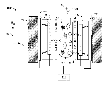
[0028] FIG. 1A is a schematic diagram of an example magnetic resonance system
100.
The example magnetic resonance system 100 shown in FIG. IA includes a primary
magnet system 102, a cooling system 120, a resonator and cavity system 112, a
sample
110 that contains spins 108, a control system 118, a temperature control
system 130,
and a gradient system 140. A magnetic resonance system may include additional
or
different features, and the components of a magnetic resonance system can be
arranged
as shown in FIG. IA or in another manner.
[0029] In the example shown in FIG. 1A, the sample 110 is maintained at a
sample
temperature (Ts). In some implementations, the sample temperature (Ts) is an
ambient
temperature. The temperature control system 130 can provide thermal regulation
that
maintains the sample 110 at a specified temperature. Generally, the sample 110
can be
held at any thermal temperature. In some examples, the sample 110 is a liquid
or
liquid-crystal material, and the sample temperature (Ts) is held at an
appropriate level
to maintain the sample 110 in a liquid state. In some examples, the sample 110
is a live
4
CA 02910747 2015-10-29
WO 2014/176678 PCT/CA2014/000390
imaging subject (e.g., a human or another type of live subject), and the
sample
temperature (Ts) is held at an appropriate level to maintain a desired
environment for
the imaging subject. The temperature control system 130 can use active or
passive
temperature control techniques. For example, the temperature control system
130 may
use a controlled air flow about the sample 110, a heating or cooling element
about the
sample 110, an insulator element about the sample 110, or a combination of
these and
other features to control the temperature of the sample 110.
[00301 In some implementations, the temperature control system 130 includes a
sample temperature controller (STC) unit. The STC unit can include a
temperature
o regulator system that actively monitors the temperature of the sample 110
and applies
temperature regulation. The temperature of the sample 110 can be monitored,
for
example, using a thermocouple to sense the sample temperature. The monitored
temperature information can be used with a feedback system to regulate the
sample
temperature, for example, holding the sample temperature at a specified
constant
value. In some cases, the feedback system can adjust hot or cold air supplied
to the
sample environment by an air supply system. For example, the air supply system
can
include a fan that communicates heated or chilled air into the sample
environment in
response to control data provided by the feedback system.
[0031] The example resonator and cavity system 112 can be used to control the
spin
zo ensemble as described in more detail below. In some cases, the cavity
and resonator
system 112 increases polarization of the spin ensemble by heating or cooling
the spin
ensemble.
[0032] The cooling system 120 provides a thermal environment for the resonator
and
cavity system 112. In some cases, the cooling system 120 can absorb heat from
the
cavity to maintain a low temperature of the cavity. In the example shown in
FIG. 1A,
the cooling system 120 resides in thermal contact with the resonator and
cavity system
112. In some cases, the cooling system 120 maintains the resonator and cavity
system
112 at liquid helium temperatures (e.g., approximately 4 Kelvin), at liquid
nitrogen
temperatures (e.g., approximately 77 Kelvin), or at another cryogenic
temperature
(e.g., less than 100 Kelvin). In some cases, the cooling system 120 maintains
the
resonator and cavity system 112 at pulsed-tube refrigerator temperatures
(e.g., 5 -11
Kelvin), pumped helium cryostat temperatures (e.g., 1.5 Kelvin), helium-3
refrigerator
5
CA 02910747 2015-10-29
WO 2014/176678 PCT/CA2014/000390
temperatures (e.g., 300 milliKelvin), dilution refrigerator temperatures
(e.g., 15
milliKelvin), or another temperature. In some implementations, the temperature
(TO
of the resonator and cavity system 112 is held at or below 10 Kelvin or 100
Kelvin,
while the sample 110 is held above a melting temperature for a material in the
sample
(e.g., a temperature that is above 273 Kelvin for a water-based sample).
[0033] In some cases, the resonator and the cavity are implemented as two
separate
structures, and both are held at the same cryogenic temperature. In some
cases, the
resonator and the cavity are implemented as two separate structures, and the
cavity is
held at a cryogenic temperature while the resonator is held at a higher
temperature. In
o some cases, an integrated resonator/cavity system is held at a cryogenic
temperature.
In general, various cooling systems can be used, and the features of the
cooling system
120 can be adapted for a desired operating temperature Tc, for parameters of
the
resonator and cavity system 112, or for other aspects of the magnetic
resonance system
100.
. Is [0034] In some cases, the magnetic resonance system 100 includes
one or more
thermal barriers that thermally insulate the sample 110 from thermal
interactions with
the colder system components (e.g., components of the cooling system 120,
components of the resonator and cavity system 112, etc.). For instance, the
thermal
barrier can prevent direct contact between the sample 110 and the cooling
system 120,
20 and the thermal barrier can be adapted to reduce indirect heat transfer
between the
sample 110 and the cooling system 120. For example, the temperature control
system
130 can include an insulator that insulates the sample 110 against thermal
interaction
with the cooling system 120. In some implementations, the sample 110 can be
surrounded (e.g., partially or fully surrounded) by a thermal-insulator
material that has
25 low magnetic susceptibility or is otherwise suited to magnetic resonance
applications.
For example, polymide-based plastic materials (e.g., VESPELO manufactured by
DUPONTIlvi) can be used as a thermal barrier between the sample 110 and colder
system components (e.g., the cooling system 120, the resonator and cavity
system 112,
etc.).
30 .. 100351 In general, various cooling systems can be used, and the features
of the cooling
system 120 can be adapted for a desired operating temperature Tc, for
parameters of
the resonator and cavity system 112, or for other aspects of the magnetic
resonance
6
CA 02910747 2015-10-29
WO 2014/176678 PCT/CA2014/000390
system 100. In the example shown in FIG. 1A, the cooling system 120 encloses
the
resonator and cavity system 112 and maintains the temperature Tc of the
resonator and
cavity system 112 below the temperature Ts of sample 110.
[0036] In some implementations, the resonator and cavity system 112 operates
at a
s desired operating temperature Tc that is in the range from room
temperature
(approximately 300 K) to liquid helium temperature (approximately 4 K), and
the
cooling system 120 uses liquid-flow cryostats to maintain the desired
operating
temperature Tc. The cooling system 120 can include an evacuated cryostat, and
the
resonator and cavity system 112 can be mounted on a cold plate inside the
cryostat.
is The resonator and cavity system 112 can be mounted in thermal contact
with the
cryostat, and it can be surrounded by a thermal radiation shield. The cooling
system
120 can be connected to a liquid cryogen source (e.g., a liquid nitrogen or
liquid
helium Dewar) by a transfer line, through which the liquid cryogen can be
continuously transferred to the cold head. The flow rate and liquid cryogen
used can
rs control the operating temperature. Gases can be vented through a vent.
[0037] In some cases, the cooling system 120 uses a closed-loop system (e.g.,
a
commercial Gifford-McMahon pulsed-tube cryo-cooler) to maintain the desired
operating temperature Tc of the resonator and cavity system 112. A closed-loop
or
pulsed-tube system may, in some instances, avoid the need for continuously
20 transferring costly liquid cryogen. In some closed-loop refrigerators,
the cryostat has
two-stages: the first stage (ranging, e.g., from 40 to 80 K) acts as a thermal
insulator
for the second stage, and the second stage encases the cold head and the
resonator and
cavity system 112. Some example closed-loop systems can reach a stable
operating
temperature of 10 Kelvin.
25 [0038] In some cases, the cooling system 120 uses a liquid helium
cryostat to maintain
the desired operating temperature Tc of the resonator and cavity system 112. A
liquid
helium cryostat can be less complicated and more stable in some applications.
When a
liquid helium cryostat is used the resonator and cavity system 112 can be
immersed
(e.g., fully or partially immersed) in liquid helium. The system can include
an outer
30 Dewar that contains liquid nitrogen and an inner Dewar that contains
liquid helium,
and the two Dewars can be separated by a vacuum jacket or another thermal
insulator.
7
CA 02910747 2015-10-29
WO 2014/176678 PCT/CA2014/000390
Liquid helium cryostat systems can typically reach a stable operating
temperature of
approximately 4 Kelvin.
[0039] In some cases, the cooling system 120 uses a helium-gas-flow (or pumped-
helium) cryostat to maintain the desired operating temperature Tc of the
resonator and
cavity system 112. Some commercial helium-gas-flow (or pumped-helium)
cryostats
can reach a stable operating temperature of 1.5 Kelvin. In such cases, the
resonator and
cavity system 112 can be mounted inside the cryostat, and a flow of helium gas
can be
communicated over the surface of the resonator and cavity system 112. In some
implementations, the cooling system 120 includes a liquid helium Dewar that
to surrounds the resonator and cavity system 112 and is thermally isolated
by a vacuum
jacket, and a valve (e.g., a mechanically-controlled needle valve in the
liquid helium
Dewar) can control the flow of helium from the Dewar. The valve can control a
port
that opens into a gas heater, so that the liquid helium is vaporized and flows
to the
resonator and cavity system 112. The valve and heater can be externally
controlled to
is provide the desired temperature regulation.
[0040] Some example helium-gas-flow cryostats can reach operating temperatures
of 1
Kelvin by lowering the vapor pressure of the helium gas in the cryostat. This
can be
achieved by pumping on the helium in a small container (known as the "1-K
pot")
inside the vessel to lower the vapor pressure and thereby lower the boiling
point of
20 liquid helium (e.g., from 4.2 Kelvin down to 1 Kelvin). Some systems can
cool down
even further and reach milliKelvin temperatures, for example, using the helium-
3
isotope (which is generally more expensive than the helium-4 isotope). The
helium-3
can be pumped to much lower vapor pressures, thereby lowering the boiling
point as
low as 200 milliKelvin. A closed-loop system can be used to avoid leaks and
preserve
25 the helium-3 material.
[0041] In some cases, the cooling system 120 uses a dilution refrigerator
system to
maintain the desired operating temperature Tc of the resonator and cavity
system 112.
Dilution refrigerator systems typically use a helium-3 circulation system that
is similar
to the helium-gas-flow cryostat described above. The dilution fridge system
can pre-
30 cool the helium-3 before entering the 1-K pot, to provide an operating
temperature as
low as 2 milliKelvin.
8
CA 02910747 2015-10-29
WO 2014/176678 PCT/CA2014/000390
[0042] The magnetic resonance system 100 shown in FIG. IA can polarize the
spin
ensemble in the sample 110. For example, the magnetic resonance system 100 can
cool
or map the spin ensemble to a thermal equilibrium state or to another state
(i.e., a state
other than the thermal equilibrium state, which may be more polarized or less
s polarized than the thermal equilibrium state). In some cases, the cavity-
based cooling
technique polarizes the spin ensemble to an extent that is determined at least
partially
by the temperature (Tc) of the resonator and cavity system 112.
[0043] In the example shown, the spins 108 in the sample 110 interact
independently
with the primary magnet system 102 and the resonator and cavity system 112.
The
to primary magnet system 102 quantizes the spin states and sets the Larmor
frequency of
the spin ensemble. Rotation of the spin magnetization can be achieved, for
example,
by a radio-frequency magnetic field generated by a resonator. While the spins
are
weakly coupled to the environment, the cavity is well coupled to the
environment (e.g.,
the cooling system 120) so that the time it takes for the cavity to reach
thermal
is equilibrium is much shorter than the time it takes the spins to reach
thermal
equilibrium. The resonator can drive Rabi oscillations in the spin ensemble so
that they
couple to the cavity, and the Dicke states and other angular momenta subspaces
of the
spin system reach thermal equilibrium with the cavity.
[0044] The resonator and cavity system 112 can be described in terms of a
cavity
20 resonance and a spin resonance. The spin resonance is shifted from the
cavity
resonance by the Rabi frequency. The Rabi frequency (i.e., the frequency of
the Rabi
oscillations) can be a function of the power of the drive field applied at the
spin-
resonance frequency. The Rabi frequency can be configured to couple the spins
to the
cavity modes. For example, the power of the drive field can be set such that
the Rabi
25 frequency is substantially equal to the difference between the cavity
resonance and the
spin resonance. In some cases, the system can be modeled as a set of Dicke
states and
angular momenta subspaces of the spin ensemble (i.e., states in the Dicke and
angular
momenta subspace) coupled to the cavity modes through the Tavis-Cummings
Hamiltonian.
30 [0045] A cavity having a low mode volume and high quality factor can
produce a
strong spin-cavity coupling for the spin ensemble. In some instances, the rate
of
photon exchange between the Dicke states and cavity scales as \MI; (the number
of
9
CA 02910747 2015-10-29
WO 2014/176678 PCT/CA2014/000390
spins in the spin ensemble) and g (the spin-cavity coupling strength for a
single spin).
In some examples, the spin-cavity coupling strength is inversely proportional
to the
square root of the mode volume and directly proportional to the square root of
the
admittance (i.e., the quality factor of the cavity).
[0046] In some implementations, the cavity is cooled efficiently and quickly,
and the
heat capacity of the cavity is large compared to the heat capacity of the
spins. In some
instances, the polarization rate produced by the spin-cavity interaction can
be
significantly faster than the thermal T1 relaxation process. In some cases,
the
polarization rate produced by the spin-cavity interaction is faster than any
internal
to relaxation process affecting the spin ensemble, including spontaneous
emission,
stimulated emission, thermal T1 relaxation, or others. For example, as a
result of the
low mode volume and high quality factor cavity, the efficient cavity cooling,
the
efficient spin-cavity coupling, the mixing of angular momenta subspaces or a
combination of these and other features, the spin ensemble can be cooled
quickly
toward the ground state. The mixing of angular momenta subspaces can be
achieved,
for example, by repeating a cavity-cooling process and using an interaction
such as the
Dipolar coupling, natural T2 relaxation, external gradient fields, etc. In
some aspects,
this can provide an effective "short circuit" of the T, relaxation process.
For example,
the technique shown in FIG. 1C can be used to achieve faster spin polarization
in some
instances. In some cases, as a result of the lower temperature of the cavity
(compared
to the higher temperature of the sample), the spin ensemble also reaches a
polarization
that exceeds the thermal equilibrium polarization. Accordingly, in some cases,
the
cavity can increase the polarization at a rate that is faster than the thermal
T1 relaxation
process, and the cavity can produce a higher degree of polarization than the
thermal T,
relaxation process produces.
[0047] FIG. 1C is a flow chart showing an example process 195 for increasing
polarization of a spin ensemble. The example process 195 can be performed, for
example, in the example magnetic resonance system 100 shown in FIG. lA or in
another type of system. The example process 195 shown in FIG. 1C can include
additional or different operations. In some cases, individual operations can
be divided
into multiple sub-operations, or two or more of the operations can be combined
or
performed concurrently as a single operation. Moreover, some or all of the
operations
CA 02910747 2015-10-29
WO 2014/176678 PCT/CA2014/000390
can be iterated or repeated, for example, until a desired state or
polarization is
achieved or until a terminating condition is reached,
[0048] As shown in FIG. 1C, at 196, angular momenta subspaces of a spin
ensemble
are mapped to a lower-energy state. For example, one or more angular momenta
subspaces may be cooled to their respective lowest states. In some cases, a
coherent
interaction between the cavity and the spin ensemble can drive each angular
momentum subspace to its lowest energy state. The mapping can be generated,
for
example, by applying a drive field to the spin ensemble. At 197, the angular
momenta
subspaces are connected. One or more of a number of different techniques can
be used
io to connect the angular momenta subspaces. In some instances, the angular
momenta
subspaces are connected by a process that mixes the various subspaces of the
overall
space. For example, a dipolar interaction among spins, transverse (T2)
relaxation, an
external gradient field, a similar external or internal dephasing interaction,
or a
combination of one or more of these can be used to connect the angular momenta
is subspaces. At 198, a more highly-polarized state is obtained. That is to
say, the state of
the spin ensemble can be more highly polarized than before the spin ensemble's
angular momenta subspaces were cooled to their respective lowest states (at
196) and
connected (at 197). The operations (196, 197) can be iterated one or more
times, for
example, until a desired polarization or other condition is reached.
20 [0049] In some implementations, the initial state of the spin ensemble
(before 196) has
less polarization than the spin ensemble's thermal equilibrium state. For
example, the
initial state of the spin ensemble may be a highly mixed state that has little
or no
polarization. The polarization of the state produced on each iteration can be
higher
than the polarization of the initial state. In some instances, the
polarization is
25 subsequently increased on each iteration. For example, the operations
(196, 197) may
be repeated until the spin ensemble reaches a thermal equilibrium polarization
or
another specified polarization level (e.g., an input polarization for a
magnetic
resonance sequence to be applied to the spin ensemble).
[0050] In some implementations, the process 195 can be used to polarize a spin
30 ensemble on-demand. For example, the process 195 can be initiated at any
time while
the sample is positioned in the magnetic resonance system. In some cases, the
spin
ensemble is polarized between imaging scans or between signal acquisitions.
11
CA 02910747 2015-10-29
WO 2014/176678 PCT/CA2014/000390
Generally, the spin ensemble can be in any state (e.g., any fully or partially
mixed
state) when the process 195 is initiated. In some cases, the process 195 is
initiated on-
demand at a specified time, for example, in a pulse sequence, a spectroscopy
or
imaging process, or another process, by applying the Rabi field for a
specified amount
time.
[00511 In the example shown in FIG. IA, the spin ensemble can be any
collection of
particles having non-zero spin that interact magnetically with the applied
fields of the
magnetic resonance system 100. For example, the spin ensemble can include
nuclear
spins, electron spins, or a combination of nuclear and electron spins.
Examples of
nuclear spins include hydrogen nuclei (1H), carbon-13 nuclei (13C), and
others. In
some implementations, the spin ensemble is a collection of identical spin-1/2
particles.
100521 The example primary magnet system 102 generates a static, uniform
magnetic
field, labeled in FIG. IA and referred here to as the Bo field 104. The
example primary
magnet system 102 shown in FIG. lA can be implemented as a superconducting
solenoid, an electromagnet, a permanent magnet or another type of magnet that
generates a static magnetic field. In FIG. 1A, the example Bo field 104 is
homogeneous over the volume of the sample 110 and oriented along the z
direction
(also referred to here as the "axial direction") of the axisymmetric reference
system
106.
[0053] In some instances, the gradient system 140 generates one or more
gradient
fields. The gradient fields are magnetic fields that spatially vary over the
sample
volume. In some cases, the gradient system 140 includes multiple independent
gradient
coils that can generate gradient fields that vary along different spatial
dimensions of
the sample 110. For example, the gradient system 140 can generate a gradient
field that
varies linearly along the z-axis, the y-axis, the x-axis, or another axis. In
some cases,
the gradient system 140 temporally varies the gradient fields. For example,
the control
system 118 can control the gradient system 140 to produce gradient fields that
vary
over time and space according to an imaging algorithm or pulse program.
[0054] In the example system shown in FIG. 1A, interaction between the spins
108
and the primary magnet system 102 includes the Zeeman Hamiltonian H = -11.= B,
where p. represents the magnetic moment of the spin and B represents the
magnetic
12
CA 02910747 2015-10-29
WO 2014/176678 PCT/CA2014/000390
field. For a spin-1/2 particle, there are two states: the state where the spin
is aligned
with the B, field 104, and the state where the spin is anti-aligned with the
Bo field 104.
With the Bo field 104 oriented along the z-axis, the Zeeman Hamiltonian can be
written H = ¨ 1B0. Quantum mechanically, ft, = yo-z where y is the spin
s gyromagnetic ratio and az is the z-direction spin angular momentum
operator with
angular momentum eigenstates Im), and eignevalues m = +112h, where ft is
Planck's constant.. The factor cos = yBo is the spin-resonance frequency also
known
as the Larmor frequency.
[0055] In the example shown in FIG. 1A, the thermal distribution of individual
it members of the ensemble being either aligned or anti-aligned with the Bo
field 104 is
governed by Maxwell-Boltzmann statistics, and the density matrix for the
thermal
equilibrium state is given by
1 -HlkT
p = ¨ e
where the denominator Z is the partition function, and H is the Hamiltonian of
the spin
is ensemble. The partition function can be expressed Z = , where the sum
is
over all possible spin ensemble configurations. The constant k is the
Boltzmann factor
and T is the ambient temperature. As such, the thermal equilibrium state of
the spin
ensemble (and the associated thermal equilibrium polarization) can be
determined at
least partially by the sample environment (including the magnetic field
strength and
20 the sample temperature), according to the equation above. The
polarization of the spin
ensemble can be computed, for example, from the density matrix representing
the state
of the spin ensemble. In some instances, the spin polarization in the z-
direction can be
computed as the expectation value of the magnetization in the z-direction, Mz,
as
follows:
(Me) = (yh)TrUzP)
(i)
25 where h E Ei=10-z /2 is the total spin ensemble z-angular momentum and
Ns is the
ensemble spin size.
[0056] Once the spin ensemble has thermalized with its environment, any
excitations
that cause deviations away from thermal equilibrium will naturally take time
(characterized by the thermal relaxation rate T1) to thermalize. The thermal
relaxation
13
CA 02910747 2015-10-29
WO 2014/176678 PCT/CA2014/000390
process evolves the spin ensemble from a non-thermal state toward the thermal
equilibrium state at an exponential rate that is proportional to 1/T1. Many
magnetic
resonance applications manipulate the spins and acquire the inductive signals
generated by them. Signal averaging is customarily used to improve the signal-
to-noise
s ratio (SNR). However, the thermal relaxation process takes time, and the
polarization
produced by the thermal relaxation process is limited by the sample
environment
(including the thermal temperature of the sample and the primary magnetic
field
strength). In the example shown in FIG. 1A, the resonator and cavity system
112 can
be used (e.g., in the example process 195 shown in FIG. 1C, or in another
manner) to
io map the spin ensemble to a state that is more polarized than the thermal
equilibrium
state, and in some cases, the resonator and cavity system 112 increases the
spin
ensemble's polarization faster than the thermal relaxation process.
[0057] In some instances, the resonator and cavity system 112 can include a
resonator
component that controls the spin ensemble, and a cavity component that cools
the spin
is ensemble. The resonator and cavity can be implemented as separate
structures, or an
integrated resonator/cavity system can be used. In some implementations, the
resonator is tuned to a resonance frequency of one or more of the spins 108 in
the
sample 110. For example, the resonator can be a radio-frequency resonator, a
microwave resonator, or another type of resonator.
20 [0058] The resonator and cavity system 112 is an example of a multi-mode
resonance
system. In some examples, a multi-mode resonance system has one or more drive
frequencies, one or more cavity modes, and possibly other resonance
frequencies or
modes. The drive frequency can be tuned to the spins' resonance frequency,
which is
determined by the strength of the Bo field 104 and the gyromagnctic ratio of
the spins
25 108; the cavity mode can be shifted from the drive frequency. In some
multi-mode
resonance systems, the drive frequency and the cavity mode are provided by a
single
integrated structure. Examples of integrated multi-mode resonator structures
include
double-loop resonators, birdcage resonators, and other types of structures. In
some
multi-mode resonance systems, the drive frequency and cavity mode are provided
by
30 distinct structures. In some cases, the geometry of a low quality factor
(low-Q) coil can
be integrated with a high-Q cavity such that both the coil and cavity are
coupled to the
14
CA 02910747 2015-10-29
WO 2014/176678 PCT/CA2014/000390
spin system but not to each other. The techniques described here can operate
using a
single drive frequency or possibly multiple drive frequencies applied to the
coil.
[0059] In the example shown in FIG. 1A, the cavity has a resonance frequency
co, that
is different from the resonance frequency of the resonator. The cavity of the
example
resonator and cavity system 112 supports electromagnetic waves whose modes are
determined by physical characteristics of the cavity. Typically, the
fundamental mode
is used as the cavity resonance and the quality factor of the cavity (Q) can
be defined
as the ratio of the stored energy in the cavity mode to the dissipated energy.
In terms of
frequency units, the quality factor of the cavity may be represented
cue
Q
to where co, is the cavity-resonance frequency, and Au) is the -3 dB
bandwidth of the
cavity resonance. In cases where the cavity resonance is given by a
distribution that is
Lorentzian, the bandwidth is given by the full-width at half-maximum (FWHM) of
the
cavity frequency response.
[0060] In some implementations, the cavity of the example resonator and cavity
system 112 has a high quality factor (a high-Q cavity), so that an
electromagnetic field
in the cavity will be reflected many times before it dissipates. Equivalently,
the
photons in the cavity have a long lifetime characterized by the cavity
dissipation rate
K = (CON), where r.i.) is the frequency of the wave. Such cavities can be made
of
superconducting material and kept at cryogenic temperatures to achieve quality
factors
zo that are high in value. For example, the quality factor of a high-Q
cavity can have an
order of magnitude in the range of 10 ¨ 106 or higher. Under these conditions,
the
electromagnetic field in the cavity can be described quantum mechanically as
being
equivalent to a quantum harmonic oscillator: a standard treatment known as
cavity
quantum electrodynamics or cavity QED. This treatment of the electromagnetic
field
in the cavity is in contrast to the Zeeman interaction where only the spin
degree of
freedom is quantum mechanical while the magnetic field is still classical.
[0061] For purposes of illustration, here we provide a quantum mechanical
description
of the cavity modes. Electromagnetic waves satisfy Maxwell's equations and
both the
electric field E and the magnetic field B can be described in terms of a
vector potential
A as
CA 02910747 2015-10-29
WO 2014/176678 PCT/CA2014/000390
B = V x A,
aA
E = .
at
The vector potential itself satisfies the wave equation
a2A
= e2 atr
where c is the speed of light. The wave equation has a formal solution in the
form of
the Fourier series of plane waves:
A =1 (Ak(t) eikr + AL (0 e-ikr),
where each Fourier component Ak(t) also satisfies the wave equation. These
plane
waves are ones that the cavity supports in the case of cavity QED and by
assuming
Ak(t) has time-dependence of the form Ak(t) = Ak el4'kt, the electric and
magnetic
fields are given by
Ek = ICOk(Ak _ AL eicokt-ik.r),
Bk = ik X (Ak _ AL eicokt-ik.r),
where the temporal and spatial frequencies (Wk and k, respectively) are
related by
cok = ck.
[0062] Accordingly, the energy of a single mode k is given by
1
Wk = -2 f dV (cog, + po-1B1c) = 2coVc4 Ak.
where co and po are the permittivity and permeability of free space
respectively, such
that c'poco = 1 and V is the volume of space or cavity containing the
radiation field.
By defining the vector coefficients in terms of a real and imaginary part P
and Q, we
can express Ak as:
Ak = (4coVoik) (wkQk + k )F_k,
where Ek is the polarization vector for the electromagnetic wave. In terms of
Qk and
Pk the energy is given by
16
CA 02910747 2015-10-29
WO 2014/176678 PCT/CA2014/000390
Wk = ¨21 (Pic + wiQD,
which is the form for the energy of a simple harmonic oscillator. Hence, we
may treat
the vectors Qk and Pk of the electromagnetic wave as the position and momentum
vectors of the Harmonic oscillator. This allows us to quantize the
electromagnetic field
in terms of single quanta (photons) by the standard canonical quantization of
the
harmonic oscillator.
[0063] We now consider the quantum treatment of a single electromagnetic mode
in a
cavity. The Hamiltonian for the quantum harmonic oscillator may be written in
terms
of the canonical P and Q variables as
to H= _(p 2
oi2Q2).
2 s'
We may then define operators a and a+, called the annihilation and creation
operators,
respectively, in terms of the vectors P and Q:
a ---
2h to
a+ = (Q ¨ ¨P).
2h
These operators satisfy the commutation relation [a, a+] = 1. Hence, our
Hamiltonian
may be written in terms of the creation and annihilation operators as
1
H = ho) (a+a +.).
t5 The constant factor of a half corresponds to a constant energy shift of
the cavity modes
so we may remove it by going into an interaction frame which rescales the
energies by
this constant amount.
[0064] The energy eigenstates of this Hamiltonian are the so-called number
states,
which correspond to a single quanta (photon) of radiation within the cavity.
They are
zo labeled In), where n = [0, 1, 2,3, ...]. The action of the creation and
annihilation
operators on the number states is to create or remove a photon from the
cavity:
aln), = -1;21n ¨ 1),
aln) ViIn + 1),
17
CA 02910747 2015-10-29
WO 2014/176678 PCT/CA2014/000390
Hence the operator N = a+a (the number operator) gives the total number of
photons
for a given number state:
a+ aln), = nin),.
The photon number state in), is an energy eigenstate of the Hamiltonian
1
liln) =
with energy (n + 12) hur.
s [0065] We now describe how the cavity of the example resonator and cavity
system
112 couples to the spin ensemble containing the spins 108. The dominant
interaction is
once again the spin magnetic dipole coupling to the cavity electromagnetic
fields.
Therefore, we have
HI ..---- ¨g = B,
and now the electromagnetic field of the cavity is treated quantum
mechanically. In
ni terms of the harmonic oscillator operators the magnetic field in the
cavity can be
written as
ha)
B(r,t) = õfp ¨ (a ¨ al.)u(r, t)e-
2V
where c is the propagation direction, yo is the free space permeability
constant, Pt is
the Planck constant, and the function u(r, t) represents the spatial and
temporal wave
behavior. For some examples, we take c = 2, and the function u(r, t) takes the
form
15 u(r, t) = u(r) cos cot = u(y, z) cos kx cos cot, '
where u(y, z) represents the cavity magnetic field spatial profile. In this
form, the
mode volume can be expressed
flu(r)12d3 r
v=
maxnu(r)121.
As such, the mode volume is related to the spatial profile of the cavity
magnetic field,
and higher spatial homogeneity in the cavity magnetic field generally produces
a
20 lower mode volume. The spin-cavity interaction Hamiltonian then becomes
18
CA 02910747 2015-10-29
WO 2014/176678 PCT/CA2014/000390
1
= ¨2 gh(a ¨ at)ax,
where the constant g represents the coupling strength between each spin and
the
cavity, and o is the x-component spin angular momentum operator. The coupling
strength can, in some instances, be defined by the expression
gh = ' i(011311)1 = jii Y2hw iu(r)i =
2V
In the example equations above, the spin-cavity coupling strength is inversely
proportional to the square root of the mode volume.
[0066] The example resonator and cavity system 112 includes a resonator that
can
generate a Rabi field that is applied to the spin ensemble while the sample
resides in
the Bo field 104. For example, the Rabi field can be a continuous field or a
pulsed
to spin-locking field. In combination with the internal Hamiltonian of the
spin system,
the Rabi field can provide universal control of the spin ensemble. In some
implementations, any magnetic resonance experiment or pulse sequence can be
implemented in this manner. The resonator can generate the Rabi field, for
example,
based on signals from the control system 118, and the parameters of the field
(e.g., the
is phase, power, frequency, duration, etc.) can be determined at least
partially by the
signal from the control system 118.
[0067] In the plot 200 shown in FIG. 2, the vertical axis 202 represents the
frequency
response of the resonator and the cavity, the horizontal axis 204 represents a
range of
frequencies, and the curve 206 shows the response shape for an example
20 implementation of the resonator and cavity system 112. In the example
shown, the
lower frequency resonance (labeled cos) is that of the resonator and the
higher
frequency resonance (labeled coc) is that of the cavity. The quality factor
(Q) of the
cavity is higher than the quality factor (Q) of the resonator, and the
resonance
frequencies differ by the Rabi frequency (labeled
25 [0068] The example control system 118 can control the resonator and
cavity system
112 and the gradient system 140 in the magnetic resonance system 100 shown in
FIG.
1A. In some cases, the control system 118 can also control aspects of the
cooling
system 120, the temperature control system 130, or other components of the
magnetic
19
CA 02910747 2015-10-29
WO 2014/176678 PCT/CA2014/000390
resonance system 100. The control system 118 is electrically coupled to, and
adapted
to communicate with, the resonator and cavity system 112. For example, the
control
system 118 can be adapted to provide a voltage or current signal that drives
the
resonator, the cavity, or both; the control system 118 can also acquire a
voltage or
s current signal from the resonator, the cavity, or both.
[00691 When the sample 110 is an imaging subject, the control system 118 can
combine a desired operation with gradient waveforms to generate a magnetic
resonance imaging pulse sequence that manipulates the spins. The pulse
sequence can
be applied, for example, through operation of the resonator and cavity system
112 and
to the gradient system 140, to spatially encode the spin ensemble so that
the received
magnetic resonance signals can be processed and reconstructed into an image.
[00701 FIG. 1B is a schematic diagram of an example control system 150. The
example control system 150 shown in FIG. 1B includes a controller 152, a
waveform
generator 154, and amplifier 156, a transmitter/receiver switch 158, a
receiver 160, a
15 signal processor 162, a gradient waveform generator 164, and gradient
electronics 166.
A control system can include additional or different features, and the
features of a
control system can be configured to operate as shown in FIG. 1B or in another
manner.
[0071] In the example shown in FIG. 1B, the example control system 150 is
adapted to
communicate with an external system 190. For example, the external system 190
can
20 be a resonator, a cavity, or another component of a magnetic resonance
system. The
control system 150 can operate based on inputs provided by one or more
external
sources, including the external system 190 or another external source. For
example, the
control system can receive input from an external computer, a human operator,
or
another source.
25 [0072] The example control system 150 shown in FIG. 1B can operate in
multiple
modes of operation. In a first example mode of operation, the controller 152
provides a
desired control operation 170 to the waveform generator 154. Based on the
desired
control operation 170, the waveform generator 154 generates a waveform 172. In
some
cases, the waveform generator 154 also receives system model data 171, and
uses the
30 system model data 171 to generate the waveform 172. The waveform 172 is
received
by the amplifier 156. Based on the waveform 172, the amplifier 156 generates a
CA 02910747 2015-10-29
WO 2014/176678 PCT/CA2014/000390
transmit signal 174. In this mode of operation, the transmitter/receiver
switch 158 is
configured to output the transmit signal 174 to the external system 190.
[0073] In a second example mode of operation, the transmitter/receiver switch
158 is
configured to acquire a signal from the external system 190. The control
system 150
can amplify, process, analyze, store, or display the acquired signal. As shown
in FIG.
1B, based on the signal acquired from the external system 190, the
transmitter/receiver
switch 158 provides a received signal 176 to the receiver 160. The receiver
160
conditions the received signal 176 and provides the conditioned signal 178 to
the
signal processor 162. The signal processor 162 processes the conditioned
signal 178
and generates data 180. The data 180 is provided to the controller 152 for
analysis,
display, storage, or another action.
[0074] In these and other modes of operation, the controller 152 can also
provide a
desired control operation 182 to the gradient waveform generator 164. Based on
the
desired control operation 182 (which may be the same as, or may be related to,
the
desired control operation 170), the waveform generator 154 generates a
gradient
waveform 184. The gradient electronics 166 generate a gradient control signal
186
based on the gradient waveform 184, and the gradient control signal 186 is
provided to
the external system 190. In some cases, a gradient coil or another device in
the external
system 190 generates a gradient field based on the gradient control signal
186.
[0075] In some cases, the controller 152 includes software that specifies the
desired
control operations 170 and 182 so as to spatially encode a spin ensemble in an
imaging
subject, and the software can construct an image of the imaging subject based
on the
data 180 derived from the received signal 176. The spatial encoding
prescription can
use appropriate magnetic resonance imaging techniques (e.g., typically
including a
Fourier transform algorithm), and the image can be constructed from the
digitized data
by a corresponding decoding prescription (e.g., typically including an inverse
Fourier
transform algorithm).
[0076] The controller 152 can be (or include) a computer or a computer system,
a
digital electronic controller, a microprocessor or another type of data-
processing
apparatus. The controller 152 can include memory, processors, and may operate
as a
general-purpose computer, or the controller 152 can operate as an application-
specific
device.
21
CA 02910747 2015-10-29
WO 2014/176678 PCT/CA2014/000390
[0077] FIG. ID is a schematic diagram of an example magnetic resonance system
100'. The example magnetic resonance system 100' is similar to the magnetic
resonance system 100 shown in FIG. lA and can operate in a similar manner. As
shown in FIG. 113, the sample 110 includes the first group of spins 108 shown
in FIG.
s 1A, and a second group spins 109. The second group of spins 109 can be
the same or
different species as the first group of spins 108. In some cases, each set of
spins resides
in a different material or molecular environment For example, the sample 110
can be a
liquid sample, and the second group of spins 109 can be part of a solute
dissolved in a
solvent that includes the first group of spins 108. As another example, the
sample 110
can be a solid sample, and the second group of spins 109 can be part of a
dilute species
in the environment of an abundant species that includes the first group of
spins 108. In
some cases, the first group of spins 108 can be polarized, for example, as
describe with
respect to FIG. 1A, and the polarization of the first group of spins 108 can
be
transferred to the second group of spins 109.
[0078] For example, spin polarization transfer via cavity-based cooling can
function as
a preparation phase to provide magnetization enhancement before a magnetic
resonance experiment, measurement or imaging is performed. In some
implementations, the enhancement can exceed the enhancement that can be
achieved
using some conventional techniques. The polarization transfer technique may
increase
.. magnetization faster than the thermal relaxation time T1 and give a speed
advantage. In
some cases, cavity-based cooling can be activated on-demand so that
polarization can
be transferred as required.
[0079] In some cases, the first group of spins 108 includes a significantly
larger
number of spins than the second group of spins 109. For example, the number of
spins
in a solvent may be substantially larger (e.g., more than twice as large, an
order of
magnitude larger, etc.) than the number of spins in the solute; the number of
spins in
an abundant species may be substantially larger (e.g., more than twice as
large, an
order of magnitude larger, etc.) than the number of spins in the dilute
species. In some
instances, the rate at which a spin ensemble becomes polarized (e.g., by
cavity-based
cooling techniques) varies according to the number of spins in the ensemble.
For
example, the cooling rate for a spin ensemble of N spins may be proportional
to ViV.
For such cooling techniques, a larger spin ensemble (e.g., a solvent, or an
abundant
22
CA 02910747 2015-10-29
WO 2014/176678 PCT/CA2014/000390
species) can be cooled faster than a smaller spin ensemble (e.g., a solute, or
a dilute
species). Moreover, in some instances, the transfer of polarization from
solvent to
solute is relatively fast, since these are both in the Zeeman manifold.
Therefore, the
ensemble with the lower number of spins (which would cool slower) can now have
the
magnetization of the larger ensemble transferred to it through their dipolar
coupling.
Overall, the polarization and transfer process can be much faster than both
natural
relaxation (e.g., T1 relaxation) and direct cooling of the smaller ensemble.
[0080] FIG. lE is a flow chart of an example process 1000 for transferring
spin
polarization. The example process 1000 can be performed, for example, in the
example
to magnetic resonance system 100' shown in FIG. 1D or in another type of
system. The
example process 1000 shown in FIG. lE can include additional or different
operations.
In some cases, individual operations can be divided into multiple sub-
operations, or
two or more of the operations can be combined or performed concurrently as a
single
operation. Moreover, some or all of the operations can be iterated or
repeated, for
example, until a desired state or polarization is achieved or until a
terminating
condition is reached.
[0081] In the example shown in FIG. 1E, at 1002 the solvent and solute are at
thermal
equilibrium. In some implementations, the process 1000 can be initiated when
the
spins are in another state (i.e., a state other than the thermal equilibrium
state). At
1004, the solvent is polarized to a non-thermal polarization. For example, the
solvent
spins can be polarized above the thermal equilibrium polarization by using the
example techniques described with respect to FIG. 1A.
[0082] At 1006, polarization is transferred from the solvent to the solute.
For example,
all or part of the polarization can be transferred to another spin species or
material
within the sample. In some cases, the polarization is transferred by applying
a pulse
sequence to the solvent spins, the solute spins, or both. For example, the
pulse
sequence can enhance the polarization transfer that arises from the dipolar
interaction
between the solvent and solute spins. The pulse sequence for transferring
polarization
can be applied, for example, by a resonator component of the resonator and
cavity
system 112 or another component of the magnetic resonance system 100' in FIG.
ID.
[0083] In some implementations, with the sample temperature Ts above the
cavity
temperature Tc both solvent and solute will be at thermal equilibrium with
their
23
CA 02910747 2015-10-29
WO 2014/176678 PCT/CA2014/000390
environment at temperature Ts with their respective equilibrium polarization
or
magnetization tlf,(4) and M. In the magnetic field 104 the sample spin energy
levels are
split with energy difference AEA = VA hBo for the abundant spin species and
AED =
yo hB, for the dilute spin species, where IA and ID are their respective
gyromagnetic
ratios.
[0084] In the example shown in FIG. 1E, both spin species are initially at
thermal
equilibrium before the solvent (or abundant spin species) is polarized. After
polarizing
the abundant spin species (e.g., using the cavity-based techniques described
with
respect to FIG. IA), its magnetization has increased, and the spin ensemble is
in a non-
it thermal polarized state. If the sample is liquid, then the magnetization
of the solvent
spin can be transferred to the solute spin, for example, by the Nuclear
Overhauser
Effect (NOE). For example, conventional techniques for transferring
polarization
based on the Nuclear Overhauser Effect can be used. In some instances, the
cross-
relaxation between the solvent and solute spins will transfer solvent
magnetization to
is the solute where the enhancement is given by
AAO,PT MO,CC)
'''D
NIL M
where Mcc is the cavity-cooled magnetization of the solvent spin and Mr is the
solute spin magnetization after polarization transfer to it from the solvent
spin. The
factor n characterizes the coupling and relaxation effects between the two
spin species
and the solute spin interactions with its environment.
20 [0085] When the sample is a solid, the Cross Polarization (CP) technique
can be used.
For example, conventional techniques for transferring polarization based on
Cross
Polarization can be used. Here, we start with the cavity cooled magnetization
NC=cc. of
the abundant spin and flip this magnetization into the transverse plane.
Thereafter,
applying a spin-locking drive field to both spin species such that the
respective Rabi
25 drives are equal (the Hartmann-Hahn condition)
oD
VA L1 Yo
where the Bt and Br are each on resonance with the respective spin species
results in
the transfer of magnetization from the abundant spin to the dilute spin. The
enhancement is proportional to the ratio
24
CA 02910747 2015-10-29
WO 2014/176678 PCT/CA2014/000390
mAo,cc
/t42 =
[0086] We now show an example process by which the spin ensemble (e.g., the
spins
108) in the sample 110 can couple to the cavity and cool under a coherent Rabi
drive.
We start with an inductively driven ensemble of non-interacting spin-1/2
particles
(represented in FIG. IA by the spins 108) quantized in a large static magnetic
field
(represented in FIG. lA by the Bo field 104) and magnetically coupled to a
high-Q
cavity of the resonator and cavity system 112. In the presence of the drive
provided by
the resonator of the resonator and cavity system 112, the spins interact with
the cavity
via coherent radiative processes and the spin-cavity system can be treated
quantum
mechanically as a single collected magnetic dipole coupled to the cavity. In
analogy to
to quantum optics, we describe the spin-cavity dynamics as being generated
by the Tavis-
Cummings (TC) Hamiltonian. Assuming the control field to be on resonance with
the
Larmor frequency of the spins, the spin-cavity Hamiltonian under the rotating-
wave
approximation (RWA) is given by H = Hu + H R (t) 14, with
Ho = (Licata + wsjz,
I R = fIR cos(o)st)Jx, and
= g(atJ_ + af+).
As before, at (a) are the creation (annihilation) operators describing the
cavity, SIR is
the strength of the drive field (Rabi frequency), cd, is the resonant
frequency of the
cavity, cds is the Larmor resonance frequency of the spins, and ,g is the
coupling
strength of the cavity to a single spin in the ensemble in units of h = 1.
Here we have
used the notation that
Ia
= EiNsi 0.a(1)/2
are the total angular momentum spin operators for an ensemble of N, spins. The
state-
space V of a spin ensemble of N, identical spins may be written as the direct
sum of
coupled angular momentum subspaces
Ns
V = 2
0 Venj
J=10
CA 02910747 2015-10-29
WO 2014/176678 PCT/CA2014/000390
where j0 = 0 (1/2) if Ars is even (odd). Vj is the state space of a spin-j
particle with
dimension dj = 2J + 1, and there are nj degenerate subspaces with the same
total
spin/. Since the TC Hamiltonian has a global SU(2) symmetry, it will not
couple
between subspaces in this representation. The largest subspace in this
representation is
called the Dicke subspace and consists of all totally symmetric states of the
spin
ensemble. The Dicke subspace corresponds to a system with total angular
momentum
J = Ars/2. The TC Hamiltonian restricted to the Dicke subspace is known as the
Dicke
model and has been studied for quantum optics.
[0087] The eigenstates of Ho are the tensor products of photon-number states
for the
io cavity and spin states of collective angular momentum of each total-spin
subspace in
the ]5 direction: In),IJ,Inz)s. Here, n = 0,1,2, ..., mz = ¨J, ¨J + 1,...,] ¨
1,1, and J
indexes the coupled angular momentum subspace 1/1. The collective excitation
number
of the joint system is given by Nex = otIct + (Jz +J). The interaction term
1/1
commutes with Alex, and hence preserves the total excitation number of the
system.
is This interaction can drive transitions between the state In), [J, ni,),
and states In +
1) m5 1), and In ¨ 1[J, m5 + 1), at a rate of
+ 1)(g/ + 1) ¨ rriz(mz ¨ 1)) and 1/n(gf + 1) ¨ mz(mz + 1)), respectively.
[0088] After moving into a rotating frame defined by H1 = cos(at a +h), the
spin-
cavity Hamiltonian is transformed to
20 /7(1) e itH, Hscei H1,
Fl(1)= Swat a + SIRJx + g (at j_ + al 4.).
Here, 86) = w ¨ (Ds is the detuning of the drive from the cavity-resonance
frequency,
and we have made the standard rotating wave approximation (RWA) to remove any
time dependent terms in the Hamiltonian.
25 [0089] If we now move into the interaction frame of H2 = &Jetta +
ORJx/2, the
Hamiltonian transforms to
17(2)(t) lionR (t) If_nR H+r1R (t)
H005 (t) = g (e-i5wta eis'tat)J
26
CA 02910747 2015-10-29
WO 2014/176678 PCT/CA2014/000390
= (e-i(6w-aR)t al +(x) ¨ (6('-nR)t (x))
2
H+fiR (t) = ¨ig (e-i(Oto-FnR)tapx) _ e ow+nR)tat j (x))
2
where4x) E jy iJ are the spin-ladder operators in the x-basis.
[0090] In analogy to Hartmann-Hahn matching in magnetic resonance cross-
relaxation
experiments for Sco > 0, we may set the cavity detuning to be close to the
Rabi
frequency of the drive, so that A = Sco ¨ SIT is small compared to Sco. By
making a
second rotating-wave approximation in the interaction Hamiltonian reduces to
the
H_niz flip-flop exchange interaction between the cavity and spins in the x-
basis:
Mt) = 2 (etata4x) ¨ e-latintlix))
This rotating-wave approximation is valid in the regime where the detuning and
Rabi
drive strength are large compared to the time scale, te, of interest (Sr. , 1R
>> 1/tc).
From here we will drop the (x) superscript and just note that we are working
in theJ,
eigenbasis for our spin ensemble.
[0091] In some implementations, isolating the spin-cavity exchange interaction
allows
efficient energy transfer between the two systems, permitting them to relax to
a joint
equilibrium state in the interaction frame of the control field. The coherent
enhancement of the ensemble spin-cavity coupling can enhance spin polarization
in the
angular momenta subspaces IT1 at a rate greatly exceeding the thermal
relaxation rate.
FIG. 3 shows this coherent enhancement in terms of the coupled energy levels
of the
spin-cavity states.
[0092] FIG. 3 shows two example energy level diagrams 302, 304 for a spin
coupled
to a two-level cavity. In both diagrams, the ket 1+0) represents the ground
state of the
spin-cavity system (where the spin and the cavity are in their respective
ground states);
the ket 1-1) represents the excited state of the spin-cavity system (where the
spin and
the cavity are in their respective excited states), and the kets 1+1) and 1-0)
represent
intermediate states. In FIG. 3, the straight arrows represent coherent
oscillations, and
the curved arrows represent cavity dissipation.
27
CA 02910747 2015-10-29
WO 2014/176678 PCT/CA2014/000390
[0093] FIG. 3 shows that when the cavity detuning is matched to the Rabi drive
strength, energy exchange transitions between spin and cavity that cool the
spins are
enhanced. The energy level diagram 302 on the left shows the transitions
produced
without the coherent enhancement provided by the control drive. The energy
level
diagram 304 on the right shows the transition producedwith the coherent
enhancement
provided by the control drive when A = 80.t ¨ 12R is small compared to 5w. As
shown
in the energy level diagram 302 on the left, without the control drive all
transition
pathways are possible. The energy level diagram 304 on the right shows that
when the
Rabi drive is turned on and the cavity detuning is matched to the Rabi
frequency, the
to energy exchange transitions between the spin and cavity that drive the
spins to their
ground state are enhanced.
[0094] In the description below, to model the cavity-induced cooling of the
spin
system, we use an open quantum system description of the cavity and spin
ensemble.
The joint spin-cavity dynamics may be modeled using the time-convolutionless
(TCL)
master equation formalism, allowing the derivation of an effective dissipator
acting on
the spin ensemble alone. Since the spin-subspaces V1 are not coupled by the TC
Hamiltonian, the following derivation is provided for all values off in the
state-space
factorization.
[0095] The evolution of an example spin-cavity system can be described by the
Lindblad master equation
¨dtp(t) = Li(t)p(t) + Dcp(t),
where Lj is the super-operator Li(t)p = p] describing evolution
under the
interaction 14amiltonian and D, is a dissipator describing the quality factor
of the
cavity phenomenologically as a photon amplitude damping channel:
V, = ¨2 ((1 fi)D[a] + fiD [0]).
Here, the function D[A]p) = 2ApAi. ¨ A, p}, ñ= trtataped
characterizes the
temperature of the environment (e.g., the cooling system or other
environment), and
is the cavity dissipation rate (a 1/Q). The expectation value of the number
operator at
equilibrium is related to the temperature T, of the environment by
28
CA 02910747 2015-10-29
WO 2014/176678 PCT/CA2014/000390
= (ewc/kBT ¨ 1)-1 .=> T =(1--)c-[ln (1 nr,
kB /
where kB is the Boltzmann constant.
[0096] The reduced dynamics of the spin ensemble in the interaction frame of
the
dissipator is given to second order by the TCL master equation:
d õ t-to
dt p5(t) = I dr trc[L (t)e'c (t ¨ T)Ps (t) 0 Peg]
where p5(t) -= tr,[p(t)] is the reduced state of the spin ensemble and peg is
the
s equilibrium state of the cavity. Under the condition that lc >> g _INT,
the master
equation reduces to
= J
2 t¨todte_
KI/2(COS(ba-)Dsps(t) ¨ sin (Ar)Ls(t)p (t)),
dt 4 o
where
Ds = (1 + 71)D + u+j,
Lsp = [Ks, P], and
Hs = (1 + fi) J+J_ ¨ J_J+
to are the effective dissipator and Hamiltonian acting on the spin ensemble
due to
coupling with the cavity.
[0097] Under the condition that ic >> WIT. we may take the upper limit of the
integral
in the equation above to infinity to obtain the Markovian master equation for
the
driven spin ensemble:
r
15 ¨dt Ps(t) (n 5L5 s)Ps(t),
2
where
92A g2K
f2, = rs ____
K2 + 4,62 ' K2 + 462.
Here, fisis the frequency of the effective Hamiltonian, and I-, is the
effective
dissipation rate of the spin-system.
29
CA 02910747 2015-10-29
WO 2014/176678 PCT/CA2014/000390
[0098] We can consider the evolution of a spin state that is diagonal in the
coupled
angular momentum basis, p(t) = El Vm.=_ j Pm (Op hm. Here, the sum over./ is
summing over subspaces Vj, and Pl,m(t) = (f,m1p(t)Ij, m) is the probability of
finding the system in the state pf,,,=1],m)(J,ml at time t. In this case the
Markovian
master equation reduces to a rate equation for the populations:
¨ Pi 'm(t) = s 01,77,14P] ,m+i(t) + Bi.mPi,m(t) (t)),
dt
where
ALT?, = (1 + ri)U(/ + 1) ¨ m(m ¨ 1)]
Cj,m = ii[J(1 + 1) ¨ m(m + 1)], and
Bjm = ¨(Am + Cm).
Defining i3j(t) = (PL_J(t), , P j (0), we obtain the following matrix
differential
equation for each subspace
= r5mpo,(0,
dt
where M1 is the tridiagonal matrix
AL_J+1 0 0 0 0 \
BL-1+1 A1,_11.2 0 0 0 1
Mi = 0 CI,..14.1 131,_1+2 241,_14.3 0 =-= 0
\ 0 = 0 C B11!
[0099] For a given state specified by initial populations flj(0), the above
differential
equation has the solution (t) = exp(tr,MJ) Pi (0). The equilibrium state of
each
subspace V1 of the driven spin ensemble satisfies Mj = (co) = 0, and is given
by
pj, eq = Eim.¨/ Pidn( )Pi,n11
where
71m(1 + ñ)¨rn
1'j (m) = (1 + )2J+1 ..... f12J+1.
CA 02910747 2015-10-29
WO 2014/176678 PCT/CA2014/000390
The total spin expectation value for the equilibrium state of the spin
ensemble is
(2] + 1)ii21+1
((Me,¨ ¨1 (1 + 77)2J+1 Ti2J-1-1*
101001 If we consider the totally symmetric Dicke subspace in the limit of N,
>> Ft, we
have that the ground state population at equilibrium is given by P
- Ns/2,¨Ns12
1/(1 + -71) and the final expectation value is approximately (Jõ),q ¨11s/2 +
11.
Thus, the final spin polarization in the Dicke subspace will be roughly
equivalent to
the thermal cavity polarization.
[0101] We note that, if the detuning ow were negative in the example described
above,
matching 1/R = 5w would result in the 1-14aR term being dominant, leading to a
master
equation with the operators]_ and J+ interchanged, the dynamics of which would
drive
to the spin ensemble towards the (J) = J state. The detuning can be made
larger than the
cavity linewidth to prevent competition between the H_aR and 1-1 fin terms,
which
would drive the spin system to a high entropy thermally mixed state.
[0102] In some implementations, the cavity-resonance frequency (toe) is set
below the
spin-resonance frequency (ais) such that the detuning Sco = ¨ at, is a
negative
value. In such cases, the techniques described here can be used to perform
cavity-
based heating of the spins to increase the polarization of spin ensemble. In
such cases,
the energy of the spin ensemble is increased by the interaction between the
cavity and
the spin ensemble.
[0103] The tridiagonal nature of the rate matrix allows -fijj(t) = exp(tr,MJ)
Pj(0) to be
efficiently simulated for large numbers of spins. For simplicity we will
consider the
cooling of the Dicke subspace in the ideal case where the cavity is cooled to
its ground
state (ft = 0), and the spin ensemble is taken to be maximally mixed (i.e.,
P,(0) =-
17 (2] + 1) form = ¨J, ...,J).
101041 FIG. 4 is a plot 400 showing simulated evolution of the normalized
expectation
value of ¨J( t))/] for the Dicke subspace of an example cavity-cooled spin
ensemble. In the plot 400, the vertical axis 402 represents a range of values
of the
normalized expectation value of ¨(Jr (0)/j for the Dicke subspace, and the
horizontal
axis 404 represents a range of time values. In FIG. 4, the expectation values
31
CA 02910747 2015-10-29
WO 2014/176678 PCT/CA2014/000390
represented by the vertical axis 402 are normalized by ¨Ito obtain a maximum
value
of 1, and the time variable represented by the horizontal axis 404 is scaled
by the
effective dissipation rate rs for the spin ensemble.
[0105] The plot 400 includes four curves; each curve represents the simulated
expectation value of (Jx(t)) for the Dicke subspace of a spin ensemble with a
different
number of total spins N2, ranging from N, = 102 to N, = 105. The curve 406a
represents a spin ensemble of 10' spins; the curve 406b represents a spin
ensemble of
103 spins; the curve 406c represents a spin ensemble of 104 spins; and the
curve 406d
represents a spin ensemble of 105 spins.
to [0106] At a value of ¨(1,c(t))/J = 1, the total angular momentum
subspace of the spin
ensemble is completely polarized to the h ground eigenstates As shown in
FIG. 4, the polarization of each spin ensemble increases over time, and the
polarization
increases faster for the larger spin ensembles. For the examples shown, the
three larger
spin ensembles are substantially fully polarized within the timescale shown in
the plot
is 400.
[0107] In some cases, the expectation value (h(t)) versus time can be fitted
to an
exponential to derive an effective cooling time-constant, elf, analogous to
the
thermal spin-lattice relaxation time T1. A fit to a model given by
(4(0) ,
¨ exp (¨
eff
yields the parameters 7'1, eff = 2(2DY/r5 with A = 2.0406 and y = ¨0.9981.
This model
20 includes an exponential rate (1/T1, elf)' analogous to the thermal spin-
lattice relaxation
process, which includes an exponential rate (1/T1). This model can be used for
an
angular momentum subspace (e.g., the Dicke subspace) or the full Hilbert
space. In
some instances, the effective rate (1/T1, eff) is significantly faster than
the thermal rate
(1/T1). An approximate expression for the cooling-time constant for the spin
subspace
25 Vj as a function of is
2 2(K2 + 4A2)
eff(J) = ______
g2K/
32
CA 02910747 2015-10-29
WO 2014/176678 PCT/CA2014/000390
In this effective cooling time-constant, the cooling efficiency is maximized
when the
Rabi drive strength is matched to the cavity detuning (i.e., A = 0). In this
case, the
cooling rate and time-constant simplify to P, = 92/K and T1 elf--- iclg2J,
respectively.
In the case where the cavity is thermally occupied, the final spin
polarization is
roughly equal to the thermal cavity polarization, and for cavity temperatures
corresponding to ff. < -27 the effective cooling constant T1, eff is
approximately equal
to the zero temperature value.
[0108] A magnetic resonance system can be controlled in a manner that
polarizes a
sample at a rate corresponding to the effective cooling constant T1,eff shown
above.
it The magnetic resonance system can be configured according to the
parameters that
adhere to the two rotating wave approximations used to isolate the spin-cavity
exchange term Mt). For implementations where (5a) 12R, the magnetic resonance
system can be configured such that g\r/V-3-<<K<<fIR, << coc, cos.
[0109] For an example implementation using X-band pulsed electron spin
resonance
(ESR) (uic/2rr co5/21r =10 GHz) with samples that contain from roughly N, =
106
spins to N, = 1017 spins, the magnetic resonance system can be configured such
that
fIR/21r =100 MHz, Q = 104 (x/27r = 1 MHz) and g /27r =1 Hz. For these
parameters,
the range of validity of the Markovian master equation is N, <<,2/g2=1012 and
the
Dicke subspace of an ensemble containing roughly 1011 electron spins may be
polarized with an effective T1 of 3.18 us. This polarization time is
significantly shorter
than the thermal T1 for low-temperature spin ensembles, which can range from
seconds to hours.
10110j FIG. 5 is an energy level diagram 500 of an example spin system coupled
to a
cavity. Coherent transitions are denoted by a solid line and cavity
dissipation rates are
denoted by a curved line. States in each subspace Vj are labeled In),I¨J, m)5,
where m is the number of spin excitations and n is the number of cavity
excitations.
Within each subspace 10, for cooling dynamics to appear Markovian, states of
high
cavity excitation number should not be significantly populated on a coarse-
grained
timescale.
[0111] In the examples shown here, the spin ensemble is cooled by a coherent
interaction with the cavity, which increases the polarization of the spin
ensemble.
33
CA 02910747 2015-10-29
WO 2014/176678 PCT/CA2014/000390
These cavity-based cooling techniques are different from thermal T1
relaxation, for
example, because the cavity-based techniques include coherent processes over
the
entire spin ensemble. Thermal T1 relaxation is an incoherent process that
involves
exchanging energy between individual spins and the environment, which is
weakly
coupled when T1 is long. Cavity-based cooling techniques can provide a
controlled
enhancement of the spins' coupling to the thermal environment, by using the
cavity as
a link between the spin ensemble and the environment. The cavity is more
strongly
coupled to the environment than the spin ensemble, so energy in the form of
photons is
dissipated more quickly. Due to the inherently small coupling of an individual
spin to
it the cavity, the cavity can be efficiently coupled to the spin ensemble
by driving the
spin ensemble so that it interacts collectively with the cavity as a single
dipole moment
with a greatly enhanced coupling to the cavity. In some cases, the resulting
link
between the spin ensemble and environment ¨ going through the cavity ¨ is
significantly stronger than the link between the spin ensemble and the
environment in
the absence of the cavity, resulting in higher efficiency of energy
dissipation from the
spin ensemble when using the cooling algorithm, and a shorter effective T1.
[0112] The discussion above shows how the Dicke subspace and the other
subspaces
are polarized by cavity-based cooling techniques. We now describe how the
entire
state can be cooled. Due to a global SU(2) symmetry, the state space of the
spin
zo ensemble factorizes into coupled angular momentum subspaces for the
spins. The
largest dimension subspace is called the Dicke subspace (which corresponds to
an
angular momentum] = N/2, where N is the number of spins). For example:
2 spins: (Spin ¨ /2)02 ¨) Spin ¨ 1 (triplet) e Spin ¨ 0 (singlet)
3 1
3 spins: (Spin ¨ re, ¨) Spin ¨ ¨2 (I) Spin ¨ Spin ¨
2
As shown in FIG. 6, in the 3-spins case, the spin-3/2 subspace has the largest
dimension and thus is the Dicke subspace.
[0113] FIG. 6 is a diagram 600 of an example state space represented as a 3-
spin
Hilbert space. The diagram 600 is a matrix representation of the 3-spin
Hilbert space.
The matrix has a block-diagonal form, where each block along the diagonal
represents
a distinct subspace. The first block represents a spin-3/2 subspace 602, and
the second
and third blocks represent two spin-I/2 subspaces 604a, 604b. In FIG. 6, the
spin-3/2
34
CA 02910747 2015-10-29
WO 2014/176678 PCT/CA2014/000390
subspace 602 is the Dicke subspace because it is the subspace of largest
dimension.
Cavity-based cooling can cool each respective subspace to its respective
ground state.
An interaction that breaks the SU(2) symmetry of the Hilbert space can couple
the
distinct subspaces, and cavity-based cooling can cool the spin system to the
true
ground state of the entire Hilbert space. In the example 3-spins case shown in
FIG. 6,
the true ground state resides in the spin-3/2 subspace 602.
[0114] Cavity-based cooling can act independently on each subspace, cooling
each
subspace to its respective ground state with an effective relaxation time of
1
=
where] is the spin of the subspace, and Fs is the cavity-cooling rate derived
from the
to Markovian master equation. In some examples, the true ground state of
the spin
ensemble is the state where all spins are either aligned or anti-aligned with
the Bo
field, and that state is in the Dicke subspace. Generally, at thermal
equilibrium the spin
ensemble will be in a mixed state, and there will be a distribution of states
populated in
all or substantially all subspaces.
[0115] The true ground state (or in some cases, another state) of the spin
ensemble can
be reached by coupling between the spin-] subspaces. This may be achieved by
an
interaction that breaks the global SU(2) symmetry of the system Hamiltonian,
for
example, as described with respect to FIG. 1C. In some examples, the secular
dipole-
dipole interaction between spins, T2 relaxation, an external gradient field,
or a similar
zo external or internal dephasing interaction is sufficient to break this
symmetry.
[0116] In some implementations, applying the cooling algorithm in the presence
of a
perturbation that breaks this symmetry allows cooling to the true ground
state. In the
case of the dipole-dipole interaction, simulations suggest that the spins can
be cooled
to the true ground state at a factor of approximately .///2 times the cooling
rate of
the Dicke subspace. This gives an effective relaxation time to the true ground
state of
1
dipole = ____________
11\51¨;
CA 02910747 2015-10-29
WO 2014/176678 PCT/CA2014/000390
As in the other examples above, we consider a model that includes an
exponential rate
(1/r1, dipole) that is analogous to the thermal spin-lattice relaxation rate
(1/71).
[0117] FIG. 7 is a plot 700 showing effective cooling times calculated for
example
spin ensembles. The plot 700 includes a log-scaled vertical axis 702 showing a
range
s of cooling times in units of seconds, and a log-scaled horizontal axis
704 showing a
range of values for the number of spins in the spin ensemble AI,. Three curves
are
shown in the plot 700. The curve 708 represents the cooling times for example
spin
ensembles under the thermal T1 relaxation process. The other two curves
represent the
cooling times for the same example spin ensembles under the non-thermal,
coherent,
cavity-based cooling processes described above. In particular, the curve 706a
represents the effective cooling times for a spin ensemble to reach the true
ground
state, and the curve 706b represents the effective cooling times for the Dicke
subspace
to reach its ground state.
[0118] FIG. 7 was generated based on a model of an electron spin ensemble in
an X-
band ESR system. In the model used for these calculations, the resonator and
spin
ensemble are both cooled to liquid helium temperatures (4.2 K). A typical
thermal T1
at this temperature is three seconds for a sample of irradiated quartz. The
thermal T1 is
independent of the number of spins in the sample, as shown by the curve 706a
in FIG.
7.
[0119] To obtain the curve 706b in FIG. 7, showing the effective cooling time
constant
for the Dicke subspace of a sample subjected to cavity-based cooling, we
solved a
Markovian master equation for a spin system having a spin-resonance frequency
of 10
GHz. The model used for the calculations included a cavity-spin coupling of 1
Hz, a
cavity dissipation rate of 1 MHz, a cavity detuning outside the bandwidth of
the
resonator, and a Rabi drive strength equal to this detuning. To obtain the
curve 706a in
FIG. 7, showing the effective cooling time constant for the full spin ensemble
under
cavity-based cooling with dipolar interaction, we based our results on small
numbers
of spins and extrapolated to larger numbers. Our initial findings suggest that
eff Dicke.
36
CA 02910747 2015-10-29
WO 2014/176678 PCT/CA2014/000390
As noted above, we consider a spin polarization model that evolves according
to an
exponential rate (1/T1, eff), which is analogous to the thermal spin-lattice
relaxation
process, which evolves according to an exponential rate (1/T1).
[0120] For the examples shown in FIG. 7, if the sample is initially restricted
to the
Dicke subspace, cavity-based cooling gives a speed up over thermal T1 for
samples of
greater than 105 spins. If we consider a completely mixed sample, by including
a
dipolar interaction while performing cavity-based cooling of the spin
ensemble, we
obtain a speed up over thermal T1 for samples of greater than 1010 spins.
[0121] In the model for cavity-based cooling of a spin ensemble presented
above,
to several assumptions are made for illustration purposes. In some
instances, the results
and advantages described above can be achieved in systems that do not adhere
to one
or more of these assumptions. First, we have assumed that the spin ensemble is
magnetically dilute such that no coupling exists between spins. A spin-spin
interaction
that breaks the global SU(2) symmetry of the Tavis-Cummings (TC) Hamiltonian
will
connect the spin-I subspaces in the coupled angular momentum decomposition of
the
state space. Such an interaction may be used as an additional resource that
should
permit complete polarization of the full ensemble Hilbert space. Second, we
have
neglected the effects of thermal relaxation of the spin system. In some
instances, as the
cooling effect of the cavity on the spin system relies on a coherent spin-
cavity
information exchange, the relaxation time of the spin system in the frame of
the Rabi
drive ¨ commonly referred to as T1,p, ¨ should be significantly longer than
the inverse
cavity dissipation rate 1/1c. Third, we have assumed that the spin-cavity
coupling and
Rabi drive are spatially homogeneous across the spin ensemble. Inhomogeneities
may
be compensated for, for example, by numerically optimizing a control pulse
that
implements an effective spin-locking Rabi drive of constant strength over a
range of
spin-cavity coupling and control field amplitudes.
101221 In some implementations, the ability of the cavity to remove energy
from the
spin system depends at least partially on the cooling power of the cooling
system used
to cool the cavity. In the example simulations presented above, the cooling
power of
the cooling system is taken to be infinite, corresponding to an infinite heat
capacity of
the cavity. The techniques described here can be implemented in a system where
the
37
CA 02910747 2015-10-29
WO 2014/176678 PCT/CA2014/000390
cavity has a finite heat capacity. In FIGS. 8A and 8B, we give a model of the
flow of
entropy and energy in an example cavity-based cooling process.
[0123] FIG. 8A is a schematic diagram 800 showing entropy flow in an example
cavity-based cooling process. In the diagram 800, the spins 802 represent a
spin
ensemble, the cavity 804 represents a cavity that is coupled to the spin
ensemble, for
example, under the conditions described above, and the fridge 806 represents a
refrigerator or another type of cooling system that cools the cavity. Energy
removed
from the spin ensemble flows to the cavity at a rate of rsc, and energy is
removed
from the cavity at a rate of rcF by the (finite) cooling power of the
refrigerator.
[0124] FIG. 8B is a plot 810 showing example values of the dissipation rates
Tic and
ru. The plot 810 includes a vertical axis 812 representing a range of values
for
cooling power in units of microwatts (1.tW), and a log-scaled horizontal axis
814
showing a range of values for the number of spins in the spin ensemble N2.
Because
the cooling power of the fridge 806 is held constant in the simulations
represented in
is the plot 810, the rate ru of entropy removal from the cavity to the
refrigerator remains
constant, as shown by the curve 816a. The rate isc of entropy removal from the
spin
ensemble to the cavity, represented by the curve 816b, was calculated by
specifying
the total energy to be removed from the spin system to polarize it divided by
the time
over which that energy is removed, calculated based on our derived cooling
times. The
total energy removed from the spin system was calculated as (N5/2)hca, where
co was
taken to be 27r10 GHz. In the examples shown, the spin system is an electron
spin
ensemble that starts in the fully mixed state such that half the spins must be
driven to
their ground state.
[0125] Energy deposited into the cavity is removed by the fridge at a rate
that is based
on the cooling power of the fridge, which is typically on the order of tens of
microwatts (as shown in FIG. 8B) in some example applications. The curve 816b
in
FIG. 8B demonstrates that under some conditions, for ensembles larger than
roughly
1013 electron spins, a bottleneck of entropy flow may exist that will limit
the
minimum cooling time for larger ensembles. However, in the example shown, an
ensemble of 10' electron spins may be cooled in roughly 3.18 microseconds (Rs)
given a fridge with cooling power of 50 gW. An ensemble of this size is
sufficient to
obtain a strong electron spin resonance signal.
38
CA 02910747 2015-10-29
WO 2014/176678 PCT/CA2014/000390
[0126] Finally, the derivation of the Markovian master equation above assumes
that no
correlations between cavity and spin system accrue during the cooling process,
such
that there is no back action of the cavity dynamics on the spin system. This
condition
is enforced when the cavity dissipation rate, K, exceeds the rate of coherent
spin-cavity
exchange in the lowest excitation manifold by at least an order of magnitude
(i.e.
109.[). In this Markovian limit, the rate at which spin photons are added to
the
cavity is significantly less than the rate at which thermal photons are added,
meaning
the cooling power of the fridge necessary to maintain the thermal cavity
temperature is
sufficient to dissipate the spin photons without raising the average
occupation number
io of the cavity. From the above equation we see that the cooling
efficiency could be
improved by adding more spins to make K closer to g.1171õ; in this regime the
cooling
power of the fridge may not be sufficient to prevent back action from the
cavity and
non-Markovian effects significantly lower the cooling rate.
[0127] The techniques described above can be implemented in a magnetic
resonance
is imaging (MRI) system and in other environments. FIG. 9 is a schematic
diagram of an
example MRI system 900. The example MM system 900 includes a scanner 910, a
computer system 930 and a sample holder 920 for holding a sample 922. The
sample
holder 920 includes a temperature control system 924 that can regulate the
temperature
of the sample 922. The scanner includes a primary magnet system 912, a
gradient
20 system 914, a cooling system 916, and a resonator and cavity system 918.
An MRI
system can include additional or different features, and the features of an
MRI system
can be arranged as shown in FIG. 9 or in another manner.
[0128] The example primary magnet system 912 is designed to provide a
substantially
constant, homogeneous external magnetic field. For example, the primary magnet
25 system 912 may operate as the primary magnet system 102 shown in FIG.
1A. The
example gradient system 914 includes one or more gradient coils designed to
provide
magnetic field gradients (e.g., gradients along Cartesian axes). For example,
the
gradient system 914 may operate as the gradient system 140 shown in FIG. 1A.
The
gradient fields can be configured to acquire image data of a desired slice or
region of
30 the sample 922, for example, by generating a phase-encoding or slice-
selecting field.
39
CA 02910747 2015-10-29
WO 2014/176678 PCT/CA2014/000390
[0129] The resonator and cavity system 918 can polarize and control a spin
ensemble
in the sample 922. For example, the resonator and cavity system 918 may
operate as
the resonator and cavity system 112 shown in FIG. 1A. The resonator and cavity
system 918 can include a cavity and a resonator, which can be implemented as
an
integrated multi-mode resonator structure or as multiple distinct structures.
The
resonator and cavity system 918 can include radio-frequency coils designed to
transmit
and receive radio-frequency pulses. For example, to acquire an image from the
sample
922, the resonator and cavity system 918 can execute an imaging pulse sequence
in
concert with a gradient sequence executed by the gradient system 914. In some
instances, the resonator and cavity system 918 can include various types of
coils that
can be placed around specific parts of a body (e.g., the head, knee, wrist,
etc.) or be
internally implanted in an imaging subject, depending on the sample and
imaging
applications. In some implementations, the resonator and cavity components
that are
used to polarize the spin ensemble (e.g., as described with respect to FIG.
1A) may
also be used to apply an imaging pulse sequence to the sample 922. In some
implementations, separate radio-frequency coils are used to apply the imaging
pulse
sequence.
[0130] The example cooling system 916 can control the temperature of all or
part of
the resonator and cavity system 918. For example, the cooling system 916 may
operate
zo as the example cooling system 120 shown in FIG. 1A. In some cases, the
cooling
system 916 maintains the cavity, and possibly other components of the
resonator and
cavity system 918, below the temperature of the sample 922. For example, the
cooling
system 916 can provide cooling down to cryogenic temperatures in some
implementations.
[0131] In some instances, the temperature control system 924 regulates the
temperature of the sample 922. For example, temperature control system 924 may
operate as the example temperature control system 130 shown in FIG. 1A. In
some
cases, the temperature control system 924 maintains the sample 922 at room
temperature, or another temperature that is appropriate for an imaging subject
For
example, the imaging subject can be held at liquid-state temperatures, or a
live
imaging subject (e.g., a human) can be held at an appropriate temperature.
CA 02910747 2015-10-29
WO 2014/176678 PCT/CA2014/000390
[0132] In some aspects of operation, the resonator and cavity system 918
interacts
with a spin ensemble (e.g., Hydrogen spins) in the sample 922 to prepare the
spin
ensemble for an imaging scan. In some implementations, the resonator and
cavity
system 918 executes a cavity-based cooling process that brings the spin
ensemble to a
higher level of polarization than the spin ensemble's thermal equilibrium
state (i.e.,
greater than the polarization produced by thermal relaxation in the particular
temperature and magnetic field environment). In some implementations, the
cavity-
based cooling process increases the spin ensemble's polarization at a rate
that is faster
than the thermal T1 relaxation rate. The resulting polarized state of the spin
ensemble
to can be used as an initial state for an imaging scan. After each imaging
scan, the spin
ensemble can be re-polarized for further scans. In some cases, the cavity-
based cooling
process reduces the duration of the imaging process, for example, by reducing
the
number of imaging scans required. In some cases, the cavity-based cooling
process
improves the quality of the image produced, for example, by increasing the
signal-to-
noise ratio of an imaging scan.
[0133] While this specification contains many details, these should not be
construed as
limitations on the scope of what may be claimed, but rather as descriptions of
features
specific to particular examples. Certain features that are described in this
specification
in the context of separate implementations can also be combined. Conversely,
various
features that are described in the context of a single implementation can also
be
implemented in multiple embodiments separately or in any suitable
subcombination.
[0134] Example implementations of several independent, general concepts have
been
described. In one general aspect of what is described above, a drive field is
applied to a
spin ensemble in a static magnetic field. The drive field is adapted to couple
spin states
of the spin ensemble with one or more cavity modes of a cavity. Polarization
of the
spin ensemble is increased by the coupling between the spin states and the
cavity
mode.
[0135] In another general aspect of what is described above, a cavity is
coupled with a
spin ensemble in a sample. The sample can be held at a thermal temperature and
subject to a static magnetic field, and an interaction between the cavity and
the spin
ensemble is generated (e.g., by applying a drive field). The interaction
increases
41
CA 02910747 2015-10-29
WO 2014/176678 PCT/CA2014/000390
polarization of the spin ensemble faster than the internal polarizing process
affecting
the sample.
[0136] In another general aspect of what is described above, a thermal barrier
thermally insulates between a sample and a cavity. The cavity is at a first
temperature,
and the sample is at a second, different temperature. The sample contains a
spin
ensemble in a static magnetic field. An interaction between the cavity and the
spin
ensemble is generated. The interaction increases polarization of the spin
ensemble.
[0137] In another general aspect of what is described above, a magnetic
resonance
imaging (MRI) system includes a cavity adapted to interact with a spin
ensemble in a
it sample in a static magnetic field. The sample is an imaging subject. The
MRI system
includes a resonator adapted to generate an interaction between the cavity and
the spin
ensemble that increases polarization of the spin ensemble. The MRI system can
acquire a magnetic resonance signal from the polarized spin ensemble in the
imaging
subject, and an image of the imaging subject can be generated based on the
magnetic
is resonance signal. In some cases, the imaging subject is held at room
temperature, for
example, at 296 Kelvin, 300 Kelvin, or another appropriate temperature between
290
and 310 Kelvin.
[0138] In another general aspect of what is described above, an interaction
between a
cavity and a first spin ensemble in a sample is generated. The interaction
increases
20 polarization of the first spin ensemble based on a coupling between spin
states of the
first spin ensemble and a cavity mode of the cavity. Polarization is
transferred from the
first spin ensemble to a second spin ensemble in the sample.
[0139] In some implementations of the general concepts described above, the
polarization is transferred from the first spin ensemble to the second spin
ensemble by
25 a dipolar interaction between spins of the respective spin ensembles.
The sample can
be a liquid containing a solvent and a solute; the solvent can be the first
spin ensemble,
and the solute can be the second spin ensemble. Polarization can be
transferred from
the solvent to the solute by a Nuclear Overhauser Effect. The sample can be a
solid
containing an abundant species and a dilute species; the abundant species can
be the
30 first spin ensemble, and the dilute species can be the second spin
ensemble.
Polarization can be transferred from the abundant species to the dilute
species by cross
polarization.
42
CA 02910747 2015-10-29
WO 2014/176678 PCT/CA2014/000390
[0140] In some implementations of the general concepts described above, the
temperature of the cavity is regulated by a cooling system that is thermally
coupled to
the cavity, and the temperature of the sample is regulated by a sample
temperature
control system. The cavity can be maintained at a cryogenic temperature, and
the
sample can be maintained in a liquid state. The cavity can be maintained below
100
Kelvin, and the sample can be maintained above 273 Kelvin (e.g., at room
temperature
or another temperature). In some cases, the thermal barrier inhibits thermal
interaction
between the sample and the cavity.
[0141] In some implementations of the general concepts described above,
polarization
to of the spin ensemble is increased by cavity-based cooling acting
independently on
each angular momentum subspace of the spin ensemble via the coupling between
the
spin states and the cavity mode, and a mixing process mixing the angular
momentum
subspaces. The operations can be applied iteratively in some instances. The
angular
momentum subspaces can be mixed, for example, by a dipolar interaction, a
transverse
is (T2) relaxation process, application of a gradient field, or a
combination of these and
other processes.
[0142] In some implementations of the general concepts described above, the
cavity
has a low mode volume and a high quality factor. The mode volume, the quality
factor,
or a combination of these and other cavity parameters can be designed to
produce a
20 coupling between the spin ensemble and the cavity that effectively
"short-circuits" the
spin ensemble polarization process. In some examples, the cavity has a mode
volume
V and a quality factor Q, such that K >> g jc. Here, N, represents the number
of spins
in the spin ensemble, lc = ()/Q) represents the dissipation rate of the
cavity, w,
represents the resonance frequency of the cavity, and g represents the
coupling
25 strength of the cavity to an individual spin in the spin ensemble. In
some examples, the
dissipation rate K is more than two times grN75. In some examples, the
dissipation rate
K is an order of magnitude greater than g,/i. In some examples, the
dissipation rate lc
is two or three orders of magnitude greater than grIc. In some instances, the
coupling
between the spin ensemble and the cavity increases polarization of the spin
ensemble
30 faster than the thermal spin-lattice (T1) relaxation process.
43
CA 02910747 2015-10-29
WO 2014/176678 PCT/CA2014/000390
101431 In some implementations of the general concepts described above, the
spin
ensemble has a spin-resonance frequency (w,), and the drive field is generated
by a
resonator that is on-resonance with the spin-resonance frequency (6)2). The
drive field
can be a time-varying (e.g., oscillating or otherwise time-varying) magnetic
field. In
some cases, the spin ensemble is a nuclear spin ensemble, and the drive field
is a
radio-frequency field. In some cases, the spin ensemble is an electron spin
ensemble,
and the drive field is a microwave-frequency field.
[0144] In some implementations of the general concepts described above, the
cavity
mode corresponds to a cavity-resonance frequency (we), and the cavity-
resonance
to frequency (we) is detuned from the spin-resonance frequency (w5) by an
amount
Sw = co, ¨ ws. The drive field can have a drive field strength that generates
Rabi
oscillations at a Rabi frequency (flu). In some cases, the detuning So) is
substantially
equal to fIR. For instance, the difference A = 8a) ¨ 11R can be small compared
to the
detuning &a. In some examples, the difference A is less than half the detuning
&v. In
some examples, the difference A is an order of magnitude less than the
detuning 5w. In
some examples, the difference A is two or three orders of magnitude less than
the
detuning Sw.
[0145] In some implementations of the general concepts described above, the
interaction between the cavity and the spin ensemble increases polarization of
the spin
zo ensemble at a polarization rate that is related to a parameter of the
cavity. In some
instances, the polarization rate can be higher or lower due to an
electromagnetic
property of the cavity, such as the value of the quality factor, the value of
the mode
volume, the value of the dissipation rate, or another property.
[0146] In some implementations of the general concepts described above, the
static
magnetic field is applied to the spin ensemble by a primary magnet system, and
the
static magnetic field is substantially uniform over the spin ensemble. The
drive field
can be oriented orthogonal to the static magnetic field. For example, the
static
magnetic field can be oriented along a z-axis, and the drive field can be
oriented in the
xy-plane (which is orthogonal to the z-axis).
[0147] In some implementations of the general concepts described above, the
drive
field is generated by a resonator. In some cases, the resonator and cavity are
formed as
44
CA 02910747 2015-10-29
WO 2014/176678 PCT/CA2014/000390
a common structure or subsystem. For example, the resonator and cavity can be
integrated in a common, multi-mode resonator structure. In some cases, the
resonator
and cavity are formed as two or more separate structures. For example, the
resonator
can be a coil structure having a first resonance frequency, and the cavity can
be a
distinct cavity structure that has a second, different resonance frequency.
The
resonator, the cavity, or both can include superconducting material and other
materials.
[0148] In some implementations of the general concepts described above, the
coupling
between the spin ensemble and the cavity changes the state of the spin
ensemble. For
example, the coupling can map the spin ensemble from an initial (mixed) state
to a
subsequent state that has higher polarization than the initial state. The
subsequent state
can be a mixed state or a pure state. In some cases, the subsequent state has
a purity
that is equal to the purity of the cavity. In some instances, the coupling can
evolve the
spin ensemble from an initial state to the thermal equilibrium state of the
spin
ensemble, or to another state that has higher polarization than the thermal
equilibrium
state. The thermal equilibrium state is typically defined, at least partially,
by the
sample environment (including the sample temperature and the static magnetic
field
strength). In some instances, the coupling can evolve the spin ensemble from
an initial
state to a subsequent state having a polarization that is less than, equal to,
or greater
than the thermal equilibrium polarization.
[0149] In some implementations of the general concepts described above, the
drive
field is adapted to couple the Dicke subspace of the spin ensemble with the
cavity
modes. In some representations of the spin ensemble, the Dicke subspace can be
defined as the largest angular momentum subspace, such that the Dicke subspace
contains all the totally-symmetric states of the spin ensemble. In some
representations,
the Dicke subspace corresponds to a system with total angular momentum] =
N5/2,
where N, is the number of spins in the spin ensemble. In some cases, the Dicke
subspace and multiple other angular momentum subspaces of the spin ensemble
are
coupled with the cavity modes. In some cases, all angular momentum subspaces
of the
spin ensemble are coupled with the cavity modes.
[0150] In some implementations of the general concepts described above, the
interaction between the cavity and the spin ensemble causes the spin ensemble
to
dissipate photons to a thermal environment via the cavity modes. The
interaction can
CA 02910747 2015-10-29
WO 2014/176678 PCT/CA2014/000390
include a coherent radiative interaction between the cavity and the spin
ensemble. In
some cases, the coherent radiative interaction can increase the spin
ensemble's
polarization faster than any incoherent thermal process (e.g., thermal spin-
lattice
relaxation, spontaneous emission, etc.) affecting the spin ensemble. In some
cases, the
interaction drives the spin ensemble so that it interacts collectively with
the cavity as a
single dipole moment.
[0151] A number of embodiments have been described. Nevertheless, it will be
understood that various modifications can be made. Accordingly, other
embodiments
are within the scope of the following claims.
46