Note: Descriptions are shown in the official language in which they were submitted.
MULTISTAGE FULL WAVEFIELD INVERSION PROCESS THAT GENERATES A
MULTIPLE FREE DATA SET
[0001] This paragraph intentionally removed.
FIELD OF THE INVENTION
[0002] Exemplary embodiments described herein pertain generally to the
field of
geophysical prospecting, and more particularly to geophysical data processing.
More
specifically, an exemplary embodiment can include inverting seismic data that
contains
multiple reflections and generating a multiple free data set for use with
conventional seismic
processing.
BACKGROUND
[0003] This section is intended to introduce various aspects of the art,
which may be
associated with exemplary embodiments of the present invention. This
discussion is believed
to assist in providing a framework to facilitate a better understanding of
particular aspects of
the present invention. Accordingly, it should be understood that this section
should be read
in this light, and not necessarily as admissions of prior art.
[0004] Seismic inversion is a process of extracting information about the
subsurface from
data measured at the surface of the Earth during a seismic acquisition survey.
In a typical
seismic survey, seismic waves are generated by a source 101 positioned at a
desired location.
As the source generated waves propagate through the subsurface, some of the
energy reflects
from subsurface interfaces 105, 107, and 109 and travels back to the surface
111, where it is
recorded by the receivers 103. The seismic waves 113 and 115 that have been
reflected in the
subsurface only once before reaching the recording devices are called primary
reflections. In
contrast, multiple reflections 117 and 119 are the seismic waves that have
reflected multiple
times along their travel path back to the surface (dashed lines in Figure 1).
Surface-related
multiple reflections are the waves that have reflected multiple times and
incorporate the
surface of the Earth or the water surface in their travel path before being
recorded.
[0005] As illustrated by Figure 2, the generation of surface-related
multiples requires that
a free surface boundary condition be imposed. Fig. 2 illustrates interbed
multiple 202 and
1
CA 2972033 2018-10-24
CA 02972033 2017-06-22
WO 2016/133561 PCT/US2015/057292
free surface multiple 204. As discussed later in the detailed description
section, the present
technological advancement can remove free surface multiples from a data set.
The dashed
component 206 of the free surface multiple would not occur in the presence of
an absorbing
boundary condition.
[0006] Most seismic inversion methods rely on primary reflections only and
treat all
other seismic modes, including multiple reflections as "noise" that need to be
suppressed
during conventional seismic data processing prior to inversion. There are a
number of
multiple suppression methods available in industry. For example, suppression
methods
include surface-related multiple elimination (SRME), shallow water demultiple
(SWD),
model-based water-layer demultiple (MWD), and predictive deconvolution. Those
of
ordinary skill in the art are familiar with these suppression methods, and
further discussion is
not needed. However, all of the methods struggle with multiple elimination if
the multiple
and primary reflections overlap in the recorded seismic data. Furthermore,
inadequate
application of multiple suppression methods may result in damage to the
primary data,
rendering it unusable for inversion.
[0007] An alternative approach is to use inversion algorithms which accept
the data that
still contain surface-related multiples. Full Wavefield Inversion (FWI) is a
seismic method
capable of utilizing the full seismic record, including the seismic events
that are treated as
"noise" by standard inversion algorithms. The goal of FWI is to build a
realistic subsurface
model by minimizing the misfit between the recorded seismic data and synthetic
(or
modeled) data obtained via numerical simulation.
[0008] FWI is a computer-implemented geophysical method that is used to
invert for
subsurface properties such as velocity or acoustic impedance. The crux of any
FWI
algorithm can be described as follows: using a starting subsurface physical
property model,
synthetic seismic data are generated, i.e. modeled or simulated, by solving
the wave equation
using a numerical scheme (e.g., finite-difference, finite-element etc.). The
term velocity
model or physical property model as used herein refers to an array of numbers,
typically a 3-
D array, where each number, which may be called a model parameter, is a value
of velocity
or another physical property in a cell, where a subsurface region has been
conceptually
divided into discrete cells for computational purposes. The synthetic seismic
data are
compared with the field seismic data and using the difference between the two,
an error or
objective function is calculated. Using the objective function, a modified
subsurface model is
generated which is used to simulate a new set of synthetic seismic data. This
new set of
synthetic seismic data is compared with the field data to generate a new
objective function.
2
This process is repeated until the objective function is satisfactorily
minimized and the
final subsurface model is generated. A global or local optimization method is
used to
minimize the objective function and to update the subsurface model.
[0009] Numerical simulation can generate data with or without free surface
multiples
depending on the boundary condition imposed on top of the subsurface model.
The free
surface boundary condition yields data with surface-related multiples, while
the
transparent (absorbing) boundary condition allows for generation of multiple-
free data.
These two modes of numerical modeling lead to two standard approaches in F WI.
[0010] In one approach, FWI requires that the input seismic data have
undergone some
kind of multiple suppression procedure and uses absorbing boundary condition
to model
multiple-free synthetic data. In the other approach, the data still contain
surface-related
multiples which have to be modeled by imposing a free-surface boundary
condition. The
second approach is preferable, since it saves both time and resources required
by
application of conventional multiple suppression methods. Furthermore, it
ensures that
the integrity of the data is not compromised and has the potential of
extracting additional
information contained in multiple reflections. The drawback of the second
approach is
that it requires accurate modeling of surface-related multiples, which appear
to be
extremely sensitive to errors in the water-bottom reflectivity, source
signature, location,
etc. Even a small mismatch between the measured and simulated multiples may
result in
FWI models that are contaminated by the multiples of strong-contrast
interfaces.
[0011] U.S. Patent 7,974,824 describes the seismic inversion of data
containing
surface-related multiples. Instead of pre-processing seismic data to remove
surface-related
multiples, a seismic waveform inversion process enables comparison of
simulated seismic
data containing surface-related multiples with observed seismic data also
containing
surface-related multiples. Based on this comparing, a model of a subterranean
structure
can be iteratively updated.
[0012] Zhang and Schuster (2013) describes a method where least squares
migration
(LSM) is used to image free-surface multiples where the recorded traces are
used as the
time histories of the virtual sources at the hydrophones and the surface-
related multiples
are the observed data. Zhang D. and Schuster G., "Least-squares reverse time
migration
of multiples," Geophysics, Vol. 79, S11-S21, 2013.
3
CA 2972033 2018-10-24
CA 02972033 2017-06-22
WO 2016/133561 PCT/US2015/057292
SUMMARY
[0013] A method, including: performing, with a computer, a first full
wavefield inversion
process on input seismic data that includes free surface multiples, wherein
the first full
wavefield inversion process is performed with a free-surface boundary
condition imposed on
a top surface of an initial subsurface physical property model, and the first
full wavefield
inversion process generates a final subsurface physical property model;
predicting, with the
computer, subsurface multiples with the final subsurface physical property
model; removing,
with the computer, the predicted subsurface multiples from the input seismic
data;
performing, with the computer, a second full wavefield inversion process on
the input seismic
data with the predicted subsurface multiples removed therefrom, wherein the
second full
wavefield inversion process is performed with an absorbing boundary condition
imposed on a
top surface of an initial subsurface physical property model, and the second
full wavefield
inversion process generates a multiple-free final subsurface physical property
model; and
using the multiple-free final subsurface physical property model as an input
to an imaging or
velocity model building algorithm, or in interpreting a subsurface region for
hydrocarbon
exploration or production.
[0014] In the method, the predicting can include using Born modeling.
[0015] In the method, the Born modeling can include using a background
model and a
reflectivity model.
[0016] The method can further include generating the reflectivity model by
removing the
background model from the intermediate inverted subsurface model by taking a
derivative of
the final subsurface physical property model in a vertical direction.
[0017] The method can include generating the reflectivity model by applying
a filter
operator to the final subsurface physical property model.
[0018] The method can include generating the reflectivity model using a
migration
algorithm.
[0019] In the method, the filter operator is a Butterworth filter in a
wavenumber domain.
[0020] The method can further include removing direct arrivals from the
input seismic
data prior to the Born modeling.
[0021] In the method, the removing can include removing the subsurface
multiples from
the input seismic data with adaptive subtraction.
[0022] The method can further include causing subsurface multiple
reflections generated
by the Born modeling to be free of parasitic events.
4
CA 02972033 2017-06-22
WO 2016/133561 PCT/US2015/057292
[0023] In the method, the Born modeling can be performed with synthetic
data generated
from the final subsurface physical property model on regularly spaced grid
nodes.
[0024] In the method, a length of an interval between the regularly spaced
grid nodes can
be equal to half a distance between seismic receivers in a cross-line
direction.
[0025] Another method, including: performing, with a computer, a first full
wavefield
inversion process on input seismic data that includes free surface multiples,
wherein the first
full wavefield inversion process is performed with a free-surface boundary
condition imposed
on a top surface of an initial subsurface physical property model, and the
first full wavefield
inversion process generates a final subsurface physical property model;
predicting, with the
computer, subsurface multiples with the final subsurface physical property
model;
performing, with the computer, a second full wavefield inversion process on
the input seismic
data, wherein the second wavefield inversion process uses an objective
function that only
simulates primary reflections, the objective function being based on the
predicted subsurface
multiples, and the second full wavefield inversion process generates a
multiple-free final
subsurface physical property model; and using the multiple-free final
subsurface physical
property model as an input to an imaging or velocity model building algorithm,
or in
interpreting a subsurface region for hydrocarbon exploration or production.
[0026] Another method, including: performing, with a computer, a first full
wavefield
inversion process on input seismic data that includes free surface multiples,
wherein the first
full wavefield inversion process is performed with a free-surface boundary
condition imposed
on a top surface of an initial subsurface physical property model, and the
first full wavefield
inversion process generates a final subsurface physical property model;
predicting, with the
computer, subsurface multiples with the final subsurface physical property
model; and
removing, with the computer, the predicted subsurface multiples from the input
seismic data
and preparing multiple-free seismic data.
BRIEF DESCRIPTION OF THE DRAWINGS
[0027] While the present disclosure is susceptible to various modifications
and alternative
forms, specific example embodiments thereof have been shown in the drawings
and are
herein described in detail. It should be understood, however, that the
description herein of
specific example embodiments is not intended to limit the disclosure to the
particular forms
disclosed herein, but on the contrary, this disclosure is to cover all
modifications and
equivalents as defined by the appended claims. It should also be understood
that the drawings
are not necessarily to scale, emphasis instead being placed upon clearly
illustrating principles
CA 02972033 2017-06-22
WO 2016/133561 PCT/US2015/057292
of exemplary embodiments of the present invention. Moreover, certain
dimensions may be
exaggerated to help visually convey such principles.
[0028] Fig. 1 is an example of primary reflections and multiple
reflections.
[0029] Fig. 2 is an example of an interbed surface related multiple and a
free surface
multiple.
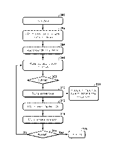
[0030] Fig. 3 is an exemplary flow chart illustrating an embodiment of the
present
technological advancement.
[0031] Fig. 4 is an exemplary flow chart illustrating an embodiment of the
present
technological advancement.
DETAILED DESCRIPTION
[0032] Exemplary embodiments are described herein. However, to the extent
that the
following description is specific to a particular, this is intended to be for
exemplary purposes
only and simply provides a description of the exemplary embodiments.
Accordingly, the
invention is not limited to the specific embodiments described below, but
rather, it includes
all alternatives, modifications, and equivalents falling within the true
spirit and scope of the
appended claims.
[0033] An exemplary embodiment can include inverting seismic data that
contains
multiple reflections and generating a multiple free data set for use with
conventional seismic
processing. In one embodiment, a multi-stage FWI workflow uses multiple-
contaminated
FWI models to predict surface-related multiples with goals of: (1) removing
them from the
data before applying FWI or other inversion or imaging algorithms; and (2)
generating a
multiple free seismic data set for use in conventional seismic data
processing. By way of
example, a method embodying the present technological advancement, can
include: using
data with free surface multiples as input into FWI; generating a subsurface
model by
performing FWT with the free-surface boundary condition imposed on top of the
subsurface
model; using inverted model from FWI to predict multiples; removing predicted
multiples
from the measured data; using the multiple-free data as input into FWI with
absorbing
boundary conditions imposed on top of the subsurface model; and preparing a
multiple free
data set for use in conventional seismic data processing, such as conventional
imaging or
velocity model building algorithms. The present technological advancement
transforms
seismic data into a model of the subsurface.
[0034] Fig. 3 is an exemplary flow chart illustrating an embodiment of the
present
technological advancement. In step 300, the data with free surface multiples
is input into a
6
computer that will apply an FWI workflow to the data with free surface
multiples. The
data with free surface multiples can be a full recorded data set. The data
with free surface
multiples can be obtained by using a source and receivers, as is well known in
the art.
[0035] In step 302, MI is performed on the data with free surface multiples
in the
presence of surface-related multiples. FWI is well-known to those of ordinary
skill in the
art. FWI can utilize an initial geophysical property model, with a free-
surface boundary
condition, and synthetic data can be generated from the initial geophysical
property model.
Generating and/or obtaining synthetic data based on an initial geophysical
property model
is well known to those of ordinary skill in the art. An objective function can
be computed
by using observed geophysical data and the corresponding synthetic data. A
gradient of
the cost function, with respect to the subsurface model parameter(s), can be
used to update
the initial model in order to generate an intermediate model. This iterative
process should
be repeated until the cost function reaches a predetermined threshold, at
which point a
final subsurface physical property model is obtained. Further details
regarding FWI can
be found in U.S. Patent Publication 2011/0194379.
[0036] In step 304, an inverted FWI model (i.e., a subsurface physical
property model)
is generated through the performance of FWI by imposing a free-surface
boundary
condition on top of the initial subsurface model and subsequent revised models
during the
iterative FWI process. In some cases, the inverted FWI model might be
contaminated by
the multiples of the strong-contrast interfaces.
[0037] In step 306, the inverted FWI model is used to predict surface-
related multiples.
To predict surface-related multiples, an approach described in Zhang and
Schuster (2013)
can be used. Assuming that a subsurface model in can be separated into a
slowly varying
(background) component /no and a rapidly varying (reflectivity) component 6m,
the
following equations can be used to predict multiple reflections for the
measured data d(o),
xg, xs) associated with the source at location x, and receivers at locations
xg:
(1)
[V2 -1- (wmo(x))21P(x) d(to, xg,
[V2 + (corno(x))21M(X) W2 2 ont (x)
(2) (1no(x))3
where co is an angular frequency. Equation (1) describes the propagation of
the background
wavefield P(x) through the background model nu. Equation (2) computes the
surface-
7
CA 2972033 2018-10-24
CA 02972033 2017-06-22
WO 2016/133561 PCT/US2015/057292
related multiples M(x) generated when the background wavefield P (x) interacts
with the
reflectivity model dm (see the right-hand side of Equation (2)). The theory
underlying
equations (1)-(2) assumes that seismic data d(co, xfl, xs) is recorded by
receivers positioned
on a dense and regularly spaced grid. Due to the acquisition limitations, both
assumptions are
violated in a typical seismic survey. Irregularities in the acquisition
geometry cause artifacts
in the predicted multiples. The artifacts manifest themselves as parasitic
events that can be
easily mistaken for the real multiple or primary reflections.
10038] In the present embodiment, the measured data (seismic data d) on the
right-hand
side of equation (1) is replaced with synthetic data recorded on a regular and
dense
acquisition geometry. The present embodiment assumes a near-perfect match
between the
measured and synthetic data and requires a model of the subsurface that
ensures such a
match. Advantageously, the present embodiment takes advantage of a subsurface
model built
by applying FWI to the data with free surface multiples (step 304).
10039] There are two approaches to predicting surface related multiples.
Both approaches
require replacing measured data with synthetic data. FWI inverted model is
utilized for this
purpose. Despite the fact that, in some cases, such a model might contain
multiples from
strong contrast interfaces and is not a correct representation of the
subsurface, it is built by
minimizing the mismatch (i.e., cost function) between the measured and
synthetic data.
Therefore, it can generate synthetic data which is a highly accurate
approximation of the
measured data. The first approach is discussed above in regards to Zhang and
Schuster
(2013). The second approach includes the following steps:
1. generate synthetic data using FWI inverted model with free surface boundary
conditions on top of the model;
2. generate synthetic data using FWI inverted model with absorbing boundary
conditions
on top of the model and mirror sources and receivers. Synthetic data generated
with
absorbing boundary conditions contains primary reflections only. Mirror
sources and
receivers ensure that reflections have source and receivers ghosts that match
those of
the data generated in Step 1. Using mirror sources and receivers for
generating source
and receiver ghosts is well known to those of the ordinary skill in the art
and is
discussed, for example, in the patent "Full-wavefield inversion using mirror
source-
receiver geometry"; and
3. subtract synthetic primaries generated in Step 2 from the data generated in
Step 1 to
obtain surface related multiples.
8
[0040] In step 308, predicted multiples are removed from the measured data.
Surface-
related multiples predicted by equations (1)-(2) can be removed from the
measured data
by adaptive subtraction methods. Adaptive subtraction is a method for matching
and
removing coherent noise, such as multiple reflections. Adaptive subtraction
involves a
matching filter to compensate for the amplitude, phase, and frequency
distortions in the
predicted noise model. Conventional adaptive subtraction techniques are known
to those
of ordinary skill in the art and they, for example, can be used to remove the
predicted
multiples in the present embodiment. Examples of adaptive subtraction can be
found, for
example, in Nekut, A. G. and D. J. Verschuur, 1998, Minimum energy adaptive
subtraction
in surface-related multiple attenuation: 68th Ann. Internal Mtg., 1507.1510,
Soc. of Expl.
Geophys., and Neelamani, R., A. Baumstein, and W. S. Ross, 2008, Adaptive
subtraction
using complex curvelet transforms: 70th EAGE Conference and Exhibition, Rome,
G048.
[0041] The resulting multiple-free data (step 310) can be used as an input
into any
inversion algorithm as well as conventional seismic data processing flows.
[0042] Step 312 includes performing a second full wavefield inversion
process on the
input seismic data with the predicted subsurface multiples removed therefrom,
wherein
the second full wavefield inversion process is performed with an absorbing
boundary
condition imposed on a top surface of an initial subsurface physical property
model.
100431 Step 314 includes generating, with the second full wavefield
inversion process,
a multiple-free final subsurface physical property model.
[0044] In step 316, if the acceptance criteria are satisfied, the process
can move to step
318, which can include using the multiple-free final physical property
subsurface model
as an input to a migration algorithm or in interpreting a subsurface region
for hydrocarbon
exploration or production (e.g., drilling a well or imaging the subsurface).
If the
acceptance criteria are not satisfied, the process can return to step 306 for
another
iteration. The acceptance criteria can include having an interpreter examine
the model and
determine if it is acceptable. If the interpreter does not find the model
acceptable,
additional iterations can be executed. Of course, this interpretation by an
interpreter can
be computer assisted with well-known interpretation software.
[0045] In order to create a dense and regular receiver grid required by the
multiple
prediction algorithm implemented in step 306, a bounding box is defined based
on the
minimum and maximum values of the source and receiver locations in the
original
acquisition geometry. The receivers are positioned at regular intervals inside
the bounding
9
CA 2972033 2018-10-24
CA 02972033 2017-06-22
WO 2016/133561 PCT/US2015/057292
box. The length of the interval between the regular grid nodes can be equal to
half the
distance between the receivers in the cross-line direction. Finally, the
geometry is padded
with additional receivers to mitigate artifacts due to the truncation of
receiver lines. The
width of the padding is equal to the length of the taper function used to
gradually force the
recorded wavefield to zero. The original source locations are preserved, since
the multiple
prediction algorithm does not require sources on the regular grid. However, it
is possible to
generate additional data for such multiple suppression algorithms as EPSI,
SRME, etc. A
forward simulation is run using the final FWI model and record the wavefield
at the new
receiver locations.
[0046] Before inserting the recorded wavefields as source functions into
Born modeling
as part of step 306, a taper is applied to the traces recorded by the
receivers located in the
padding zone at the edges of the receiver lines. The purpose of this step is
to ensure that the
subsurface multiple reflections generated by Born modeling are free of the
parasitic events
(e.g., artifacts that can be easily mistaken for the real multiple or primary
reflections). Any
function smoothly varying between 1 and 0 can be used as a taper. One example
of such a
function is Hann window function:
(3) w(n) = 0.5(1 + COS (27Tn)),
where N represent the length of the function in samples and n varies from 0 to
N. Each
sample of the taper function corresponds to the receiver in the padding zone.
About 40
samples are sufficient to force the wavefield in the padding zone to zero.
[0047] The direct arrivals should be removed from the recorded wavefield
prior to
Born modeling. The direct arrivals correspond to the part of the wavefield
that propagates
through the water column from the source to the receivers. In deep water
applications, the
direct arrivals are well separated from the rest of the wavefield and are
typically removed by
muting. In shallow water, the direct arrivals are intermingled with other
seismic events and
cannot be muted without damage to the primary data. This embodiment can make
use of the
known water velocity to model the direct arrival and then subtract it from the
data. After
removing the direct arrivals, a taper is applied to the traces at the edges of
the receiver lines
to gradually force the wavefield to zero.
[0048] Born equations (1)-(2) utilize two subsurface models. The background
model is
smooth and contains only long wavelengths. It can be obtained from tomography,
low
frequency FWI, or by applying a smoothing operator to the final high-frequency
FWI model.
There are several ways to build the reflectivity model. One method includes
removing the
background component from the final FWI model by taking its derivative in the
vertical
direction. Alternatively, the background component can be removed by
application of a filtering
operator to the final FWI model. While both approaches produce a feasible
reflectivity model,
the second approach has the advantage of preserving the reflectivity spectrum
of the original
velocity model. A Butterworth filter (which is a type of signal processing
filter designed to
have as flat frequency response as possible in the passband) can be used in
the wavenumber
domain as the filtering operator, a non-limiting example of which is:
(4) 8(co)2
1+ C7)
where o.) is a wavenumber at which calculation is made, w, is a cut-off
wavenumber, and N is
the length of the filter in samples.
[0049] The choice of the cutoff wavenumber depends on the velocity model
and frequency
of the measured data. For example, for a model that has velocities ranging
from 1500 m/s to
5500 m/s and seismic data with the highest frequency of 40 Hz, the cutoff
wavenumber is 0.005
[0050] The reflectivity model can also be generated using seismic
migration. Migration
algorithms relocate seismic events recorded at the surface of the Earth to the
subsurface location
where the events occurred. The image of the subsurface obtained after
migration of the data
that contains surface related multiples can be used as input into Born
modeling. Kirchhoff
migration is a well-known, cost-efficient and robust way to migrate the data,
however, any
migration algorithm can be used. Seismic Imaging: a review of the techniques,
their principles,
merits and limitations, Etienn Robein Houten, The Netherlands : EAGE
Publications, 2010,
describes a number of migration algorithms that could be used to generate the
reflectivity
model.
[0051] The multiples generated by the Born equations are recorded on the
original
acquisition geometry. Adaptive subtraction is used to remove the multiples
from the measured
data.
[0052] In a second embodiment, instead of removing predicted multiples from
the data, they
are incorporated into FWI. An exemplary way to achieve this is to explicitly
include multiples
into the definition of the objective function. The conventional L2 objective
function is defined
as follows:
(5) E(C) =,iIu_d12,
" 2
11
CA 2972033 2018-10-24
where c is the model of the subsurface and d and u denote observed and
simulated data,
respectively. As mentioned above, inversion of data that contains surface
related multiples can
be challenging due to the mismatch between the measured and simulated
multiples. However,
if the surface related multiples are available prior to the numerical
simulation, it is possible to
design an operator M that accounts for the discrepancies between the simulated
and measured
multiples. In this case, the total simulated data u can be represented as a
sum of primary
reflections uo and surface related multiples u,,,. Then the objective function
requires simulation
of the primary reflections uo only:
( 6) E (c) = Hu() +isrm d112.
[0053] The operator M could be built from a Weiner filter. A Weiner filter
minimizes the
mean square error between the estimated and observed signals. In the present
embodiment, the
estimated signal is predicted multiples, and the observed signal is measured
data. Such Weiner
filters are well known and are described, for example, in Seismic Data
Analysis: Processing,
Inversion and Interpretation of Seismic Data, Oz Yilmaz, Stephen M. Doherty,
Society of
Exploration Geophysicists, 2000.
[0054] Fig. 4 illustrates an exemplary method embodying the present
technological
advancement, where the predicted multiples are incorporated into FWI. Steps
400, 402, 404,
and 406 of Fig. 4 are analogous to steps 300, 302, 304, and 306 of Fig. 3, and
do not need to be
further discussed here.
[0055] A difference between the method of Fig. 3 and the method of Fig. 4
is that the
subtracting step 308 is omitted from the method of Fig. 4, and instead the
second FWI process
uses the predicted multiples as a priori information. Step 408 includes using
multiple-free data
from Step 406 as input into an FWI workflow that uses the modified objective
function
definition and absorbing boundary conditions imposed on top of the subsurface
model.
[0056] Steps 410, 412, and 414 of Fig. 4 are analogous to steps 314, 316,
and 318 of Fig.
3, and do not need to be further discussed here.
[0057] In all practical applications, the present technological advancement
must be used in
conjunction with a computer, programmed in accordance with the disclosures
herein.
Preferably, in order to efficiently perform FWI, the computer is a high
performance computer
(HPC), known as to those skilled in the art. Such high performance computers
typically
involve clusters of nodes, each node having multiple CPU's and computer memory
that allow
12
CA 2972033 2018-10-24
CA 02972033 2017-06-22
WO 2016/133561 PCT/US2015/057292
parallel computation. The models may be visualized and edited using any
interactive
visualization programs and associated hardware, such as monitors and
projectors. The
architecture of system may vary and may be composed of any number of suitable
hardware
structures capable of executing logical operations and displaying the output
according to the
present technological advancement. Those of ordinary skill in the art are
aware of suitable
supercomputers available from Cray or IBM.
10058] The present techniques may be susceptible to various modifications
and
alternative forms, and the examples discussed above have been shown only by
way of
example. However, the present techniques are not intended to be limited to the
particular
examples disclosed herein. Indeed, the present techniques include all
alternatives,
modifications, and equivalents falling within the spirit and scope of the
appended claims.
13