Note: Descriptions are shown in the official language in which they were submitted.
CA 02984894 2017-11-02
WO 2016/209201 PCT/US2015/036947
ACOUSTIC ANISOTROPY USING STATISTICAL ANALYSIS
FIELD OF THE DISCLOSURE
The present disclosure relates generally to downhole logging and, more
specifically, to methods for determining acoustic anisotropy using statistical
analysis of
slowness measurements.
BACKGROUND
The collection of information relating to downhole conditions, commonly
referred
to as "logging," can be performed by several methods including "logging while
drilling"
("LWD") and wireline logging. Downhole acoustic logging tools are often
utilized to
io acquire various characteristics of earth formations traversed by the
borehole. In such
systems, acoustic waveforms are generated using a transmitter, and the
acoustic responses
are received using one or more receiver arrays. The acquired data is then
utilized to
determine the slownesses (velocities) of the formation to obtain a maximum
slowness and
a minimum slowness; and processing the maximum slowness and the minimum
slowness
obtained to determine the horizontal transverse acoustic anisotropy and the
angular
direction of the formation's maximum and minimum slownesses. The amount of
anisotropy and the direction may be of use in well planning and formation
evaluation; for
example, to direct perforation guns or assess wellbore stability.
In order to determine the acoustic anisotropy slowness values, conventional
techniques apply model fitting. In LWD configurations that collect many
slowness
measurements (perhaps 8 or more) randomly in azimuth around the borehole, one
technique fits a periodic model with a cycle period of 180 degrees to these
measurements.
The resulting model's fit phase and amplitude are used to measure the
anisotropy. Also,
wireline logging may use an Alford rotation model to measure anisotropy from
only four
azimuthal slowness measurements, commonly acquired in a "cross-dipole"
configuration.
However, such fitting methods are disadvantageous because the local formation
anisotropy mechanism may be complex and, thus, may deviate from these model
assumptions (in particular that the measured slowness varies sinusoidaly with
azimuth).
Also, a non-random collection of azimuth measurements may bias the model
results,
thereby resulting in inaccurate slowness determinations.
CA 02984894 2017-11-02
WO 2016/209201 PCT/US2015/036947
BRIEF DESCRIPTION OF THE DRAWINGS
FIG. lA illustrates an sonic/acoustic logging tool utilized in an LWD
application,
that acquires slowness measurement signals processed to determine the acoustic
anisotropy
using the illustrative statistical analysis methods described herein;
FIG. 1B illustrates an alternative embodiment of the present disclosure
whereby a
wireline acoustic logging tool acquires and statistically processes the
slowness
measurement signals;
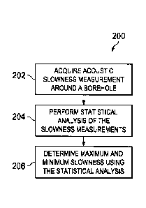
FIG. 2 is a flow chart of a method for determining a maximum and minimum
slowness of a formation using statistical analysis, according to certain
illustrative methods
lo of the present disclosure;
FIG. 3 is a graph of acquired slowness measurements verses their assigned
reference angles relative to the borehole;
FIGS. 4A and 4B are graphs of acquired slowness measurements (stars) wrapped
to
the 0-1800 range and the averaged bin estimates (i.e., characteristic
slovvnesses) (circles)
assuming an 8 bin resolution (FIG. 4A) and a 16 bin resolution (FIG. 4B); and
FIG. 5 is a graph showing the acquired slowness measurements and the
characteristic slowness measurements (bin averages) plotted in a polar
coordinate system,
applying a bifurcation method of the present disclosure.
DESCRIPTION OF ILLUSTRATIVE EMBODIMENTS
Illustrative embodiments and related methodologies of the present disclosure
are
described below as they might be employed in methods and systems to determine
acoustic
anisotropy of a formation using statistical analysis of slowness measurements.
In the
interest of clarity, not all features of an actual implementation or
methodology are
described in this specification. It will of course be appreciated that in the
development of
any such actual embodiment, numerous implementation-specific decisions must be
made to
achieve the developers' specific goals, such as compliance with system-related
and
business-related constraints, which will vary from one implementation to
another.
Moreover, it will be appreciated that such a development effort might be
complex and
time-consuming, but would nevertheless be a routine undertaking for those of
ordinary
skill in the art having the benefit of this disclosure. Further aspects and
advantages of the
various embodiments and related methodologies of the disclosure will become
apparent
from consideration of the following description and drawings.
2
As described herein, illustrative systems and methods of the present
disclosure are
directed to determining acoustic anisotropy of a downholc formation using
statistical
analysis. In a generalized method of the present disclosure, a sonic or
acoustic logging tool
is deployed downhole along a wellbore. Acoustic slowness measurements,
relative to the
formation or borehole coordinates, are then acquired using the logging tool.
Statistical
analysis is performed on the acquired slowness measurements, whereby the
maximum (i.e.,
fast) and minimum (i.e., slow) slownesses (i.e., velocities) and corresponding
angles are
determined. Accordingly, the illustrative methods of the present disclosure
improve the
io sensitivity and detectability of acoustic anisotropy.
Unlike conventional anisotropy techniques, the methods described herein do not
apply model fitting. As previously described, these model fitting techniques
require the
slowness measurement data to be fit into established patterns which may not
resemble the
pattern of a formation's local complex anisotropy mechanisms. In the
illustrative methods
is described herein, however, the slowness measurements are processed using
statistical
analysis to thereby determine the maximum and minimum slownesses of the
formation, as
well as their corresponding angles. In general, statistical analysis uses many
measurements
of an unknown process in order to estimate that process' true properties
directly from the
measurements. As will be described below, the methods of the present
disclosure divide
20 the slowness measurements into groups (referred to herein as "bins"),
whereby the
measurements are averaged, or subjected to other statistical techniques, to
thereby calculate
a characteristic slowness for each bin. These characteristic slownesses are
then compared
to one another using further statistical analysis techniques in order to
determine the
maximum and minimum slownesses and angles. Through use of these statistical
25 techniques, measurement errors are limited which result in a more robust
system.
In yet other methods which further improve angle accuracy, a bifurcation of
the
binned slowness measurements is performed using polar coordinates. As a
result, the
bifurcated measurements are separated into a maximum slowness first azimuthal
angle
range of 90 degrees and a minimum slowness second azimuthal angle range of 90
degrees,
30 which are then statistically analyzed in order to determine the
characteristic maximum and
minimum slowness measurements ¨ from which the maximum and minimum slownesses
and their angles are determined. These and other advantages will be apparent
to those
ordinarily skilled in the art having the benefit of this disclosure.
3
CA 2984894 2019-03-19
CA 02984894 2017-11-02
WO 2016/209201 PCT/US2015/036947
Illustrative methods of the present disclosure may be utilized in a variety of
logging
applications including, for example, LWD or MWD applications. FIG. lA
illustrates an
sonic/acoustic logging tool utilized in an LWD application, that acquires
slowness
measurement signals processed using the illustrative statistical analysis
methods described
herein. The methods described herein may be performed by a system control
center
located on the logging tool or may be conducted by a processing unit at a
remote location,
such as, for example, the surface.
FIG. 1A illustrates a drilling platform 102 equipped with a derrick 104 that
supports
a hoist 106 for raising and lowering a drill string 108. Hoist 106 suspends a
top drive 110
io suitable for rotating drill string 108 and lowering it through well head
112. Connected to
the lower end of drill string 108 is a drill bit 114. As drill bit 114
rotates, it creates a
wellbore 116 that passes through various layers of a formation 118. A pump 120
circulates
drilling fluid through a supply pipe 122 to top drive 110, down through the
interior of drill
string 108, through orifices in drill bit 114, back to the surface via the
annulus around drill
string 108, and into a retention pit 124. The drilling fluid transports
cuttings from the
borehole into pit 124 and aids in maintaining the integrity of wellbore 116.
Various
materials can be used for drilling fluid, including, but not limited to, a
salt-water based
conductive mud.
An acoustic logging tool 126 (also referred to herein as an "acoustic
interrogation
tool") is integrated into the bottom-hole assembly near bit 114. In this
illustrative
embodiment, logging tool 126 is an LWD sonic tool; however, in other
illustrative
embodiments, logging tool 126 may be utilized in a wireline or tubing-conveyed
logging
application. If the logging tool is utilized in an application which did not
rotate the
downhole assembly, the logging tool may be equipped with azimuthally-
positioned sensors
which acquire the slowness measurement around the borehole. In certain other
illustrative
embodiments, acoustic logging tool 126 may be adapted to perform logging
operations in
both open and cased hole environments.
In this example, acoustic logging tool 126 will include multipole-capable
transmitters and receiver arrays (not shown) which generate acoustic waves in
geological
formations and record their transmission. In certain embodiments, the
transmitters may
direct their energies in substantially opposite directions, while in others a
single transmitter
may be utilized and rotated accordingly. The frequency, magnitude, angle and
time of fire
of the transmitter energy may also be controlled, as desired. In other
embodiments, the
4
collected slowness measurements may be stored and processed by the tool
itself, while in
other embodiments the measurements may be communicated to remote processing
circuitry
in order to conduct the statistical processing.
Acoustic logging tool 126 is utilized to acquire slowness measurement data at
many
azimuths. As such, certain embodiments may also include a directional sensor
to
determine the orientation of the tool. The illustrative methods described
herein may be
utilized in a variety of propagation modes, including, for example,
compressional, shear,
flexural, quadrupole or Stoneley modes.
Still referring to FIG. 1A, as drill bit 114 extends wellbore 116 through
formations
o 118,
logging tool 126 collects slowness measurement signals relating to various
formation
properties, as well as the tool orientation and various other drilling
conditions. In certain
embodiments, logging tool 126 may take the form of a drill collar, i.e., a
thick-walled
tubular that provides weight and rigidity to aid the drilling process. A
telemetry sub 128
may be included to transfer slowness images and measurement data/signals to a
surface
is receiver
130 and to receive commands from the surface. In some embodiments, telemetry
sub 128 does not communicate with the surface, but rather stores slowness
measurement
data for later retrieval at the surface when the logging assembly is
recovered.
In certain embodiments, acoustic logging tool 126 includes a system control
center
("SCC"), along with necessary processing/storage/communication circuitry, that
is
20
communicably coupled to one or more transmitters/receivers (not shown)
utilized to
acquire slowness measurement signals. In certain embodiments, once the
slowness
measurement signals are acquired, the system control center calibrates the
signals,
performs the statistical processing methods described herein, and then
communicates the
data back uphole and/or to other assembly components via telemetry sub 128. In
an
25 alternate
embodiment, the system control center may be located at a remote location away
from logging tool 126, such as the surface or in a different borehole, and
performs the
statistical processing accordingly. These and other variations within the
present disclosure
will be readily apparent to those ordinarily skilled in the art having the
benefit of this
disclosure.
30 FIG. 1B
illustrates an alternative embodiment of the present disclosure whereby a
wireline acoustic logging tool acquires and statistically processes the
slowness
measurement signals. At various times during the drilling process, drill
string 108 may be
removed from the borehole as shown in Fig. 1B. Once drill string 108 has been
removed,
5
CA 2984894 2019-03-19
logging operations can be conducted using a wireline acoustic logging sonde
134, i.e., an
acoustic probe suspended by a cable 141 having conductors for transporting
power to the
sonde and telemetry from the sonde to the surface. A wireline acoustic logging
sonde 134
may have pads and/or centralizing springs to maintain the tool near the axis
of the borehole
as the tool is pulled uphole. Acoustic logging sonde 134 can include a variety
of
transmitters/receivers for measuring acoustic anisotropy. A logging facility
143 collects
measurements from logging sonde 134, and includes a computer system 145 for
processing
and storing the slowness measurements gathered by the sensors, as described
herein.
In certain illustrative embodiments, the system control centers utilized by
the
io acoustic logging tools described herein include at least one processor
embodied within
system control center and a non-transitory and computer-readable storage, all
interconnected via a system bus. Software instructions executable by the
processor for
implementing the illustrative statistical processing methods described herein
in may be
stored in local storage or some other computer-readable medium. It will also
be
IS recognized that the statistical processing software instructions may
also be loaded into the
storage from a CD-ROM or other appropriate storage media via wired or wireless
methods.
Moreover, those ordinarily skilled in the art will appreciate that various
aspects of
the disclosure may be practiced with a variety of computer-system
configurations,
including hand-held devices, multiprocessor systems, microprocessor-based or
20 programmable-consumer electronics, minicomputers, mainframe computers,
and the like.
Any number of computer-systems and computer networks are acceptable for use
with the
present disclosure. The disclosure may be practiced in distributed-
computing
environments where tasks are performed by remote-processing devices that are
linked
through a communications network. In a distributed-computing environment,
program
25 modules may be located in both local and/or remote computer-storage
media including
memory storage devices. The present disclosure may therefore, be implemented
in
connection with various hardware, software or a combination thereof in a
computer system
or other processing system.
Now that two illustrative applications of the present disclosure have been
described,
30 a more detailed description of the theory underpinning the present
disclosure will now be
provided. FIG. 2 is a flow chart of a method 200 for determining a maximum and
minimum slowness of a formation using statistical analysis, according to
certain illustrative
methods of the present disclosure. After the acoustic logging tool has been
deployed into a
6
CA 2984894 2019-03-19
CA 02984894 2017-11-02
WO 2016/209201 PCT/US2015/036947
borehole, a number of acoustic slowness measurements are acquired around the
borehole at
block 202. For example, an LWD acoustic tool that is spinning with the bottom
hole
assembly and drill pipe rotation, may take many sonic slowness measurements at
many
angles (in any reference frame desired) while the bottom hole assembly is
drilling, tripping,
circulating, rotating, reaming, etc. The slowness measurements may be acquired
in a
variety of ways, including, for example, using a magnetic azimuth, a north
azimuth, high-
side, or other angle reference, within a short along-hole length (e.g., within
a few inches or
a few seconds). As will be described below, each acoustic acquisition may be
processed
independently to yield an acoustic slowness measurement, which is then paired
with the
reference angle of that same acquisition.
Still referring to block 202, in certain methods the short along-hole length
may be
user-defined. However, in other methods, a computed-optimum along-hole length
is used
to collect neighboring acoustic acquisitions (and their processed
measurements) for
analysis of acoustic anisotropy. For example, all acoustic slowness
measurements within
lft along the hole while the tool (or bottom hole assembly) is spinning and
drilling may be
part of a collection. In certain methods, these collected slowness
measurements may be
displayed using a graph of acquired slowness measurements verses their
assigned reference
angles relative to the borehole, as shown in FIG. 3. DTRS represents the
slowness
measurement ("DT" or delta T) of the refracted shear ("RS") propagation mode.
Note,
however, that other propagation modes may be utilized, as D l'RS is one
example.
Referencing FIG. 3, one illustrative method of the present disclosure may take
slowness measurement from this collection with the slowest (i.e., maximum
slowness
value) slowness and call that measurement's reference angle as the "slow
angle." In FIG.
3, at a depth of 12,155 feet, the maximum slowness would be roughly 185
Its/feet at an
angle of 1500. Similarly, identifying the fastest (i.e., minimum slowness
value) slowness
measurement would give the "fast angle." In FIG. 3, the minimum slowness would
be
roughly 102gs/feet at an angle of 90 . However, dependence on one slowness
measurement each to identify both maximum and minimum slownesses and their
angles for
the formation ignores the other collected measurements shown in FIG. 3.
Moreover, such
a simplified method is subject to measurement errors and may give results that
violate
expected formation acoustic horizontal transverse anisotropy symmetries. The
collected
measurements require further analysis in order to render the acoustic
anisotropy analysis
more robust.
7
CA 02984894 2017-11-02
WO 2016/209201 PCT/US2015/036947
Accordingly, with reference to block 204 of FIG. 2, illustrative methods of
the
present disclosure perform statistical analysis of the acquired slowness
measurements,
thereby limiting errors and providing a more robust analysis. The methods
described
herein assume the measured formation is horizontally transverse isotropic
("HTF) in
relation to the borehole geometry. Therefore, due to either stress or
intrinsic anisotropy of
HTI formations, the slowness measurements around the borehole are symmetrical
by 1800
degrees. In other words, an HTI formation that has a slowness in a given angle
direction
should have that same value of slowness in the angle direction that is 180
from the given
angle.
Therefore, in one illustrative method of block 204, the statistical analysis
is
performed by taking slowness measurements between the 180 and 360 reference
angles,
and subtracting 180 from their reference angles to thereby reassign them into
the 0 to
180' range. Since the distribution of reference slowness angles is usually
random, their
resolution may be regularized by dividing the 0-180 range measurements up
into a
plurality of bins (for example, 8 bins of 22.5 each, or 4 bins of 45 each).
Once the bins
have been generated, each bin's slowness measurements are statistically
analyzed (e.g.,
averaged) to thereby determine a characteristic slowness for each bin. FIGS.
4A and 4B
are graphs of acquired slowness measurements (stars) wrapped to the 0-180
range and the
averaged bin estimates (i.e., characteristic slownesses) (circles) assuming an
8 bin
resolution (4A) and a 16 bin resolution (48). This averaging adds robustness
to the
acoustic anisotropy slowness calculations because single outlier measurements,
like the
one at 150 , do not override the underlying (and possibly unknown) trend of
the data.
Still referring to block 204 of FIG. 2, the illustrative methods described
herein
further assume that an HTI formation's maximum slowness direction is
approximately
perpendicular to the minimum slowness direction. Therefore, this assumption is
applied in
searching for the fastest and slowest bin by analyzing bin slowness
differences. For
example, with reference to FIGS 4A & B, for an 8 bin resolution in a 0-180
range, bins 1
and 5 are 900 degrees (perpendicular) to each other; as are bins 2 and 6, 3
and 7, and 4 and
8. By taking the absolute differences of a bin pair (for example, using the
characteristic
slownesses or combined with other bin statistics, such as bin standard
deviation) for all
pairs, the pair with the largest absolute difference may be identified. This
pair may then be
considered to contain the maximum slowness and minimum slowness measurements
desired for HTI anisotropy identification.
8
Once the bin pair has been determined, the bin with the slower estimated
slowness
is analyzed. In certain methods, the algorithm may use this estimated bin
measurement, or
the slowest actual measurement within the bin, or some other statistical
measurement of the
data to get the desired "slow" or maximum slowness measurement. Similarly, the
.. reference (e.g., middle) angle of the bin, actual measurement within the
bin, or some other
angle estimate may be used to get the desired "slow angle" relative to the
borehole. For
example, the reference angle of FIGS. 4A & B is roughly 900. A similar (but
inverted
logic) may be used to identify the "fast" or minimum slowness measurement and
"fast
angle" from the bin with the fastest estimated slowness. Accordingly, in this
example,
to through comparison of the characteristic slowness measurements, the maximum
and
minimum slowness and their angles relative to the formation are determined at
block 206.
In an alternate method of the present disclosure, bifurcation of the slowness
measurements is utilized to add robustness to the statistical analysis. FIG. 5
is a graph
showing the acquired slowness measurements and the characteristic slowness
measurements (bin averages) plotted in a polar coordinate system. For improved
slowness
angle accuracy, the maximum and minimum slowness angles may be used to
bifurcate the
data into regions for further analysis. By presenting the slowness
measurements versus
angle measurements in a polar representation, where the polar angle is 0-180
degrees and
the polar radius is the slowness measurement, the fast and slow measurements
will
2() naturally group in different 90 degree azimuthal angle ranges (i.e.,
maximum and
minimum slowness 90 degree azimuthal angle ranges) ¨ from which the averaged
bin
estimates (characteristic slowness measurements) are determined. For example,
after
determining the largest absolute difference between characteristic slowness
measurements
of bin pairs (as described above), the initial maximum and minimum slowness
angles are
illustrated in FIG. 5 at ¨ 60 and 150 - which separate the slowness data
into maximum
and minimum 90 degree azimuthal angle ranges.
Using bifurcation lines that are a defined degree (e.g., 45 ) from the
previously
determined fast and slow (bin pair) angles (¨ 60 and 150 ), all or some
(e.g., the
measurements above the mean 90 degree azimuthal angle range slowness) of the
maximum
slowness 90 degree azimuthal angle range measurements can be averaged (e.g.,
using
Cartesian-transformed coordinates to average the measurement points and then
transformed back to angle vs. slowness) to obtain a better maximum slowness
and angle
estimate. In FIG. 5, the bifurcation line is at ¨ 1050 and 15 . Again, all or
some (e.g., the
measurements above or below the mean slowness in the 90 degree azimuthal angle
range)
9
CA 2984894 2019-03-19
of the minimum slowness in 90 degree azimuthal angle range measurements can be
averaged, whereby a refined maximum and minimum slowness angle is determined.
In an
alternative method, the bifurcation line may be used to mirror the data to
confirm the
orientation between fast and slow directions.
Using the statistical processing methods described herein, a full 2D or 3D
image of
the acoustic properties of the borehole may be provided using any variety of
imaging
techniques. Such images may be utilized for a variety of applications,
including, for
example, geosteering of a downhole drilling assembly.
Accordingly, through use of statistical analysis, the illustrative methods of
the
a present disclosure improve the sensitivity and detectability of acoustic
anisotropy acquired
using sonic tools that measure slowness around the borehole.
Embodiments of the present disclosure described herein further relate to any
one or
more of the following paragraphs:
1. A method to determine acoustic anisotropy, comprising acquiring acoustic
15 slowness measurements around a borehole extending along a formation;
performing
statistical analysis on the slowness measurements; and determining a maximum
and
minimum slowness of the formation based upon the statistical analysis.
2. A method as defined in claim paragraph 1, wherein determining the
maximum and minimum slownesses further comprises determining a maximum and
20 minimum slowness angle relative to the borehole.
3. A method as defined in paragraphs 1 or 2, wherein performing the
statistical
analysis comprises grouping the slowness measurements into a plurality of
bins; and
averaging the slowness measurements in each bin to determine a characteristic
slowness
for each bin, wherein the characteristic slowness measurements are compared to
one
25 another in order to determine the maximum and minimum slownesses.
4. A method as defined in any of paragraphs 1-3, further comprising
determining a characteristic maximum and minimum slowness angle relative to
the
borehole; utilizing the characteristic slowness angles to bifurcate the
slowness
measurements of each bin within a polar coordinate system, thereby separating
the
30 slowness measurements into a maximum slowness hemisphere and a minimum
slowness
hemisphere; averaging the slowness measurements in the maximum slowness
hemisphere
to determine a characteristic maximum slowness measurement; and averaging the
slowness
measurements in the minimum slowness hemisphere to determine a characteristic
CA 2984894 2019-03-19
CA 02984894 2017-11-02
WO 2016/209201 PCT/US2015/036947
minimum slowness measurement, thereby determining the maximum and minimum
slownesses.
5. A method as defined in in any of paragraphs 1-4, wherein bifurcating the
slowness measurements further comprises using a bifurcation line positioned at
a defined
degree from the slowness angles.
6. A method as defined in in any of paragraphs 1-5, wherein grouping the
slowness measurements into the plurality of bins comprises assigning a 360
degree
reference angle to each slowness measurement; for those slowness measurements
having
references angles in a 180-360 degree range, subtracting 180 degrees from the
reference
io angles to thereby reassigned those slowness measurements into a 0-180
degree range; and
dividing the slowness measurements in the 0-180 degree range into the
plurality of bins;
and averaging the slowness measurements in each bin further comprises
selecting bin pairs
that are approximately perpendicular to one another; and analyzing each bin
pair to
determine a largest absolute difference in the characteristic slowness
measurements,
thereby determining the maximum and minimum slowrtesses.
7. A method as defined in in any of paragraphs 1-6, wherein the acoustic
slowness measurements are acquired using a rotating acoustic interrogation
tool.
8. A method as defined in any of paragraphs 1-7, wherein the acoustic
slowness measurements are acquired using a stationary acoustic interrogation
tool having
azimuthally-positioned sensors.
9. A method as defined in any of paragraphs 1-8, wherein the acoustic
slowness measurements are acquired using a compressional, shear, flexural,
quadropole or
Stoneley propagation mode.
10. A system to determine acoustic anisotropy, comprising a downhole
assembly comprising at least one transmitter and receiver; and processing
circuitry
communicably coupled to the transmitter and receiver, the processing circuitry
being
configured to implement any of the methods of paragraphs 1-9.
11. A system as defined in paragraph 10, wherein the downhole assembly is a
drilling or wireline assembly.
Moreover, the foregoing paragraphs and other methods described herein may be
embodied within a system comprising processing circuitry to implement any of
the
methods, or a in a computer-program product comprising instructions which,
when
11
CA 02984894 2017-11-02
WO 2016/209201 PCT/US2015/036947
executed by at least one processor, causes the processor to perform any of the
methods
described herein.
Although various embodiments and methods have been shown and described, the
disclosure is not limited to such embodiments and methodologies and will be
understood to
include all modifications and variations as would be apparent to one skilled
in the art.
Therefore, it should be understood that the disclosure is not intended to be
limited to the
particular forms disclosed. Rather, the intention is to cover all
modifications, equivalents
and alternatives falling within the spirit and scope of the disclosure as
defined by the
appended claims.
12