Note: Descriptions are shown in the official language in which they were submitted.
CA 02998522 2018-03-12
WO 2017/058440 PCT/US2016/049392
Q-COMPENSATED FULL WAVEFIELD INVERSION
CROSS-REFERENCE TO RELATED APPLICATIONS
[0001] This application claims the benefit of U.S. Provisional Patent
Application
62/236,190 filed October 2, 2015 entitled Q-COMPENSATED FULL WAVEFIELD
INVERSION, the entirety of which is incorporated by reference herein.
FIELD OF THE INVENTION
[0002] Exemplary embodiments described herein pertain to the field of
geophysical
prospecting, and more particularly to geophysical data processing.
Specifically, embodiments
described herein relate to a method for improving the accuracy of seismic data
by
compensating for subsurface anomalies.
BACKGROUND
[0003] This section is intended to introduce various aspects of the art,
which may be
associated with exemplary embodiments of the present invention. This
discussion is believed
to assist in providing a framework to facilitate a better understanding of
particular aspects of
the present invention. Accordingly, it should be understood that this section
should be read
in this light, and not necessarily as admissions of prior art.
[0004] An important goal of seismic prospecting is to accurately image
subsurface
structures commonly referred to as reflectors. Seismic prospecting is
facilitated by obtaining
raw seismic data during performance of a seismic survey. During a seismic
survey, seismic
energy is generated at ground level by, for example, a controlled explosion,
and delivered to
the earth. Seismic waves are reflected from underground structures and are
received by a
number of sensors referred to as geophones. The seismic data received by the
geophones is
processed in an effort to create an accurate mapping of the underground
environment. The
processed data is then examined with a goal of identifying geological
formations that may
contain hydrocarbons.
[0005] Seismic energy that is transmitted in a relatively vertical
direction into the
earth is the most likely to be reflected by reflectors. Such energy provides
meaningful
information about subsurface structures. However, the seismic energy may be
undesirably
diffused by anomalies in acoustic impedance that routinely occur in the
subsurface
environment. Diffusion of seismic energy during a seismic survey may cause
subsurface
features to be incorrectly represented in the resulting seismic data.
-1-
CA 02998522 2018-03-12
WO 2017/058440 PCT/US2016/049392
[0006] Acoustic impedance is a measure of the ease with which seismic
energy
travels through a particular portion of the subsurface environment. Those of
ordinary skill in
the art will appreciate that acoustic impedance may be defined as a product of
density and
seismic velocity. Acoustic impedance is typically referred to by the symbol Z.
[0007] Seismic waves attenuate for a variety of reasons as they travel in
a subsurface
environment. A quality metric (sometimes referred to a quality factor) Q is
typically used to
represent attenuation characteristics of underground formations. In general, Q
is inversely
proportional to seismic signal attenuation and may range from a value of zero
to infinity.
More specifically, Q is a dimensionless quality factor that is a ratio of the
peak energy of a
wave to the dissipated energy. As waves travel, they lose energy with distance
and time due
to spherical divergence and absorption. Such energy loss must be accounted for
when
restoring seismic amplitudes to perform fluid and lithologic interpretations,
such as amplitude
versus offset (AVO) analysis. Structures with a relatively high Q value tend
to transmit
seismic waves with little attenuation. Structures that tend to attenuate
seismic energy to a
greater degree have lower Q values.
[0008] Q values associated with subsurface structures are used to
mathematically alter
seismic data values to more accurately represent structures in the subsurface
environment.
This process may be referred to as "Q migration" by those of ordinary skill in
the art. During
Q migration, a seismic data value representing travel of seismic energy
through a subsurface
structure having a relatively low Q value may be amplified and broadened in
spectrum to a
greater degree than a data value representing travel of seismic energy through
a subsurface
structure having a relatively high Q value. Altering the amplitude and phase
of data
associated with low Q values takes into account the larger signal attenuation
that occurs when
seismic energy travels through structures having a relatively low Q value.
[0009] FWI is a partial-differential-equation-constrained optimization
method which
iteratively minimizes a norm of the misfit between measured and computed
wavefields.
Seismic FWI involves multiple iterations, and a single iteration can involve
the following
computations: (1) solution of the forward equations, (2) solution of the
adjoint equations, and
(3) convolutions of these forward and adjoint solutions to yield a gradient of
the cost
function. Note that for second-order optimization methods, such as Gauss-
Newton, the (4)
solution of the perturbed forward equations is also required. A more robust
mathematical
justification for this case can be found, for example, in U.S. Patent
Publication
2013/0238246, the entire content of which is hereby incorporated by reference.
-2-
CA 02998522 2018-03-12
WO 2017/058440 PCT/US2016/049392
[0010] A conventional first-order form of the linear visco-acoustic wave
equations for
simulating waves in attenuating acoustic media is:
(3p
- KV = V + EL1011711 = Sp,
ar
av 1,
(1)
ar p
+ kay = v + rpimi = 0,
ar
with appropriate initial and boundary conditions for pressure p, velocity v,
and memory
variables ml. Note that
V = divergence operator,
= = unrelaxed bulk modulus (urn K(w) ¨> K),
(A)¨)C0
= mass density,
= = velocity (v = fvx vy \TAT in 3D space),
= pressure,
m1 = memory variable for mechanism 1,
= = pressure source,
sv = velocity source,
= ¨ and al = (1 ¨ ¨) where relaxation parameters 're/ and TO-1 may be
determined by
Tcyl TEI
equation (2) for a given quality factor profile.
Note that continuous scalar variables are denoted by italicized characters and
vector and
matrices are denoted by bold non-italicized characters throughout this
document.
(4,610o-to-too)
zi=1 2
1+02(r 1(X))
100111 Q-1 (x, w) = _______________________________________________ (2)
yL 1+6)2 TE1(X)Tcrl (X)
z-4=1 2
where
Q = quality factor,
= strain relaxation time of mechanism 1 in SLS model,
= stress relaxation time of mechanism 1 in SLS model,
x = spatial coordinate,
w = frequency,
L = number of relaxation mechanisms used in the SLS model.
-3-
CA 02998522 2018-03-12
WO 2017/058440 PCT/US2016/049392
Conceptually, the quality factor Q represents the ratio of stored to
dissipated energy in a
medium. The strain and stress relaxation times are determined to best fit the
desired quality
factor distribution over the frequency band.
[0012] Full wavefield inversion (FWI) methods based on computing
gradients of an
objective function with respect to the parameters are often efficiently
implemented by using
adjoint methods, which have been proved to outperform other relevant methods,
such as
direct sensitivity analyses, finite differences or complex variable methods.
[0013] The continuous adjoint of the conventional visco-acoustic system
(Equations
(1)) is
v Li = al"
at p) ap'
acral"
¨at + v(Kr) + V(KairTii) =¨' (3)
av
ami
¨at + 0115 =0,
where
15, = adjoint pressure,
V = adjoint velocity,
= adjoint memory variable for mechanism /, and
OF /op and OF /ov are derivatives of the objective function Y with respect to
the pressure
and velocity respectively.
[0014] A common iterative inversion method used in geophysics is cost
function
optimization. Cost function optimization involves iterative minimization or
maximization of
the value of a cost function F(0) with respect to the model 0. The cost
function, also
referred to as the objective function, is a measure of the misfit between the
simulated and
observed data. The simulations (simulated data) are conducted by first
discretizing the
physics governing propagation of the source signal in a medium with an
appropriate
numerical method, such as the finite difference or finite element method, and
computing the
numerical solutions on a computer using the current geophysical properties
model.
[0015] The following summarizes a local cost function optimization
procedure for
FWI: (1) select a starting model; (2) compute a search direction S(0); and (3)
search for an
updated model that is a perturbation of the model in the search direction.
[0016] The cost function optimization procedure is iterated by using the
new updated
model as the starting model for finding another search direction, which will
then be used to
perturb the model in order to better explain the observed data. The process
continues until an
-4-
CA 02998522 2018-03-12
WO 2017/058440 PCT/US2016/049392
updated model is found that satisfactorily explains the observed data.
Commonly used local
cost function optimization methods include gradient search, conjugate
gradients, quasi-
Newton, Gauss-Newton and Newton's method.
[0017]
Local cost function optimization of seismic data in the acoustic approximation
is a common geophysical inversion task, and is generally illustrative of other
types of
geophysical inversion. When inverting seismic data in the acoustic
approximation, the cost
function can be written as:
N N
Efl
Y(0) = Er ENt W (iP õlc( 1 r t wg) ¨ 1P obs(r t, we)), (4)
¨2 g=1 r=1 t=i
where
F(0) = cost function,
0 = vector of N parameters, (Or, 02, ...ON) describing the subsurface
model,
= gather index,
= source function for gather g which is a function of spatial coordinates and
time, for
a point source this is a delta function of the spatial coordinates,
= number of gathers,
= receiver index within gather,
N, = number of receivers in a gather,
= time sample index within a trace,
N t = number of time samples,
= norm function (minimization function, e.g. for least squares function (x) =
x2 ),
Vicalc calculated seismic data from the model 0,
Viobs measured seismic data (pressure, stress, velocities and/or
acceleration).
[0018] The
gathers, data from a number of sensors that share a common geometry,
can be any type of gather (common midpoint, common source, common offset,
common
receiver, etc.) that can be simulated in one run of a seismic forward modeling
program.
Usually the gathers correspond to a seismic shot, although the shots can be
more general than
point sources. For point sources, the gather index g corresponds to the
location of individual
point sources. This generalized source data, yobs can either be acquired in
the field or can
be synthesized from data acquired using point sources. The calculated data uf
on the
= calc
other hand can usually be computed directly by using a generalized source
function when
forward modeling.
-5-
CA 02998522 2018-03-12
WO 2017/058440 PCT/US2016/049392
[0019] FWI
attempts to update the discretized model 0 such that F(0) is a minimum.
This can be accomplished by local cost function optimization which updates the
given model
0(k) as follows:
0 (1+1) = 0 (i) + y (i) S (0 (1)) , (5)
where i is the iteration number, y is the scalar step size of the model
update, and S(0) is the
search direction. For steepest descent, S(0) = ¨V'eF(0), which is the negative
of the
gradient of the misfit function taken with respect to the model parameters. In
this case, the
model perturbations, or the values by which the model is updated, are
calculated by
multiplication of the gradient of the objective function with a step length y,
which must be
repeatedly calculated. For second-order optimization techniques, the gradient
is scaled by the
Hessian (second-order derivatives of objective function with respect to the
model
parameters). The
computation of V'eF(0) requires computation of the derivative
of F(0) with respect to each of the N model parameters. N is usually very
large in
geophysical problems (more than one million), and this computation can be
extremely time
consuming if it has to be performed for each individual model parameter.
Fortunately, the
adjoint method can be used to efficiently perform this computation for all
model parameters
at once (Tarantola, 1984).
[0020] FWI
generates high-resolution property models for prestack depth migration
and geological interpretation through iterative inversion of seismic data
(Tarantola, 1984;
Pratt et al., 1998). With increasing computer resources and recent technical
advances, FWI is
capable of handling much larger data sets and has gradually become affordable
in 3D real
data applications. However, in conventional FWI, the data being inverted are
often treated as
they were collected in an acoustic subsurface medium, which is inconsistent
with the fact that
the earth is always attenuating. When gas clouds exist in the medium, the
quality factor (Q)
which controls the attenuation effect plays an important role in seismic wave
propagation,
leading to distorted phase, dim amplitude and lower frequency. Therefore,
conventional
acoustic FWI does not compensate the Q effect and cannot recover amplitude and
bandwidth
loss beneath gas anomalies.
[0021]
Visco-acoustic FWI, on the other hand, uses both the medium velocity and the
Q values in wave field propagation. Thus, the Q-effect is naturally
compensated while wave-
front proceeds. In some cases, where shallow gas anomalies overlay the
reservoir, severe Q-
effect screens off signals and causes cycle skipping issue in acoustic FWI
implementation.
Consequently, a visco-acoustic FWI algorithm and an accurate Q model are
highly preferred.
-6-
CA 02998522 2018-03-12
WO 2017/058440 PCT/US2016/049392
[0022] The Q values, however, are not easy to determine. Among many
approaches,
ray-based refraction or reflection Q tomography has been largely investigated.
In field data
applications, however, Q tomography is a tedious process and the inversion is
heavily
depending on how to separate attenuated signals from their un-attenuated
counterparts. In
recent years, wave-based inversion algorithms such as FWI have been proposed
to invert for
Q values. Theoretically, such wave-based methods are more accurate. However,
the velocity
and the Q inversion may converge at a difference pace and there might be
severe energy
leakage between velocity and Q gradient so that the inversion results are not
reliable.
[0023] Zhou et al., (2014) describes how to use acoustic FWI for velocity
inversion
and then how to use the FWI inverted velocity model for Q inversion. However,
ray-based Q
tomography is time consuming and they did not conduct a real visco-acoustic
waveform
inversion.
[0024] Bai et al., (2014) applied visco-acoustic FWI for velocity
inversion, however,
they also need to use visco-acoustic FWI to invert for the Q model. As
commonly regarded
by the industry, such a waveform Q inversion is very unstable. The errors in
velocity
inversion may easily leak into Q inversion, and vice versa. In addition, this
method is hard to
do target-oriented Q inversion and Q's resolution and magnitude remain an
issue to be
solved.
SUMMARY
[0025] A method, including: obtaining a velocity model generated by an
acoustic full
wavefield inversion process; generating, with a computer, a variable Q model
by applying
pseudo-Q migration on processed seismic data of a subsurface region, wherein
the velocity
model is used as a guided constraint in the pseudo-Q migration; and
generating, with a
computer, a final subsurface velocity model that recovers amplitude
attenuation caused by
gas anomalies in the subsurface region by performing a visco-acoustic full
wavefield
inversion process, wherein the variable Q model is fixed in the visco-acoustic
full wavefield
inversion process.
[0026] The method can further include generating a subsurface image based
on the
final subsurface velocity model.
[0027] The method can further include: generating the processed seismic
data,
wherein the generating includes applying an acoustic ray-based pre-stack depth
migration to
the velocity model and outputting common image gathers.
[0028] In the method, the generating the variable Q model includes
flattening the
common image gathers in accordance with the guided constraint.
-7-
CA 02998522 2018-03-12
WO 2017/058440 PCT/US2016/049392
[0029] In the method, the guided constraint defines a zone, within the
velocity model,
that contains a gas anomaly.
[0030] In the method, the pseudo Q migration is only applied to the zone
that contains
the gas anomaly.
[0031] In the method, the variable Q model is kept fixed through an
entirety of the
visco-acoustic full wavefield inversion process.
[0032] In the method, the generating the final subsurface velocity model
includes
applying pseudo-Q migration to construct another variable Q model via
flattening visco-
acoustic common image gathers, and the velocity model generated from the visco-
acoustic
full wavefield inversion process is used as a guided constraint in the pseudo-
Q migration.
[0033] The method can further include iterative repeating, until a
predetermined
stopping condition is reached, performance of the visco-acoustic full
wavefield inversion
process, then generation of visco-acoustic common image gathers from visco-
acoustic ray-
based pre-stack depth migration, and then generation of another variable Q
model via
flattening the visco-acoustic common image gathers, wherein the velocity model
generated
from the visco-acoustic full wavefield inversion process is used as a guided
constraint in the
pseudo-Q migration.
[0034] The method can further include conducting a seismic survey,
wherein at least
one source is used to inject acoustic signals into the subsurface and at least
one receiver is
used to record the acoustic signals reflecting from subsurface features.
[0035] The method can further include using the final subsurface velocity
model and
the image of the subsurface to extract hydrocarbons.
[0036] The method can further include drilling a well to extract the
hydrocarbons,
wherein the well is disposed at a location determined by analysis of the
subsurface image.
[0037] In the method, the guided constraint is guided by geological
structures
inverted from the acoustic full wavefield inversion process.
BRIEF DESCRIPTION OF THE DRAWINGS
[0038] While the present disclosure is susceptible to various
modifications and
alternative forms, specific example embodiments thereof have been shown in the
drawings
and are herein described in detail. It should be understood, however, that the
description
herein of specific example embodiments is not intended to limit the disclosure
to the
particular forms disclosed herein, but on the contrary, this disclosure is to
cover all
modifications and equivalents as defined by the appended claims. It should
also be
-8-
CA 02998522 2018-03-12
WO 2017/058440 PCT/US2016/049392
understood that the drawings are not necessarily to scale, emphasis instead
being placed upon
clearly illustrating principles of exemplary embodiments of the present
invention. Moreover,
certain dimensions may be exaggerated to help visually convey such principles.
[0039] Fig. 1 is a graphical representation of a subsurface region that
is useful in
explaining the operation of an exemplary embodiment of the present invention
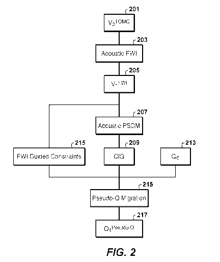
[0040] Fig. 2 illustrates an exemplary method of generating a starting
velocity model
and starting Q model.
[0041] Fig. 3 illustrates an exemplary method of visco-acoustic FWI.
[0042] Fig. 4A illustrates an exemplary velocity model.
[0043] Fig. 4B illustrates an exemplary Q model to match a gas cloud in
Fig. 4A.
[0044] Fig. 5A illustrates exemplary common offset data generated by
acoustic
forward modeling.
[0045] Fig. 5B illustrates exemplary common offset data generated by
visco-acoustic
forward modeling.
[0046] Fig. 6A illustrates an exemplary velocity update generated from
acoustic FWI.
[0047] Fig. 6B illustrates an exemplary velocity update generated from
visco-acoustic
FWI with Q values fixed.
DETAILED DESCRIPTION
[0048] Exemplary embodiments are described herein. However, to the extent
that the
following description is specific to a particular embodiment, this is intended
to be for
exemplary purposes only and simply provides a description of the exemplary
embodiments.
Accordingly, the invention is not limited to the specific embodiments
described below, but
rather, it includes all alternatives, modifications, and equivalents falling
within the true spirit
and scope of the appended claims.
[0049] Exemplary embodiments described herein provide a comprehensive
model
building workflow, which effectively compensates for the Q-effect in FWI
without suffering
energy leakage and is capable of generating high-resolution property profiles
with much
improved subsurface fidelity.
[0050] Seismic waves propagating through gas clouds often result in
distorted phase,
dim amplitude and lower frequency. Acoustic FWI does not compensate for such Q
effects,
and thus cannot recover amplitude and bandwidth loss beneath gas anomalies.
Non-limiting
embodiments of the present technological advancement compensate for the Q-
effect by
combining ray-based Q-model building with visco-acoustic FWI. In ray-based Q-
model
-9-
CA 02998522 2018-03-12
WO 2017/058440 PCT/US2016/049392
building, pseudo-Q migration is used to efficiently scan all possible Q-values
for the
optimum Q-effect. Compared with other Q estimation methods like Q tomography
or full
wavefield Q inversion, pseudo-Q migration can scan within a target-oriented
local gas area
and the scan process is both efficient and stable.
[0051] In visco-acoustic FWI, the Q-effect is compensated for in both the
forward
modeling and the adjoint computation. Application of Q-compensated FWI to
complex
synthetic data has revealed clearly improved structures beneath the gas zone
and the results
definitely can benefit geological interpretation. The present technological
advancement can
be, in general, applied to any field data as long as the Q-effect is
considered to be an issue.
The present technological advancement is most applicable on the datasets where
strong gas-
anomalies exist in the subsurface and a conventional acoustic model building
workflow
cannot recover amplitude and bandwidth loss for the potential reservoir
targets beneath the
gas.
[0052] An embodiment of the present technological advancement provides a
gas-
friendly model building workflow that can include: ray-based pseudo-Q
migration for
efficient estimation of Q values; and wave-based visco-acoustic FWI for a Q
compensated
velocity update.
[0053] In visco-acoustic FWI, the Q-values are fixed and only the
velocity gradient
needs to be computed. Fixing the Q values throughout the entire FWI velocity
inversion
blocks the energy leakage for Q into velocity, which makes the inversion
stable and the
inverted velocity model reliable. Applications of Q-compensated FWI to
synthetic and field
data with gas clouds have shown improved structures and well-ties beneath the
gas and thus
can positively impact geological interpretation.
[0054] Fig. 1 is a graphical representation of a subsurface region that
is useful in
explaining the operation of an exemplary embodiment of the present
technological
advancement. The graph is generally referred to by the reference number 100.
The graph 100
shows a water region 101 and a sediment region 102. Those of ordinary skill in
the art will
appreciate that the water region 101 exhibits a very high Q value, typically
represented by a
large number such as 999. Accordingly, seismic waves travel through the water
region 101
with relatively little attenuation. The sediment region 102 may have a much
lower Q value
than the water region 101. For example, the Q value of the sediment region 102
may be in the
range of about 150.
-10-
CA 02998522 2018-03-12
WO 2017/058440 PCT/US2016/049392
[0055] Subsurface anomalies such as gas caps or the like may have
extremely low Q
values. In the graph 100, an anomaly A 103 exhibits a Q value in the range of
about 20.
Similarly, an anomaly B 104 also exhibits a Q value in the range of about 20.
The low Q
values of the anomaly A 103 and the anomaly B 104 result in attenuated seismic
data
corresponding to deeper subsurface structures. By way of illustration, the
anomaly A 103
negatively affects the integrity of seismic data in an anomaly attenuation
region 105 that
extends below the anomaly A 103. Any seismic energy that travels through the
anomaly A
103 will be significantly attenuated when it returns to the surface and is
measured. If the
anomaly A 103 is disposed above a deposit of hydrocarbons, seismic data that
could identify
the presence of the deeper reservoir of hydrocarbons could be obscured. This
phenomenon is
shown in the graph 100 by a series of reflectors 106, 107, 108 and 109.
Portions of the
reflectors 106, 107, 108 and 109 that are likely to be represented by
significantly attenuated
seismic data are shown as dashed lines. Data corresponding to portions of the
reflectors 106,
107, 108 and 109 that are unlikely to be significantly attenuated by the
presence of the
anomaly A 103 and the anomaly B 104 are shown as solid lines in Fig. 1. The
performance of
pseudo Q migration in accordance with an exemplary embodiment of the present
invention is
intended to restore accurate amplitude, frequency and phase data for seismic
energy that is
adversely affected by passing through the anomaly A 103 and the anomaly B 104.
[0056] Fig. 2 illustrates an exemplary method of generating a starting
velocity model
and starting Q model, which are then used as inputs to the visco-acoustic FWI
method (see
Fig. 3). In step 201, an initial velocity model VoT m is generated. The
initial velocity model
can be generated through ray-based tomography (Liu et al., 2008). However,
other
techniques could be used.
[0057] In step 203, acoustic FWI is applied using the initial velocity
model. In step
205, a high resolution velocity distribution ViFwi is generated from the
acoustic FWI. The
crux of any FWI algorithm can be described as follows: using a starting
subsurface physical
property model, synthetic seismic data are generated, i.e. modeled or
simulated, by solving
the wave equation using a numerical scheme (e.g., finite-difference, finite-
element etc.). The
term velocity model or physical property model as used herein refers to an
array of numbers,
typically a 3-D array, where each number, which may be called a model
parameter, is a value
of velocity or another physical property in a cell, where a subsurface region
has been
conceptually divided into discrete cells for computational purposes. The
synthetic seismic
data are compared with the field seismic data and using the difference between
the two, an
-11-
CA 02998522 2018-03-12
WO 2017/058440 PCT/US2016/049392
error or objective function is calculated. Using the objective function, a
modified subsurface
model is generated which is used to simulate a new set of synthetic seismic
data. This new set
of synthetic seismic data is compared with the field data to generate a new
objective function.
This process is repeated until the objective function is satisfactorily
minimized and the final
subsurface model is generated. A global or local optimization method is used
to minimize the
objective function and to update the subsurface model. Further details
regarding FWI can be
found in U.S. Patent Publication 2011/0194379 to Lee et al., the entire
contents of which are
hereby incorporated by reference.
[0058] In step 207, based on the FWI inverted velocity model ViFwI, an
acoustic ray-
based pre-stack depth migration (PSDM) is applied to compute common-image-
gathers
whose flatness reflects the accuracy of the velocity model and the Q model.
Several pre-
stack migration methods can be used to perform step 207, and include, for
example, Kirchoff
PSDM, one-way wave equation migration, and reverse time migration, each of
which is
known to those of ordinary skill in the art.
[0059] In step 209, the common image gathers (CIG) are provided as an
input to the
pseudo-Q migration. A common image gather is a collection of seismic traces
that share
some common geometric attribute, for example, common-offset or common angle.
[0060] In step 211, low velocity zones, which normally represent gas
anomalies, are
determined from V1FWI, and provided as an input to the pseudo-Q migration. At
later stage
where Q is being determined (see step 215), these low velocity zones are used
as FWI guided
constraints. Particularly, the FWI guided constraints delineate the regions of
probable gas
(targeted gas zones), and are used in the subsequent pseudo-Q migration to
limit the pseudo-
Q migration to only those regions likely to contain gas (as indicated by
regions of low
velocity in ViFw1). The guided constraints are guided by geological structures
inverted from
the acoustic full wavefield inversion process.
[0061] In step 213, Q. is obtained and provided as an input to the pseudo-
Q
migration. Q. can be an initial homogeneous Q model.
[0062] In step 215, pseudo-Q migration is applied to the regions or zones
delineated
by the FWI constraints. Pseudo-Q migration is different from Q tomography. Q
tomography
is a very tedious process which requires carefully preparing different input
data. In addition,
Q tomography is unstable when the signal/noise ratio of the common-image-angle
is low.
Pseudo-Q migration, however, is not only efficient, but is also stable since
it is similar to a Q
scan. Below is a brief overview of the theory of pseudo-Q migration. A fuller
description of
-12-
CA 02998522 2018-03-12
WO 2017/058440 PCT/US2016/049392
pseudo Q migration is found in International Patent Application Publication WO
2009/123790, the entire content of which is hereby incorporated by reference.
[0063] An aspect of pseudo-Q migration involves the building of a Q
integration table
that can be used to restore amplitude, frequency and phase values of data
corresponding to a
migrated trace. Q integration data is computed using the multiplication of a
matrix
(derivatives of Q integration with respect to a given Q model) and a vector
(update of the Q
model). The derivatives of Q integration may be computed in part by
determining the rate of
change in a velocity model. In an exemplary embodiment, the derivatives of the
Q integration
are desirably represented as a sparse matrix,
[0064] The derivative matrix is independent of Q model; therefore, it can
be pre
calculated and stored for use with subsequently developed Q models. A table of
Q integration
is then calculated at each specific image point and for its reflection angle
in a trace. Basically,
pseudo Q migration in accordance with an exemplary embodiment includes a trace-
in and
trace-out operation; so the computation is essentially a 1D processing
operation. Furthermore,
pseudo Q migration can be implemented in target orientation. An input trace
will be
remigrated for amplitude and phase restoration only if it is predicted to be
affected by a low
Q zone such as the anomaly A attenuation region 105 (see Fig. 1).
[0065] By way of example, let c(x) be a complex velocity in a visco-
acoustic velocity
field versus the frequency variable co. Under these assumptions, c(x) can be
represented, as
follows:
c(x) = c(x) (1 + ! Q1(x) + 7,1 Q -1(x) In (6)
2
where co is the acoustic part of the complex velocity, Q is the quality factor
representing
attenuation, and too is a reference frequency.
[0066] The complex travel time can be calculated by
T(x) = T (x) ¨ ir (x) ¨ T(x)1n --) (7)
2
where r(x) is the travel time in the acoustic medium co and
T
r 1
(x) = jI., Q¨ cis (8)
[0067] The first term in equation (6) contains the primary kinematic
information in
migration imaging and can be calculated by ray tracing in an acoustic medium.
The second
term in equation (6) permits migration to compensate for amplitude loss due to
attenuation,
and the third ter fli in equation (6) permits migration to compensate for
phase distortion due to
dispersion. Both the second and third terms depend on T*, the integral of Q1
along the ray
-13-
CA 02998522 2018-03-12
WO 2017/058440 PCT/US2016/049392
path L, as defined in equation (8). T* can be calculated on the same ray paths
as used to
calculate T. When Q is updated, T remains the same and the change of T* is
AT* = f c(V-A((2-1)ds (9)
[0068] Moreover, equation (9) may be rewritten into a matrix form:
AT* = D*A(Q-1) (10)
[0069] In equation (10), D is the matrix of derivatives of T* with
respect to Q (the
derivative values). As examples of terminology used herein, D contains the
derivatives of Q
integration values based on a velocity model," where the term "Q integration
values" is
represented by equation (8) and co refers to the velocity model. The matrix D
can be pre-
calculated and stored because it does not depend on a particular Q model.
[0070] Exemplary processing steps for pseudo Q migration can be stated as
follows:
(1) given migrated traces (common image gather or the processed seismic data),
the velocity
model used in the migration, and an initial Q model; (2) select reflection
points and estimate
reflection angles for those points; (3) compute the derivatives of Q
integration with respect to
the Q model (d rdQ) and output those derivatives, and (4) multiply the
derivatives of Q
integration by the initial Q model to obtain the table of Q integration
(Qcseudo¨Q).
[0071] With a simple homogeneous Q available as the initial Qo model, the
process in
Fig. 2 will determine and output an optimized variable Q model, Qipseudo-Q
(step 217), which
is judged by most-effectively reducing the image gather's curvature (i.e.,
flatness). In each
iteration of the pseudo-Q optimization, the ray path matrix is fixed and the Q-
values are
perturbed. Different from any inversion-based Q model building methods, pseudo-
Q
migration scans for available Q models within a reasonable range of Q values
and performs
the scan within an FWI guided target area (i.e., the areas identified by the
FWI velocity
model as being gas). Therefore, the resulted QiPs"""Q lacks local minima and
is thus
preferred by the later stage of visco-acoustic wavefield propagation (see Fig.
3).
[0072] A common feature of Fig. 2 is that every process can be acoustic.
In Fig. 2,
the whole process is intentionally kept independent of the Q factor. This
acoustic process
helps to build a more reliable starting Q model, which is able to improve over
an acoustic
model from the very beginning.
[0073] Outputs from the method in Fig. 2, are obtained and used as the
starting
models (steps 301 and 303) for the first iteration of the method in Fig. 3. In
step 305, visco-
acoustic FWI is performed with fixed Q (fixed does not mean constant as
QiPs"""Q is
variable, fixed rather refers to the use of the same variable Q model
throughout each iteration
-14-
CA 02998522 2018-03-12
WO 2017/058440 PCT/US2016/049392
i of the method shown in Fig. 3). As illustrated in Fig. 3, which uses both
the velocity ViFwi
and the Q model QiPseudo-Q, visco-acoustic FWI automatically includes Q in its
wavefield
propagation and is able to effectively account for the attenuation effect. The
Q model,
however, is fixed in the visco-acoustic FWI process to avoid energy leakage
between Q
inversion and velocity inversion. Accordingly, only velocity gradient needs to
be computed in
the visco-acoustic FWI process.
[0074] In step 307, the updated velocity model is output for subsequent
use in the
visco-acoustic PSDM.
[0075] In step 309, the Q model QiPseudo-Q is obtained for subsequent use
in the visco-
acoustic PSDM.
[0076] In step 311, visco-acoustic PSDM is applied using the updated
velocity model
from step 307 and the Q model from step 309. Visco-acoustic Kirchoff migration
is the most
widely used method to generate visco-acoustic PSDM gathers and stacks.
[0077] In step 313, common image gathers (CIG) are output from the visco-
acoustic
PSDM.
[0078] Similar to step 211 in Fig. 2, step 315 includes using the FWI
inverted velocity
model (from step 307) to determine gas anomalies (based on regions of
attenuated velocity),
said anomalies being useable as guided constraints for the pseudo-Q inversion.
[0079] In step 317, the Q model Qipseudo-Q is obtained for subsequent use
in the
pseudo-Q migration.
[0080] In step 319, pseudo-Q migration stably scans for optimum Q values
to further
minimize the image gather curvatures. By scan, the process can cycle through a
plurality of Q
values and determine which of the plurality is the optimum solution. Pseudo-Q
migration is
discussed supra, and that discussion is applicable to the performance of this
step.
[0081] The workflow in Figure 3 updates velocity and Q models iteratively
and stops
at the predetermined iteration i=N, which can be specified by the user.
Alternatively, other
stopping criteria could be used.
[0082] It is noted that the index "i" is for the big hybrid loop of the
method in Fig. 3,
and not the iteration number of the FWI step 305. As those of ordinary skill
in the art will
understand, FWI is itself an iterative process.
[0083] A common feature of Fig. 3 is that every process can be visco-
acoustic. In
Fig. 3, both depth migration and FWI use a visco-acoustic engine to guarantee
that the wave-
propagation is consistent.
-15-
CA 02998522 2018-03-12
WO 2017/058440 PCT/US2016/049392
[0084] Once the iterations over the overall process in Fig. 3 are
completed (i.e., N
iterations are completed), the output from Fig. 3 is a final subsurface
velocity model (or
physical property model) and a final Q model (steps 321 and 323. The final
physical property
subsurface model can be used to generate a subsurface image for interpretation
of the
subsurface and/or management of hydrocarbon exploration (step 325).
Application of Q-
compensated FWI to complex synthetic data has revealed clearly improved
structures beneath
the gas zone and the results definitely can benefit geological interpretation.
As used herein,
hydrocarbon management includes hydrocarbon extraction, hydrocarbon
production,
hydrocarbon exploration, identifying potential hydrocarbon resources,
identifying well
locations, determining well injection and/or extraction rates, identifying
reservoir
connectivity, acquiring, disposing of and/or abandoning hydrocarbon resources,
reviewing
prior hydrocarbon management decisions, and any other hydrocarbon-related acts
or
activities.
[0085] The following describes a non-limiting example of an application
of the
present technological advancement.
[0086] The methods of Figs. 2 and 3 have been applied to 2-D synthetic
streamer
data. Fig. 4A illustrates an exemplary velocity model. Fig. 4A is a true
underground model
from which forward modeling can be applied to generate synthetic data. The
velocity model
in Fig. 4A was modified from a deep-water field geology scenario where a gas
zone is
located close to the water bottom and has made conventional depth imaging and
model
building very challenging in the beneath reservoir area.
[0087] To parallel with the low velocity gas zone 401, a Q anomaly 402 is
created as
shown in Fig. 4B. Similar to Fig. 4A, Fig. 4B is also used in visco-acoustic
modeling to
compute synthetic data.
[0088] Fig. 5A shows the near-offset data generated from acoustic forward
modeling
(common offset data, with offset = 100 m) using the velocity model in Figure
4A, whereas
Fig. 5B shows similar data generated from visco-acoustic modeling using both
velocity and Q
anomalies. In the circled areas 501 and 502, events are attenuated due to the
absorption effect
of the gas. Compared with Fig. 5A, the only difference in Fig. 5B is in the
gas area where
phases are distorted and amplitudes are attenuated. The difference between
Figs. 5A and 5B
demonstrates the Q-attenuation effect. Fig. 5B clearly has low quality because
of Q.
[0089] Fig. 6A shows the velocity update inverted from acoustic FWI
(i.e., step 203)
and Fig. 6B shows the velocity update inverted from visco-acoustic FWI (i.e.,
step 305) with
-16-
CA 02998522 2018-03-12
WO 2017/058440 PCT/US2016/049392
Q values fixed. In both FWI, the synthetic visco-acoustic data were used as
the observed data.
Figs. 6A and 6B demonstrates that including Q or not in FWI has significant
impacts on the
velocity inversion. For this specific case, including fixed Q in FWI clearly
improves the
velocity update in the target gas area (compare 601 and 602). The same
workflow has also
been applied to 3-D marine field data and FWI with fixed Q generated visiably
better
geological structures compared to acoustic FWI.
[0090] In all practical applications, the present technological
advancement must be
used in conjunction with a computer, programmed in accordance with the
disclosures herein.
Preferably, in order to efficiently perform FWI, the computer is a high
performance computer
(HPC), known to those skilled in the art. Such high performance computers
typically involve
clusters of nodes, each node having multiple CPU's and computer memory that
allow parallel
computation. The models may be visualized and edited using any interactive
visualization
programs and associated hardware, such as monitors and projectors. The
architecture of
system may vary and may be composed of any number of suitable hardware
structures
capable of executing logical operations and displaying the output according to
the present
technological advancement. Those of ordinary skill in the art are aware of
suitable
supercomputers available from Cray or IBM.
[0091] The present techniques may be susceptible to various modifications
and
alternative forms, and the examples discussed above have been shown only by
way of
example. However, the present techniques are not intended to be limited to the
particular
examples disclosed herein. Indeed, the present techniques include all
alternatives,
modifications, and equivalents falling within the spirit and scope of the
appended claims.
References
The following references are hereby incorporated by reference in their
entirety:
Bai, J., Yingst, D., Bloor, R., Leveille, J., 2014, Viscoacoustic waveform
inversion of
velocity structures in the time domain, Geophysics, 79, R103-R119;
Liu, J., 2007, Method for performing pseudo-Q migration of seismic data,
International Patent Publication W02009/123790;
Liu, J., Bear, L., Krebs, J., Montelli, R., and Palacharla, G., 2008,
Tomographic
inversion by matrix transformation, Geophysics, 73(5), VE35-VE38;
Pratt, R.G., Shin, C., and Hicks, G.J., 1998, Gauss-Newton and full Newton
methods
in frequency-space seismic waveform inversion: Geophysical Journal
International, 133,
341-362;
-17-
CA 02998522 2018-03-12
WO 2017/058440 PCT/US2016/049392
Tarantola, A., 1984, Inversion of seismic reflection data in the acoustic
approximation: Geophysics, 49, 1259-1266; and
Zhou, J., Wu, X., Teng, K., Xie, Y., Lefeuvre, F., Anstey, I., Sirgue, L.,
2014, FWI-
guided Q tomography for imaging in the presence of complex gas clouds, 76th
EAGE
conference.
-18-