Note: Descriptions are shown in the official language in which they were submitted.
CA 03005463 2018-05-15
1
GLOBALLY OPTIMIZED LEAST-SQUARES POST-FILTERING FOR SPEECH
ENHANCEMENT
FIELD
100011 The present disclosure generally relates to systems and methods for
audio signal
processing. More specifically, aspects of the present disclosure relate to
post-filtering techniques
for microphone array speech enhancement.
BACKGROUND
10001al Microphone arrays are increasingly being recognized as an effective
tool to combat
noise, interference, and reverberation for speech acquisition in adverse
acoustic environments.
Applications include robust speech recognition, hands-free voice communication
and
teleconferencing, hearing aids, to name just a few. Beamforming is a
traditional microphone
array processing technique that provides a form of spatial filtering:
receiving signals coming
from specific directions while attenuating signals from other directions.
While spatial filtering is
possible, it is not optimal in the minimum mean square error (MMSE) sense from
a signal
reconstruction perspective.
[00021 One conventional method for post-filtering is the multichannel
Wiener filter
(MCWF), which can be decomposed into a minimum variance distortionless
response (MVDR)
beamforrner and a single-channel post-filter. Currently known conventional
post-filtering
methods are capable of improving speech quality after beamforming; however,
such existing
methods have two common limitations or deficiencies. First, these methods
assume the relevant
noise is only either white (incoherent) noise or diffuse noise, thus the
methods do not address
point interferers. Point interferers are, for example, in an environment with
multiple persons
speaking and where one person is a desired audio source, the unwanted noise
coming from other
speakers. Second, these existing approaches apply a heuristic technique where
post-filter
coefficients are estimated using two microphones at a time and then averaged
over all
microphone pairs, which leads to sub-optimal results.
CA 03005463 2018-05-15
2
SUMMARY
[00031 This Summary introduces a selection of concepts in a simplified form
in order to
provide a basic understanding of some aspects of the present disclosure. This
Summary is not an
extensive overview of the disclosure, and is not intended to identify key or
critical elements of
the disclosure or to delineate the scope of the disclosure. This Summary
merely presents some
of the concepts of the disclosure as a prelude to the Detailed Description
provided below.
100041 In general, one aspect of the subject matter described in this
specification can be
embodied in methods, apparatuses, and computer-readable medium. An example
apparatus
includes one or more processing devices and one or more storage devices
storing instructions
that, when executed by the one or more processing devices, cause the one or
more processing
devices to implement an example method. An example computer-readable medium
includes sets
of instructions to implement an example method. One embodiment of the present
disclosure
relates to a method for estimating coefficient values to reduce noise for a
post-filter, the method
comprising: receiving audio signals via a microphone array from sound sources
in an
environment; hypothesizing a sound field scenario based on the received audio
signals;
calculating fixed beamformer coefficients based on the received audio signals;
determining
covariance matrix models based on the hypothesized sound field scenario;
calculating a
covariance matrix based on the received audio signals; estimating power of the
sound sources to
find solution that minimizes the difference between the determined covariance
matrix models
and the calculated covariance matrix; calculating and applying post-filter
coefficients based on
the estimated power; and generating an output audio signal based on the
received audio signals
and the post-filter coefficients.
100051 In one or more embodiments, the methods described herein may
optionally include
one or more of the following additional features: hypothesizing multiple sound
field scenarios to
generate multiple output signals, wherein the multiple generated output
signals are compared and
the output signal with the highest signal-to-noise ratio among the multiple
output generated
signals; the estimating of the power is based on the Frobenius norm, wherein
the Frobcnius norm
is computed using the Hermitian symmetry of the covariance matrices;
determining the location
of at least one of the sound sources using sound-source location methods to
hypothesize the
3
sound field scenario, determine the covariance matrix models, and calculate
the covariance
matrix; the covariance matrix models are generated based on a plurality of
hypothesized sound
field scenarios, wherein a covariance matrix model is selected to maximize an
objective
function that reduces noise, and wherein an objective function is the sample
variance of the
final output audio signal.
[0005a] According to an aspect, there is provided a computer-implemented
method,
comprising: receiving audio signals via a microphone array from sound sources
in an
environment; hypothesizing multiple sound field scenarios to generate multiple
output signals,
based on the received audio signals; calculating fixed beamformer coefficients
based on the
received audio signals; determining covariance matrix models based on the
multiple output
signals; calculating a covariance matrix based on the received audio signals;
estimating power
of the sound sources to find a solution that minimizes the difference between
the determined
covariance matrix models and the calculated covariance matrix; calculating
post-filter
coefficients based on the estimated power and the beamformer coefficients; and
generating an
output audio signal based on the received audio signals and the post-filter
coefficients.
[0005b] According to another aspect, there is provided an apparatus,
comprising: one or
more processing devices and one or more storage devices storing instructions
that, when
executed by the one or more processing devices, cause the one or processing
devices to: receive
audio signals via a microphone array from sound sources in an environment;
hypothesize sound
field scenarios to generate multiple output signals based on the received
audio signals; calculate
fixed beamformer coefficients based on the received audio signals; determine
covariance
matrix models based on the multiple output signals; calculate a covariance
matrix based on the
received audio signals; estimate power of the sound sources to find a solution
that minimizes
the difference between the determined covariance matrix models and the
calculated covariance
matrix; calculate post-filter coefficients based on the estimated power and
the beamformer
coefficients; and generate an output audio signal based on the received audio
signals and the
post-filter coefficients.
[0005c] According to another aspect, there is provided a non-transitory
computer-readable
storage medium having recorded thereon statements and instructions for
execution by a
computing device in order to carry out the steps of: receiving audio signals
via a microphone
CA 3005463 2019-06-28
4
array from sound sources in an environment; hypothesizing sound field
scenarios to generate
multiple output signals based on the received audio signals; calculating fixed
beamformer
coefficients based on the received audio signals; determining covariance
matrix models based
on the multiple output signals; calculating a covariance matrix based on the
received audio
signals; estimating power of the sound sources to find a solution that
minimizes the difference
between the determined covariance matrix models and the calculated covariance
matrix;
calculating post-filter coefficients based on the estimated power and the
beamforrner
coefficients; and generating an output audio signal based on the received
audio signals and the
post-filter coefficients.
[0006] Further scope of applicability of the present disclosure will become
apparent from
the Detailed Description given below. However, it should be understood that
the Detailed
Description, while describing preferred embodiments, is given by way of
illustration only,
since various changes and modifications within the spirit and scope of the
disclosure will
become apparent to those skilled in the art from this Detailed Description.
BRIEF DESCRIPTION OF DRAWINGS
[0007] These and other objects, features and characteristics of the present
disclosure will
become more apparent to those skilled in the art from a study of the following
Detailed
Description in conjunction with the drawings, all of which form a part of this
specification. In
the drawings:
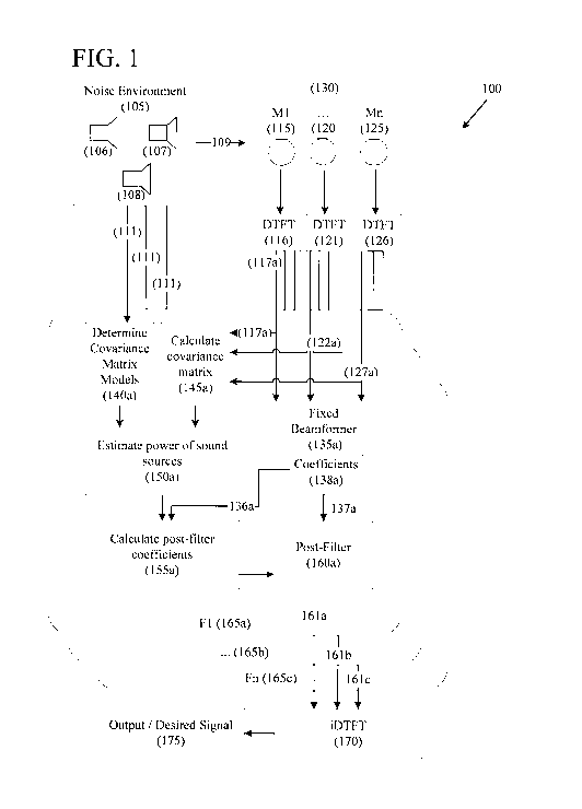
[0008] FIG. 1 is a functional block diagram illustrating an example system
for generating a
post-filtered output signal based on a hypothesized sound field scenario in
accordance with one
or more embodiments described herein.
[0009] FIG. 2 is a functional block diagram illustrating a beamformed
single-channel
output generated from a noise environment in an example system.
[0010] FIG. 3 is a functional block diagram illustrating the determination
of covariance
matrix models based on a hypothesized sound field scenario in an example
system.
CA 3005463 2019-06-28
CA 03005483 2018-05-15
4a
100111 FIG. 4 is a functional block diagram illustrating the post-filter
estimation for a
frequency bin.
[0012] FIG. 5 is a flowchart illustrating example steps for calculating the
post-filter
coefficients for a frequency bin, in accordance with an embodiment of this
disclosure.
100131 FIG. 6 illustrates the spatial arrangement of the microphone array
and the sound
sources related to the experimental results.
100141 FIG. 7 is a block diagram illustrating an exemplary computing
device.
[0015] The headings provided herein are for convenience only and do not
necessarily affect
the scope of the disclosure.
DETAILED DESCRIPTION
[0016] The present disclosure generally relates to systems and methods for
audio signal
processing. More specifically, aspects of the present disclosure relate to
post-filtering techniques
for microphone array speech enhancement.
[0017] The following description provides specific details for a thorough
understanding and
enabling description of the disclosure. One skilled in the relevant art will
understand, however,
that the embodiments described herein may be practiced without many of these
details.
Likewise, one skilled in the relevant art will also understand that the
example embodiments
described herein can include many other obvious features not described in
detail herein.
Additionally, some well-known structures or functions may not be shown or
described in detail
below, so as to avoid unnecessarily obscuring the relevant description.
[0018] 1. Introduction
100191 Certain embodiments and features of the present disclosure relate to
methods and
systems for post-filtering audio signals that utilizes a signal model that
accounts for not only
diffuse and white noise, but also point interfering sources. As will he
described in greater detail
below, the methods and systems are designed to achieve a globally optimized
least-squares (LS)
solution of microphones in a microphone array. In certain implementations, the
performance of
the disclosed method is evaluated using real recorded impulse responses for
the desired and
CA 03005483 2018-05-15
4b
interfering sources, including synthesized diffuse and white noise. The
impulse response is the
output or reaction of a dynamic system to a brief input signal called an
impulse.
100201 FIG. 1
illustrates an example system for generating a post-filtered output signal
(175)
based on a hypothesized sound field scenario (111). A hypothesized sound field
scenario (111) is
a determination of the makeup of the noise components (106-108) in a noise
environment (105).
In practice, when a precise knowledge of the actual sound field composition is
inaccessible,
several different hypotheses about the possible composition can be made. Each
of these
hypotheses are then processed independently, and the best results are output.
According to this
strategy, each hypothesized sound field composition can be called a
hypothesized sound field
scenario. According to systems and methods disclosed herein, a
CA 03005463 2018-05-15
WO 2017/136532 PCT/US2017/016187
plurality of composite scenarios is used, each composite scenario being
composed from sets
of scenarios that are physical locations and/or physical types for each of the
sound sources,
where one composite scenario is selected based on maximizing an objective
function over the
set of scenarios for the desired sound source and minimizing said objective
function over the
set of scenarios for at least one of the interfering sound sources. As a
result, this disclosed
approach can be seen as a more generalized form of other multi-scenario
approaches. In this
example embodiment, one hypothesized sound field scenario (111) is inputted
into the
various frequency bins Fl to Fn (165a-c) to generate an output/desired signal
(175). For a
hypothesized sound field scenario (111), signals are transformed to a
frequency domain.
Beamforming and post-filtering are carried out independently from frequency to
frequency.
[0021] In this example embodiment, a hypothesized sound field scenario
includes one
interfering source. In other example embodiments, hypothesized sound field
scenarios may
be more complex, including numerous interfering scenarios. In other example
embodiments,
where there is no interfering sound source but only diffuse noise in addition
to the desired
sound source, a simpler hypothesized sound field scenario may be used. In
other cases where
there are a plurality of interfering sound sources, a more complicated
hypothesized sound
field scenario with a higher number of acoustic components is used.
[0022] Also, in other example embodiments, multiple hypothesized sound
field scenarios
may be determined to generate multiple output signals. One skilled in the
relevant art will
understand that multiple sound field scenarios may be hypothesized based on
various factors,
such as information that may be known or determined about the environment. One
skilled in
the art will also understand that the quality of the output signals may be
determined using
various factors, such as measuring the signal-to-noise ratio (as measured, for
example, in the
experiments discussed below). In other example embodiments, a person skilled
in the art may
apply other methods to hypothesize sound field scenarios and determine the
quality of the
output signals.
[0023] FIG. 1 illustrates a noise environment (105) which may include one
or more noise
components (106-108). The noise components (106-108) in an environment (105)
may
include, for example, diffuse noise, white noise, and/or point interfering
noise sources. The
noise components (106-108) or noise sources in an environment (105) may be
positioned in
various locations, projecting noise in various directions, and at various
power/strength levels.
Each noise component (106-108) generates audio signals that may be received by
a plurality
CA 03005463 2018-05-15
WO 2017/136532 PCT/US2017/016187
6
of microphones Ml..Mn (115, 120, 125) in a microphone array (130). The audio
signals that
are generated by the noise components (106-108) in an environment (105) and
received by
each of the microphones (115, 120, 125) in a microphone array (130) are
depicted as 109, a
single arrow, in the example illustration for clarity.
[0024] The microphone array (130) includes a plurality of individual
omnidirectional
microphones (115, 120, 125). This embodiment assumes omnidirectional
microphones. Other
example embodiments may implement other types of microphones which may alter
the
covariance matrix models. The audio signals (109) received by each of the
microphones MI
to Mn (where "n" is an arbitrary integer) (115, 120, 125) may be converted to
the frequency
domain via a transformation method, such as, for example, Discrete-time
Fourier
Transformation (DTFT) (116, 121, 126). Other example transformation methods
may
include, but are not limited to, FFT (Fast Fourier Transformation), or STFT
(Short-time
Fourier Transformation). For simplicity, the output signals generated via each
of the DTFT's
(116, 121, 126) corresponding to one frequency are represented by a single
arrow. For
example, the DTFT audio signal at the first frequency bin, Fl (165a),
generated by audio
received by microphone M1 (115) is represented as a single arrow 117a.
[0025] FIG. 1 also illustrates multiple frequency bins (165a-c), which
contain various
components, and where each frequency bin's post-filter component generates a
post-filter
output signal. For instance, frequency bin F1's (165a) post-filter component
(160a) generates
a post-filter output signal of the first frequency bin (161a). The output
signals for each
frequency bin (165a-c) are inputted into an inverse DTFT component (170) to
generate the
final time-domain output! desired signal (175) with reduced unwanted noise.
The details and
steps of the various components in the frequency bins (165a-c) in this example
system (100)
are described in further detail below.
[0026] 2. Signal Models
[0027] FIG. 2 illustrates a beamformed single-channel output (136a)
generated from a
noise environment (105). Components from the overall system 100 (as depicted
in FIG. 1)
not discussed here, have been omitted from FIG. 2 for simplicity. A noise
environment (105)
contains various noise components (106-108) that generate output as sound. In
this example
embodiment, noise component 106 outputs desired sound, and noise components
107 and 108
output undesired sound, which may be in the form of white noise, diffuse
noise, or point
interfering noise. Each of the noise components (106-108) generates sound;
however, for
CA 03005463 2018-05-15
WO 2017/136532 PCT/US2017/016187
7
simplicity, the combined output of the noise components (106-108) is depicted
as a single
arrow 109. The microphones (115, 120, 125) in the array (130) receive the
environment noise
(109) at various time intervals based on the microphone's physical locations
and the
directions and strength of of the incoming audio signals within the
environment noise (109).
The received audio signals at each of the microphones (115, 120, 125) is
transformed (116,
121, 126) and beamformed (135a) to generate a single-channel output (137a) for
one single
frequency. The fixed beamfoimer's (135a) single channel-output (137a) is
passed to the post-
filter (160a). The beamforming coefficients (138a), represented as h(jco),
associated with
Equation (6) below, are generating the beamforming filters (136a) are passed
to calculate
post-filter coefficients (155a).
[0028] A more
detailed description of capturing the environment noise (109) and
generating the beamformed single-channel output signal (137a) and the
beamforming filters
(136a) are described here. Suppose a microphone array (130) ofM elements (115,
120, 125),
where M, an arbitrary integer value, is the number of microphones in the array
(130), to
capture the signal s(t) from a desired point sound source (106) in a noisy
acoustic
environment (105). The output of the mth microphone in the time domain is
written as
(.0 -------- 9%45,k,.= * (t) + 114VA M = 1,2, - M,
0)
where gs,m denotes the impulse response from the desired component (106) to
the mth
microphone (e.g. 125), * denotes linear convolution, and vm(t) is the unwanted
additive noise
(i.e., sound generated by noise components 107 and 108).
The disclosed method is capable of dealing with multiple point interfering
sources;
however, for clarity, one point interferer is described in the examples
provided herein. The
additive noise commonly consists of three different types of sound components:
1) coherent
noise from a point interfering source, v(t), 2) diffuse noise, um(t), and 3)
white noise, w(t).
Also,
+ um (.0 + 1.1h4 (2)
where gvm, is the impulse response from the point noise source to the mth
microphone. In this
example embodiment, the desired signal and these noise components (106-108)
are presumed
short-time stationary and mutually uncorrelated. In other example embodiments,
the noise
CA 03005463 2018-05-15
WO 2017/136532 PCT/US2017/016187
8
components may be comprised differently. For example, a noise environment
which contains
multiple desired sound sources moving around and the target desired sound
source may
alternate over a time period. In other words, a crowded room where two people
are walking
while having a conversation.
[0029] In the
frequency domain, this generalized microphone array signal model in
Equation (1) is transformed into
jw) = C õ,õ(jw)S (iw) + ( jw)
= ,õõ,(it-a)s jw)V (i6o)
(,M W(jw) (3)
A , 7
where =V, co
is the angular frequency, and Xm(jco), G,,,õ(jco), S(jc0), Gv,15(10)), V
(lco),
U(Ico), W(Ico) are the discrete-time Fourier transforms (DTFTs) of xni(t),
gs,m, s(t), gym, v(t),
u(t), and w(t), respectively. In the example embodiments, DTFT is implemented;
however, it
should not be construed to limit the scope of the invention. Other example
embodiments may
implement other methods such as STFT (Short Time Fourier Transformation) or
FFT (Fast
Fourier Transformation). Equation (3) in a vector/matrix form is as follows
x(j) = S(jai)1,4(jw) + (jlt,")gw) + u(j) + w*), (4)
where
zUw) .................. I 71(j4:4)) Zgjut) - 2 Cit.41) fr) ZE w},
= 1T
(jw) (jw) G.,2(iw) = = = C4,..kiCke) ) Z E
OT denotes the transpose of a vector or a matrix The microphone array spatial
covariance
matrix is then determined as
Ra-x(jw) ................. crRw)P& (jw) + (5)
, , ,
= fa) cy,¨Ptv, Uth) RIV'W(iµv),
where mutually uncorrelated signals are assumed,
R E
if = , = õ (jw). .. =
jw) ................................ (jlw)&11: "(it.e), z E ts,
E [7(p) (jw)} E {s, v},
CA 03005463 2018-05-15
WO 2017/136532 PCT/US2017/016187
9
and Ell, Off, and (=)* denote the mathematical expectation, the Hermitian
transpose of a
vector or matrix, and the conjugate of a complex variable, respectively.
[0030] A beamformer (135a) filters each microphone signal by a finite
impulse response
(FIR) filter 1-1,7(jco) (m = 1, 2, = = = , Al) and sums the results to produce
a single-channel
output (137a)
E h.fr(iw.)x(iz,), (0)
In= I
and beamfol tiling filters (136a), where
-T
hUw) ................................. [ 1:11(jce) 112:Ute). n Ilm (ILO
[0031] In Equation (6), the covariance matrix of the desired sound source
is also
modeled. Its model is similar to that of the interfering source since both the
desired and the
interfering sources are point source. They differ in their directions with
respect to the
microphone array.
CA 03005463 2018-05-15
WO 2017/136532 PCT/US2017/016187
[0032] 3. Modeling Noise Covariance Matrices
[0033] FIG. 3 illustrates the steps for determining covariance matrix
models based on a
hypothesized sound field scenario (111). Components from the overall system
100 (as
depicted in FIG. 1) not discussed here, have been omitted from FIG. 3 for
simplicity. A
hypothesized sound field scenario (111) is determined based on the makeup of
the noise
components (106-108) in the noise environment (105) and inputted into the
covariance
models (140a-c) for each frequency bin (165a-c) respectively.
[0034] In an actual environment, the makeup of noise components, i.e. the
number and
location of point interfering sources and the presence of white or diffuse
noise sources may
not be known. Thus, a sound field scenario is hypothesized. Equation (2) above
represents a
scenario with one point interfering source, diffuse noise, and white noise,
resulting in four
unknowns. If the scenario hypothesizes or assumes no point interfering source,
only white
and diffuse noise, the above Equation (5) can then be simplified resulting in
only three
unknowns.
[0035] In Equation (5), three interference/noise-related components (106-
108) are
modeled as follows:
[0036] (1) Point Interferer: The covariance matrix Pg,, (jco) due to the
point interfering
source v(t) has rank 1. In general, when reverberation is present or the
source is in the near
field of the microphone array, the complex elements of the impulse response
vector gv may
have different magnitudes. But if only the direct path is taken into account
or if the point
source is in the far field, then
gv ow) = m
which incorporates only the interferer's time differences of arrival at the
multiple
microphones r (m = 1, 2, = = = , M) with respect to a common reference point.
[0037] (2) Diffuse Noise: A diffuse noise field is considered spherically
or cylindrically
isotropic, in that it is characterized by uncorrelated noise signals of equal
power propagating
in multiple directions simultaneously. Its covariance matrix is given by
Rictg (i.W) '' Crtl ("))1:'11.4 (sW).'
where the (p, q)th element of r(w) is
CA 03005463 2018-05-15
WO 2017/136532 PCT/US2017/016187
11
SineI _________________________________ dPg Spherically hawk
. c
= I(9)
= psq
[ ____________________________________________________________ .,µ
Cylindtically Isotropic
dpq is the distance between the pth and gth microphones, c is the speed of
sound, and J0(.) is
the zero-order Bessel function of the first kind.
[0038] (3) White Noise: The covariance matrix of additive white noise is
simply a
weighted identity matrix:
= x (10)
[0039] 4. Multichannel Wiener Filter (MCWF), MVDR Beamforming, and Post-
Filtering
[0040] When a microphone array is used to capture a desired wideband sound
signal
(e.g., speech and/or music), the intention is to minimize the distance between
Y (jco) in
Equation (6) and S(Jco) for co's. The MCWF that is optimal in the MMSE sense
can be
decomposed into a MVDR beamformer followed by a single-channel Wiener filter
(SCWF):
R;11; (*)14.ji. w
hmcwc(ita) ........................................................ , (1 I.)
gl:,1 (JO 931e) g7õ2t (zA") (w)
''....yeinsmommmomPf
464VDR (2`.0 A htstvp(tO,
where
(th) .t.r! (i.e) htivDR(jf.e) .( jw)hmvim.
(a.,) hffvDri (iw )Roo (i0hmvniz. Ow)
are the power of the desired signal and noise at the output of the MVDR
beamformer,
respectively. This decomposition leads to the following stnicture for
microphone array
speech acquisition: the SCWF is regarded as a post-filter after the MVDR
beamformer.
[0041] 5. Post-Filter Estimation
[0042] FIG. 4 illustrates the post-filter estimation steps in a frequency
bin. In order to
implement the front-end MVDR beamformer and the SCWF as a post-processor given
in
Equation (11), the signal and noise covariance matrices from the calculated
covariance matrix
of the microphone signals are estimated. The multichannel microphone signals
are first
windowed (e.g., by a weighted overlap-add analysis window) in frames and then
transformed
by a FFT to determine x(jco, i), where i is the frame index. The estimate of
the microphone
CA 03005463 2018-05-15
WO 2017/136532 PCT/US2017/016187
12
signals' covariance matrix (145a) is recursively updated, dynamically or using
a memory
component, by
.IL(jw7i):az (jai, (1.
i)xn(jwi), (12)
where 0 < A < 1 is a forgetting factor.
[0043] Again, similar to Equation (7), reverberation may be ignored,
resulting in
[ õ yit (13)
where r,,, is the desired signal's time difference of arrival for the mth
microphone with
respect to the common reference point.
[0044] In another example, suppose that both Ts,õ, and T
- v, are known and do not change
over time. Thus, according to Equation (5), using Equation (8) and Equation
(10), at the ith
time frame, the determination of the covariance matrix models (140a) may be
determined as
follows:
itõ.õ(jw, i) =t7,2_ (w, ) u.", i)Pgv(jW)
I48 (5)J act ((e.. -01.A4 (14)
This equality allows defining a criterion based on the Frobenius norm of the
difference
between the left and the right hand sides of Equation (14) By minimizing such
a criterion, an
LS estimator for {o-2 (co, k), o-2 (co, k), o-2 (co, k), o-2 (co, k)} may be
deduced Note that the
s v w
matrices in Equation (14) are Hermitian Redundant information in this
formulation has been
omitted for clarity.
[0045] For an M
x M Hermitian matrix A = [apq], two vectors may be defined. One
vector is the diagonal elements and the other is the off-diagonal half
vectorization (odhv) of
its lower triangular part
diagtA =[ an at22 = = am m (15)
Why [1121 " = am am = " am 2 = = am of ... - 06)
A plurality of NHermitian matrices of the same size may be defined as
diag {A diagiAll = = di
agtA. N1 .. 07)
odlxv { At, ¨ AN). godiavl ALI - odhv {AN } (18)
By using these notations, Equation (14) is reorganized to get
CA 03005463 2018-05-15
WO 2017/136532 PCT/US2017/016187
13
= (4 ' X(k)f (19)
where parameter jco is omitted for clarity, and
dhe R Ow k)} . A - lkiik,f ) -
Why { it- õõ ( jw:, k) I _ ' 8' C(ial) '
DC*) --4. din Mg, (ILO, .P.õ (jC4)), F.,,,:.(jw), IA.i.x.m I,
C(ico) =--1.'. edhv t Pgt,:(j-w), P (jw), r,,,..(jw), "Mx m 1 ,
[ 41.! (wt. k) a.(.to k) cr:!(.= k)
Here, the result is M (M + 1) / 2 equations and 4 unknowns. If M > 3, this is
an
overdetermined problem. That is, there are more equations than unknowns.
[0046] The aforementioned error criterion is written as
3 2
j A I iltjk) ¨ 0 - xtk)11 (20)
Minimizing this criterion, implemented as estimating the power of sound
sources (150a),
leads to
*Is (k): = it (elle) ¨1. F10.144 (k) {
(21.)
where n / denotes the real part of a complex number/vector. Presumably the
estimation
,
0 (k)
errors in afm' , are IID (independent and identically distributed) random
variables. Thus, as
implemented in calculating the post-filter coefficients (155a), the LS (least-
squares) solution
given in Equation (21) is optimal in the MMSE sense. Substituting this
estimate into
Equation (11) leads to, as referred to in this disclosure, a LS post-filter
(LSPF) (160a).
[0047] In the
above described example embodiment, the deduced LS solution assumes
that M> 3. This is due to the use of a more generalized acoustic-field model
that consists of
four types of sound signals. In other example embodiments, where additional
information
regarding the acoustic field is available, such that some types of interfering
signals can be
ignored (e g , no point interferer and/or merely white noise), then those
columns in Equation
(19) that correspond to these ignorable sound sources can be removed and an
LSPF as
described in the present disclosure may still be developed even with M= 2.
[0048] FIG. 5
is a flowchart illustrating example steps for calculating the post-filter
coefficients for a frequency bin (165a), in accordance with an embodiment of
this disclosure.
CA 03005463 2018-05-15
WO 2017/136532 PCT/US2017/016187
14
The following illustration in FIG. 5 reflects an example implementation of the
above
disclosed details and mathematical concepts described above. The disclosed
steps are given
by way of illustration only. As would be apparent to one skilled in the art,
some steps may be
done in parallel or in an alternate sequence within the spirit and scope of
this Detailed
Description.
[0049] Referring to FIG. 5, the example steps start at step 501. In step
502, audio signals
are received via microphone array (130) from noise generated (109) by sound
sources (106-
108) in an environment (105). In step 503, a sound field scenario (111) is
hypothesized. In
step 504, fixed beamformer coefficients (138a) are calculated based on the
received audio
signals (117a, 122a, 127a) for a frequency bin (165a). In step 505, covariance
matrix models
(140a) based on the hypothesized sound field scenario (111) are determined. In
step 506, a
covariance matrix (145a) based on the received audio signals (117a, 122a,
127a) is
calculated. In step 507, the power of the sound sources (150a), based on the
determined
covariance matrix models (140a) and the calculated covariance matrix (145a),
are estimated.
In step 508, post-filter coefficients (155a), based on the estimated power of
the sound sources
(150a) and the calculated fixed beamformer coefficients (138a), are
calculated. The example
steps may proceed to the end step 509. The aforementioned steps may be
implemented per
frequency bin (165a-c) to generate the post-filtered output signals (161a-c)
respectively. The
post-filtered signals (161a-c) may then be transformed (170) to generate the
final
output/desired signal (175).
[0050] As mentioned above, conventional post-filtering methods are not
optimal and
have deficiencies when compared to methods and systems described herein. The
limitations
and deficiencies of existing approaches, with respect to the present
disclosure, are further
described below.
2
[0051] (a) Zelinski's Post-Filter (ZPF) assumes: 1) no point interferer,
i.e., o-V (co) = 0,
2
2), no diffuse noise, i.e., au (w) = 0, and 3) only additive incoherent white
noise. Thus,
Equation (19) is simplified as follows
diag tt - ding{ P1,4 x cr:i(k)'
odhv (It% õ (k) Why {1%, 0 - 01(k)
CA 03005463 2018-05-15
WO 2017/136532 PCT/US2017/016187
2
Instead of calculating the optimal LS solution for as (k) using Equation (21),
the ZPF uses
only the bottom odhv-part of Equation (22) to get
{o&/v{tt.- (k)}}
La v=1
ti 0 Ast: vi..1 = O ¨1)2 .. 1-1 (23)
\--cm w / R foithv A., }Iv
Note, from Equation (13) that R {odhv (Pgs} }p = 1. Thus, Equation (23)
becomes
--, ,,,.,..i. = = N i dire fit%,õ(k)).11.
624721-0) ¨ . P , (24)
If the same acoustic model for the LSPF is used for ZPF (e.g., only white
noise), it can be
shown that the ZPF and the LSPF are equivalent when M= 2. However, they are
fundamentally different when M? 3.
2
[0052] (b)
McCowan's Post-Filter (MPF) assumes: 1) no point interferer, i e , o-v (co) =
9
0, 2), no additive white noise, i.e., o-w (co) = 0, and 3) only diffuse noise.
Under these
assumptions, Equation (19) becomes
- diag{ii,,,,,, (k)}- - dial! { P } diag {F } - 0-2 1 0,5 k)
õ...
' k = t"6- ; N .. )
ptillvtR.,,,(k)1_ _0(1hv {Pg8 } dim fr.o [ _ a-,,,; (k)
Note from Equation (9) that diag {rõ} = 1 Afx 1.
[0053] Equation
(25) is an overdetermined system. Again, instead of finding a global LS
solution by following Equation (21), the MPF applies three equations from
Equation (25) that
correspond to the pair of the pth and qth microphones to form a subsystem like
the following
07-.2
[ _
1 I - 2 -
(3'2 ¨ 1 I
0:1,13 'IV .,.:1 rp=
q
where
Ppq 111 ai { Fts Ti. } p,v
2
The MPF method solves Equation (26) for o-, as
CA 03005463 2018-05-15
WO 2017/136532 PCT/US2017/016187
16
=poi
";;q (Porog,
1,07*,MPF}p,4 ______________________________________________________ = (27)
¨ rpfg
Since there are Al (M ¨ 1)/ 2 different microphone pairs, the final MPF
estimate is simply
the average of the subsystems' results, as follows:
1µ.. 2 24.-4s=1.
L...eq=p4-11.1s e3 MPIlp.q
ua,N11-17
M (111- -- 1)/2
[0054] The diffuse noise model is more common in practice than the white
noise model.
The latter can be regarded as a special case of the former when Tuõ = I1xM.
But the MPF's
approach to solving Equation (25) is heuristic and is also not optimal. Again,
if LSPF uses a
diffuse-noise-only model, it is equivalent to the MPF when M = 2, but they are
fundamentally
different when Al> 3.
[0055] (c) Leukimmiatis's Post-Filter follows the algorithm proposed in the
MPF to
2
estimate us (k). Leukimmiatis et al. simply fixes the bug in Zelinski's and
McCowan's
2 2
postfilters that the denominator of the post-filter in (11) should be o-st
(co) + o- III (co) rather
2
than o-s (co) + o- (co).
CA 03005463 2018-05-15
WO 2017/136532 PCT/US2017/016187
17
[0056] 6. Experimental Results
[0057] The following provides results of example speech enhancement
experiments
performed to validate the LSPF method and systems of the present disclosure.
FIG. 6
illustrates the spatial arrangement of the microphone array (610) and the
sound sources (620,
630) of the experiments. The positions of the elements within the figures are
not intended to
convey exact scale or distance, which are provided in the following
description. Provided are
a set of experiments that consider the first four microphones Ml-M4 (601-604)
of a
microphone array (610), where the spacing between each of the microphones is 3
cm. The 60
dB reverberation time is 360 ms. The desired source (620) is at the broadside
(0 ) of the array
while the interfering source (630) is at the 45. direction. Both are 2m from
the array. Clean,
continuous, 16 kHz/16-bit speech signals are used for these point sound
sources. The desired
source (620) is a female speaker and the interfering source (630) is a male
speaker. The
voiced parts of the two signals have many overlaps. Accordingly, the impulse
responses are
resampled at 16 kHz and are truncated to 4096 samples and spherically
isotropic diffuse noise
is generated. In the experimental simulations, 72 x 36 = 2592 point sources
distributed on a
large sphere are used. The signals are truncated to 20 s.
[0058] In the above experiments, three full-band measures are defined to
characterize a
sound field (subscript SF): namely, the signal-to-interference ratio (SIR),
signal-to-noise ratio
(SNR), and diffuse-to-white-noise ratio (DWR), as follows
STR.sF 10 = logIcAt7Lify,2,1, (29)
SNRatõ 10 = log mfp!Acii! (30)
DWR&F :10 log ,510-õ2/0-1 (31)
wherecf2õ: Elziltll and z E fa. v LAO-
-
[0059] For performance evaluation, two objective metrics are analyzed: the
signal-to-
interference-and-noise ratio (SINR) and the perceptual evaluation speech
quality (PESQ).
The SINR' s and PESQ's are computed at each microphone and averaged as the
input SINR
and PESQ, respectively. The output SINR and PESQ (denoted by SINRo and PESQo,
respectively) are similarly estimated. The difference between the input and
output measures
(i.e., the delta values) are analyzed. To better assess the amount of noise
reduction and speech
distortion at the output, the interference and noise reduction (INR) and the
desired-speech
only PESQ (dPESQ) are also calculated. For dPESQ's, the processed desired
speech and
clean speech is passed to the PESQ estimator. The output PESQ indicates the
quality of the
CA 03005463 2018-05-15
WO 2017/136532 PCT/US2017/016187
18
enhanced signal while the dPESQ value quantifies the amount of speech
distortion
introduced. The Hu & Loizou's Matlab codes for PESQ are used in this study.
[0060] To avoid the well-known signal cancellation problem in the MVDR
(minimum
variance distortionless response) beamformer due to room reverberation, the
delay-and-sum
(D&S) beamformer is implemented for front-end processing and compared to the
following
four different post-filtering algorithms: none, ZPF, MPF, and LSPF. The D&S-
only
implementation is used as a benchmark. For ZPF and MPF, Leukimmiatis's
correction has
been employed. Tests were conducted under the following three different
setups: 1) White
Noise ONLY: SIRSF = 30 dB, SNRSF = 5 dB, DWRSF = ¨30 dB, 2) Diffuse Noise
ONLY:
SIRSF = 30 dB, SNRSF = 10 dB, DWRSF = 30 dB, 3) Mixed Noise/Interferer: SIRSF
= 0
dB, SNRSF = 10 dB, DWRSF = 0 dB. The results are as follows:
Table 1: Microphone array speech enhancement results.
Method .1NR SINR, / PESOõ. / dPESQ, .1
(dR) A.S1.NR (dB) LPESQ AdPESQ
White Noise Only
.D&S Only 5.978 14.2W/ +5..6$ 1.79540363 2.286/4.019
.D&S+ZPF 11193 .17.827/+9.293 2,05540.623 235140.046
:D&S+MPF 16.924 17.1611 +8.627 2.1151+0.683 2.1301-0.175
1186+1..SPF 11858 21.460412.925 218040.748 2.2991Ø006
Diffuse Noise Only'
:D&S Only 3.7.35 16.9.151 +3.423 1.8521+0.088 2,2861-0.019
D&S+ZPF 7.467 18.5941+5.102 1.95440.1.90 231140.006
.D&S+MPF 111012 16.545/ +3..053 2.12240358 2.42740,1:21
D&S+LS.PF .12,236 17.699/ +4107 125440..490 151640,211
Mixed NoiNclInteilltre4-
:D&S Only 0,782 23981 +0.435 1.49340.122 2.28614019
D&S+ZPF 2.879 2.424/+0.461 1.56340.193 2.31440.009
D&S+MPF 9.470 4.211/+2.248 1.79140.420 2.297/-0.008
:D&S+LSPF 16374 9173/ +7..810 1.94040.569 233640.031
[0061]
[0062] In these tests, the square-root Hamming window and 512-point FFT are
used for
the STFT analysis. Two neighboring windows have 50% overlapped samples. The
weighted
overlap-add method is used to reconstruct the processed signal.
[0063] The experimental results are summarized in Table 1. First, the
results for the
white-noise-only sound field are analyzed. Since this is the type of sound
field addressed by
CA 03005463 2018-05-15
WO 2017/136532 PCT/US2017/016187
19
the ZPF method, the ZPF does a reasonably good job in suppressing noise and
enhancing
speech quality. However, the proposed LSPF achieves more noise reduction and
offers higher
output PESQ, albeit it introduces more speech distortion with a slightly lower
dPESQ. The
MPF produces a deceptively high INR since its SINR gain is lower than that of
the ZPF and
LSPF. This means that the MPF significantly suppresses not only noise but also
speech
signals. Its PESQ and dPESQ are lower than that of the LSPF.
[0064] In the second sound field, as expected that the D&S beamformer is
less effective
to deal with diffuse noise and the ZPF's perfoitnance degrades too. In this
case the MPF's
performance is reasonably good while still the LSPF yields evidently best
results.
[0065] The third sound field is apparently the most challenging case to
tackle due to the
presence of a time-varying interfering speech source. However, the LSPF
outperforms the
other conventional methods in all metrics.
[0066] Finally, it is noteworthy that these purely objective performance
evaluation results
are consistent with subjective perception of the four techniques in informal
listening tests
carried out with a small number of our colleagues.
[0067] The present disclosure describes methods and systems for a LS post-
filtering
method for microphone array applications. Unlike conventional post-filtering
techniques, the
method described considers not only diffuse and white noise but also point
interferers.
Moreover it is a globally optimal solution that exploits the information
collected by a
microphone array more efficiently than conventional methods. Furthermore, the
advantages
of the disclosed technique over existing methods has been validated and
quantified by
simulations in various acoustic scenarios.
[0068] FIG. 7 is a high-level block diagram to show an application on a
computing
device (700). In a basic configuration (701), the computing device (700)
typically includes
one or more processors (710), system memory (720), and a memory bus (730). The
memory
bus is used to do communication between processors and system memory. The
configuration
may also include a standalone post-filtering component (726) which implements
the method
described above, or may be integrated into an application (722, 723).
[0069] Depending on different configurations, the processor (710) can be a
microprocessor ([113), a microcontroller (p.C), a digital signal processor
(DSP), or any
combination thereof The processor (710) can include one or more levels of
caching, such as
a Li cache (711) and a L2 cache (712), a processor core (713), and registers
(714). The
CA 03005463 2018-05-15
WO 2017/136532 PCT/US2017/016187
processor core (713) can include an arithmetic logic unit (ALU), a floating
point unit (FPU),
a digital signal processing core (DSP Core), or any combination thereof. A
memory
controller (716) can either be an independent part or an internal part of the
processor (710).
[0070] Depending on the desired configuration, the system memory (720) can
be of any
type including but not limited to volatile memory (such as RAM), non-volatile
memory (such
as ROM, flash memory, etc.) or any combination thereof. System memory (720)
typically
includes an operating system (721), one or more applications (722), and
program data (724).
The application (722) may include a post-filtering component (726) or a system
and method
to apply globally optimized least-squares post-filtering (723) for speech
enhancement.
Program Data (724) includes storing instructions that, when executed by the
one or more
processing devices, implement a system and method for the described method and
component. (723). Or instructions and implementation of the method may be
executed via
post-filtering component (726). In some embodiments, the application (722) can
be arranged
to operate with program data (724) on an operating system (721).
[0071] The computing device (700) can have additional features or
functionality, and
additional interfaces to facilitate communications between the basic
configuration (701) and
any required devices and interfaces.
[0072] System memory (720) is an example of computer storage media.
Computer
storage media includes, but is not limited to, RAM, ROM, EEPROM, flash memory
or other
memory technology, CD-ROM, digital versatile disks (DVD) or other optical
storage,
magnetic cassettes, magnetic tape, magnetic disk storage or other magnetic
storage devices,
or any other medium which can be used to store the desired information and
which can be
accessed by computing device 700. Any such computer storage media can be part
of the
device (700).
[0073] The computing device (700) can be implemented as a portion of a
small-form
factor portable (or mobile) electronic device such as a cell phone, a smart
phone, a personal
data assistant (PDA), a personal media player device, a tablet computer
(tablet), a wireless
web-watch device, a personal headset device, an application-specific device,
or a hybrid
device that includes any of the above functions. The computing device (700)
can also be
implemented as a personal computer including both laptop computer and non-
laptop
computer configurations.
CA 03005463 2018-05-15
21
[00741 The foregoing detailed description has set forth various embodiments
of the devices
and/or processes via the use of block diagrams, flowcharts, and/or examples.
Insofar as such
block diagrams, flowcharts, and/or examples contain one or more functions
and/or operations, it
will be understood by those within the art that each function and/or operation
within such block
diagrams, flowcharts, or examples can be implemented, individually and/or
collectively, by a
wide range of hardware, software, firmware, or virtually any combination
thereof. In one
embodiment, several portions of the subject matter described herein may be
implemented via
Application Specific Integrated Circuits (ASICs), Field Programmable Gate
Arrays (FPGAs),
digital signal processors (DSPs), or other integrated formats. However, those
skilled in the art
will recognize that some aspects of the embodiments disclosed herein, in whole
or in part, can be
equivalently implemented in integrated circuits, as one or more computer
programs running on
one or more computers, as one or more programs running on one or more
processors, as
firmware, or as virtually any combination thereof, and that designing the
circuitry and/or writing
the code for the software and/or firmware would be well within the skill of
one skilled in the art
in light of this disclosure. In addition, those skilled in the art will
appreciate that the mechanisms
of the subject matter described herein are capable of being distributed as a
program product in a
variety of forms, and that an illustrative embodiment of the subject matter
described herein
applies regardless of the particular type of non-transitory signal bearing
medium used to actually
carry out the distribution. Examples of a non-transitory signal bearing medium
include, but are
not limited to, the following: a recordable type medium such as a floppy disk,
a hard disk drive, a
Compact Disc (CD), a Digital Video Disk (DVD), a digital tape, a computer
memory, etc.; and a
transmission type medium such as a digital and/or an analog communication
medium. (e.g., a
fiber optic cable, a waveguide, a wired communications link, a wireless
communication link,
etc.)
100751 With respect to the use of any plural and/or singular terms herein,
those having skill
in the art can translate from the plural to the singular and/or from the
singular to the plural as is
appropriate to the context and/or application. The various singular/plural
permutations may be
expressly set forth herein for sake of clarity.
CA 03005463 2018-05-15
21a
100761 Thus, particular
embodiments of the subject matter have been described. Other
embodiments are within the scope of the disclosure. In some cases, the actions
recited in the
disclosure can be performed in a different order and still achieve desirable
results. In
CA 03005463 2018-05-15
WO 2017/136532 PCT/US2017/016187
22
addition, the processes depicted in the accompanying figures do not
necessarily require the
particular order shown, or sequential order, to achieve desirable results. In
certain
implementations, multitasking and parallel processing may be advantageous.
[0077] In the following, further examples of the system and method
according to the
present disclosure are described.
[0078] A first example of a computer-implemented method comprises receiving
audio
signals via a microphone array from sound sources in an environment,
hypothesizing a sound
field scenario based on the received audio signals, calculating fixed
beamformer coefficients
based on the received audio signals, determining covariance matrix models
based on the
hypothesized sound field scenario, calculating a covariance matrix based on
the received
audio signals, estimating power of the sound sources to find solution that
minimizes the
difference between the determined covariance matrix models and the calculated
covariance
matrix, calculating and applying post-filter coefficients based on the
estimated power, and
generating an output audio signal based on the received audio signals and the
post-filter
coefficients.
[0079] A second example: the method of the first example, further
comprising
hypothesizing multiple sound field scenarios to generate multiple output
signals.
[0080] A third example: the method of the second example, wherein the
multiple
generated output signals are compared and the output signal with the highest
signal-to-noise
ratio among the multiple output generated signals is selected as the final
output signal
[0081] A fourth example: the method of one of examples one to three,
wherein the
estimating of the power is based on the Frobenius norm.
[0082] A fifth example: The method of one of examples one to four, wherein
the
Frobenius norm is computed using the Hermitian symmetry of the covariance
matrices.
[0083] A sixth example: The method of one of examples one to five, further
comprising:
determining the location of at least one of the sound sources using sound-
source location
methods to hypothesize the sound field scenario, determine the covariance
matrix models,
and calculate the covariance matrix.
[0084] A seventh example: The method of one of examples one to six, wherein
the
covariance matrix models are generated based on a plurality of hypothesized
sound field
scenarios.
CA 03005463 2018-05-15
WO 2017/136532 PCT/US2017/016187
23
[0085] An eighth example: The method of example seven, wherein a covariance
matrix
model is selected to maximize an objective function that reduces noise.
[0086] A ninth example: The method of example eight, wherein an objective
function is
the sample variance of the final output audio signal.
[0087] A tenth example: an apparatus, comprising one or more processing
devices and
one or more storage devices storing instructions that, when executed by the
one or more
processing devices, cause the one or processing devices to: receive audio
signals via a
microphone array from sound sources in an environment, hypothesize a sound
field scenario
based on the received audio signals, calculate fixed beamformer coefficients
based on the
received audio signals, determine covariance matrix models based on the
hypothesized sound
field scenario, calculate a covariance matrix based on the received audio
signals, estimate
power of the sound sources to find solution that minimizes the difference
between the
determined covariance matrix models and the calculated covariance matrix,
calculate and
applying post-filter coefficients based on the estimated power, and generate
an output audio
signal based on the received audio signals and the post-filter coefficients.
[0088] An eleventh example: the apparatus of example ten, further
comprising of
hypothesizing multiple sound field scenarios to generate multiple output
signals.
[0089] A twelfth example: the apparatus of example eleven, wherein the
multiple
generated output signals are compared and the output signal with the highest
signal-to-noise
ratio among the multiple output generated signals.
[0090] A thirteenth example: the apparatus of one of example ten to twelf,
wherein the
estimating of the power is based on the Frobenius norm.
[0091] A fourteenth example: the apparatus of one of examples ten to
thirteen, wherein
the Frobenius norm is computed using the Hermitian symmetry of the covariance
matrices.
[0092] A fifteenth example: the apparatus of one of examples ten to
fourteen, further
comprising determining the location of at least one of the sound sources using
sound-source
location methods to hypothesize the sound field scenario, determine the
covariance matrix
models, and calculate the covariance matrix.
[0093] A sixteenth example: a computer-readable medium, comprising sets of
instructions for: receiving audio signals via a microphone array from sound
sources in an
environment, hypothesizing a sound field scenario based on the received audio
signals,
calculating fixed beamformer coefficients based on the received audio signals,
determining
CA 03005463 2018-05-15
WO 2017/136532 PCT/US2017/016187
24
covariance matrix models based on hypothesized sound field scenario,
calculating a
covariance matrix based on the received audio signals, estimating power of the
sound sources
to find solution that minimizes the difference between the determined
covariance matrix
models and the calculated covariance matrix, calculating and applying post-
filter coefficients
based on the estimated power, and
generating an output audio signal based on the received audio signals and the
post-filter
coefficients.
[0094] A seventeenth example: the computer-readable medium of example
sixteen,
wherein multiple hypothesized sound field scenarios to generate multiple
output signals.
[0095] An eighteenth example: the computer-readable medium of example
seventeen,
wherein the multiple generated output signals are compared and the output
signal with the
highest signal-to-noise ratio among the multiple output generated signals.
[0096] A nineteenth example: the computer-readable medium of one of
examples sixteen
to eighteen, wherein the estimating of the power is based on the Frobenius
norm.
[0097] A twentieth example: the computer-readable medium of one of examples
sixteen
to nineteen, wherein the Frobenius norm is computed using the Hermitian
symmetry of the
covariance matrices.
[0098] A twenty-first example: the computer program comprising sets of
instructions
which when being executed by a computer carry out the method of one of
examples one to
nine.
[0099] Existing post-filtering methods for microphone array speech
enhancement have
two common deficiencies. First, they assume that noise is either white or
diffuse and cannot
deal with point interferers. Second, they estimate the post-filter
coefficients using only two
microphones at a time, performing averaging over all the microphones pairs,
yielding a
suboptimal solution. According to embodiments described therein, there are
provided
methods describing a post-filtering solution that implements signal models
which handle
white noise, diffuse noise, and point interferers. According to embodiments,
the methods also
implement a globally optimized least-squares approach of microphones in a
microphone
array, providing a more optimal solution than existing conventional methods.
Experimental
results demonstrate the described method outperforming conventional methods in
various
acoustic scenarios.