Note: Descriptions are shown in the official language in which they were submitted.
CA 03005600 2018-05-16
WO 2017/086762
PCT/KR2016/013423
METHOD FOR CALIBRATING A DATA SET OF A TARGET ANALYTE
FIELD OF THE INVENTION
The present invention relates to a method for calibrating a data set of a
target
analyte in a sample.
BACKGROUND OF THE INVENTION
A polymerase chain reaction (hereinafter referred to as "PCR") which is most
widely
io used for
the nucleic acid amplification includes repeated cycles of cldnaturation of
double-
stranded DNA, followed by oligonucleotide primer annealing to the DNA
template, and
primer extention by a DNA polymerase (Mullis et al., U. S. Pat. Nos.
4,683,195, 4,683,202
and 4,800,159; Saiki et al., (1985) Science 230, 1350-1354)
A real-time polymerase chain reaction is one of PCR-based technologies for
detecting
a target nucleic acid molecule in a sample in a real-time manner. For
detecting a specific
target analyte, the real-time PCR uses a signal-generating means for
generating a
fluorescence signal being detectable in a proportional manner with the amount
of the target
molecule. The generation of fluorescence signals may be accomplished by using
either
intercalators generating signals when intercalated between double-stranded DNA
or
oligonucleotides carrying fluorescent reporter and quencher molecules. The
fluorescence
signals whose intensities are proportional with the amount of the target
molecule are
detected at each amplification cycle and plotted against amplification cycles,
thereby
obtaining an amplification curve or amplification profile curve.
A sample analysis using fluorescence signals is performed as follow. When a
luminant
is supplied with energy through a light source such as LED, electron of the
luminant is
excited to a higher quantum state, then the luminant emits a light of specific
wavelength by
relaxation of the orbital electron to its ground state. Analytical instrument
converts the light
of specific wavelength to an electric signal using photodiode or CCD and
provides
information needed for sample analysis. Although the same amount of a luminant
in a
CA 03005600 2018-05-16
WO 2017/086762
PCT/KR2016/013423
sample is analyzed, each analytical instrument provides different signal
values because of
the uneven illuminations of the light source (e.g., LED) and the performance
variations of
the light-electricity conversion device in the respective instruments. Such a
signal difference
between instruments is called as an inter-instrument variation. In addition to
the inter-
s instrument variation, the analysis results of a plurality of reactions
performed for the same
kind and the same amount of the target analyte by a single identical
analytical instrument
may have variations in signal level because of the difference in reaction
environments such
as the position of reaction well where the reaction is performed on the
instrument or
delicate differences in composition or concentration of the reaction mixture.
Such a signal
difference among the reactions in a single instrument is known as an intra-
instrument
variation. Furthermore, an electrical noise signal is generated by an
analytical instrument
itself even when a blank (matrix without analyte) is analyzed and it may be
identified as a
normal signal. However, such an electrical noise signal also creates a signal
variation and is
referred to as an instrument blank signal. The instrument blank signal is
generated in a
Is .. manner that a specific amount of signal value is added to or subtracted
from the original
signal value for each cycle.
For the precise and reliable analysis, such problems have to be solved and
several
methods are used to solve the problems. As a most basic solution, a hardware
adjustment
method is used. For instance, when the analytical instrument is manufactured,
the property
of some parts of each analytical instrument such as intensity of LED light
source is calibrated
or adjusted such that the level of an inter-instrument variation for the same
sample is
reduced and maintained within, a proper range. Alternatively, a reference dye
method may
be used. The reference dye such as ROXIN or fluorescein which constantly
generates a
known amount of a signal is added in a reaction mixture such that the signal
generated from
a sample is calibrated based on the level of signal generated from the
reference dye.
However, these prior art may have some limitations or shortcomings. The
hardware
adjustment method shows limited accuracy in calibration and an additional
calibration is
needed to remove a variation occurred by deterioration of the analytical
instrument.
Furthermore, the hardware adjustment method can reduce only the inter-
instrument
2
variation but cannot reduce the intra-instrument variation. The signal
calibration using the
reference dye increases the cost per reaction and the quantitative and
qualitative variations
in the reference dyes used in each reaction may cause another error.
Furthermore, the use
of the reference dye may increase the possibility of interference phenomenon
between the
s reference dye and other dyes used for determining the presence of target
analyte in the
reaction mixture. The interference phenomenon is a very important problem,
particularly in
the multiplex PCR where multiple dyes are used and their fluorescence have to
be detected.
Besides, assigning one dye and one detection channel for the signal
calibration causes a
=
considerable disadvantage in view of the product competitiveness because it
results in one
to less targets simultaneously detectable.
Accordingly, there are strbng needs in the art to develop novel approaches for
calibrating the data set and reducing the inter- and intra-instrument
variations without direct
adjusting of hardware Or using the reference dye.
=
SUMMARY OF THE INVENTION
The present inventors have made intensive researches to develop novel
approaches
for obtaining more accurate and reliable calibration results of signal
variations in a plurality
of data sets, wherein the variations are the inter-instrument and the intra-
instrument
variations of signals obtained from the instruments for acquiring data sets
(e.g., real-time
zs PCR system).
As a result, we have found that a calibrated data set can be obtained with
accuracy
and reliability when a normalization coefficient is provided by using an
arbitrarily determined
reference value, a reference cycle and the data set and Is applied to the
signal values of the
plurality of data points. Furthermore, we have also found that the calibrated
data set can be
=
3
=
CA 3005600 2019-08-30
CA 03005600 2018-05-16
WO 2017/086762
PCT/KR2016/013423
obtained with higher accuracy and reliability when an instrument blank signal
value is
removed from the signal value of the data set before the normalization
coefficient is
provided. Moreover, we have found that the calibrated data set can be obtained
with higher
accuracy and reliability when the reference value is determined upon
consideration of an
inter-instrument variation.
Accordingly, it is an object of this invention to provide a method for
calibrating a data
set of a target analyte in a sample.
It is another object of this invention to provide a computer readable storage
medium
.. containing instruction S to configure a process& to perform a method for
calibrating a data
set of a target analyte in a sample.
It is still another object of this invention to provide a device for analyzing
a method
for calibrating a data set of a target analyte in a sample.
It is further object of this invention to provide a computer program to be
stored on a
computer readable storage medium to configure a processor to perform a method
for
calibrating a data set of a target analyte in a sample.
Other objects and advantages of the present invention will become apparent
from the
detailed description to follow taken in conjugation with the appended claims
and drawings.
BRIEF DESCRIPTION OF THE DRAWINGS
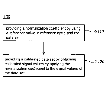
Fig. 1 represents a flow diagram illustrating an embodiment of the present
method
for calibrating a data set of a target analyte in a sample.
Fig. 2a represents amplification curves of three groups of raw data sets
obtained
respectively from three instruments without a hardware adjustment to show the
inter-
instrument and the intra-instrument variation of background signals.
Fig. 2b represents baseline subtracted amplification curves of three groups of
raw
data sets obtained respectively from three instruments without a hardware
adjustment and
analytical results of the inter- and the intra-instrument coefficient of
variation of the data
4
CA 03005600 2018-05-16
WO 2017/086762
PCT/KR2016/013423
sets.
Fig. 3a represents amplification curves of three groups of raw data sets
obtained
respectively from three instruments with a hardware adjustment to show the
inter-
instrument and the intra-instrument variation of background signals.
Fig. 3b represents baseline subtracted amplification curves of three groups of
raw
data sets obtained respectively from three instruments with a hardware
adjustment and
analytical results of the inter- and the intra-instrument coefficient of
variation of the data
sets.
Fig. 4a represents amplification curves of calibrated data sets obtained by
calibration
of three groups of raw data sets by specific background signal based
normalization method
(SBN) of present invention using common reference value, wherein the raw data
sets are
= obtained respectively from three instruments without a hardware
adjustment.
Fig. 4b represents baseline subtracted amplification curves of calibrated data
sets
obtained by calibration of three groups of raw data sets by the SBN using a
common
reference value, wherein the raw data sets are obtained respectively from
three
instruments without a hardware adjustment and analytical results of the inter-
and the
intra-instrument coefficient of variation of the calibrated data sets.
Fig. 5a represents amplification curves of calibrated data sets obtained by
calibration
of three groups of raw data sets by the SBN using a common reference value,
wherein the
raw data sets are obtained respectively from three instruments with a hardware
adjustment.
Fig. 5b represents baseline subtracted amplification curves of calibrated data
sets
obtained by calibration of three groups of raw data sets by the SBN using a
common
reference value, wherein the raw data sets are obtained respectively from
three
instruments with a hardware adjustment and analytical results of the inter-
and the intra-
instrument coefficient of variation of the calibrated data sets.
Fig. 6a represents amplification curves of calibrated data sets obtained by
calibration
of three groups of raw data sets by the SBN using an instrument-specific
reference value,
wherein the raw data sets are obtained respectively from three instruments
without a
5
CA 03005600 2018-05-16
WO 2017/086762
PCT/KR2016/013423
hardware, adjustment.
Fig. 6b represents baSeline subtracted amplification curves of calibrated data
sets
obtained by calibration of three groups of raw data sets by the SBN using an
instrument-
specific reference value, wherein the raw data sets are obtained respectively
from three
instruments without a hardware adjustment and analytical results of the inter-
and the
intra-instrument coefficient of variation of the calibrated data sets.
Fig. 7a represents amplification curves of calibrated data sets obtained by
calibration
of three groups of raw data sets by the SBN using an instrument-specific
reference value,
wherein the raw data sets are obtained respectively from three instruments
with a
hardware adjustment.
Fig. 7b represents baseline subtracted amplification curves of calibrated data
sets
obtained by calibration of three groups of raw data sets by the SBN using an
instrument-
specific reference value, wherein the raw data sets are obtained respectively
from three
instruments with a hardware adjustment and analytical results of the inter-
and the intra-
instrument coefficient of variation of the calibrated data sets.
Fig. 8a represents amplification curves of calibrated data sets obtained by
calibration
of three groups of raw data sets by the instrument blank signal subtraction
and specific
background signal based normalization the IBS-SBN method of the present
invention using a
common reference value, wherein the raw data sets are obtained respectively
from three
instruments without a hardware adjustment.
Fig. 8b represents baseline subtracted amplification curves of calibrated data
sets
obtained by calibration of three groups of raw data sets by the IBS-SBN using
a common
reference value, wherein the raw data sets are obtained respectively from
three
instruments without a hardware adjustment and analytical results of the inter-
and the
intra-instrument coefficient of variation of the calibrated data sets.
Fig. 9a represents amplification curves of calibrated data sets obtained by
calibration
of three groups of raw data sets by the IBS-SBN using a common reference
value, wherein
the raw data sets are obtained respectively from three instruments with a
hardware
adjustment.
6
CA 03005600 2018-05-16
WO 2017/086762
PCT/KR2016/013423
Fig. 9b represents baseline subtracted amplificatidn curves of calibrated data
sets
obtained by calibration of three groups of raw data sets by the IBS-SBN using
a common
reference value, wherein the raw data sets are obtained respectively from
three
instruments with a hardware adjustment and analytical results of the inter-
and the intra-
instrument coefficient of variation of the calibrated data sets.
Fig. 10a represents amplification curves of calibrated data sets obtained by
calibration of three groups of raw data sets by the IBS-SBN using an
instrument-specific
reference value, wherein the raw data sets are obtained respectively from
three
instruments without a hardware adjustment.
Fig. 10b represents baseline subtracted amplification curves of calibrated
data sets
obtained by calibration of three groups of raw data sets by the IBS-SBN using
an
instrument-specific reference value, wherein the raw data sets are obtained
respectively
from three instruments without a hardware adjustment and analytical results of
the inter-
and the intra-instrument coefficient of variation of the calibrated data sets.
Fig. 11a represents amplification curves of calibrated data sets obtained by
calibration of three groups of raw data sets by the IBS-SBN using an
instrument-specific
reference value, wherein the raw data sets are obtained respectively from
three
instruments with a hardware adjustment.
Fig. 11b represents baseline subtracted amplification curves of calibrated
data sets
obtained by calibration of three groups of raw data sets by the IBS-SBN using
an
instrument-specific reference value, wherein the raw data sets are obtained
respectively
from three instruments with a hardware adjustment and analytical results of
the inter- and
the intra-instrument coefficient of variation of the calibrated data sets.
Fig. 12a represents melting curves of three groups of raw melting data sets
obtained respectively from three instruments without a hardware adjustment.
Fig. 12b represents melting peaks obtained by plotting the derivatives of the
raw
melting data sets obtained respectively from three instruments without a
hardware
adjustment and analytical results of the inter- and the intra-instrument
coefficient of
variation of maximum derivatives of the data sets.
7
CA 03005600 2018-05-16
WO 2017/086762
PCT/KR2016/013423
Fig. 13a represents melting curves of three groups of raW melting data sets
obtained respectively from three instruments with a hardware adjustment.
Fig. 13b represents melting peaks obtained by plotting the derivatives of the
raw
melting data sets obtained respectively from three instruments with a hardware
adjustment and analytical results of the inter- and the intra-instrument
coefficient of
variation of maximum derivatives of the data sets.
Fig. 14a represents melting curves of calibrated melting data sets obtained by
calibration of three groups of raw melting data sets by the IBS-SBN using a
common
reference value and a reference temperature of 55 C as a reference cycle,
wherein the raw =
to melting
data sets are obtained respectively from three instruments without a hardware
adjustment.
Fig. 14b represents melting peaks obtained by plotting the derivatives of the
calibrated melting data sets obtained by calibration of three groups of raw
melting data
sets by the IBS-SBN using a common reference value and a reference temperature
of 55 C
as a reference cycle, wherein the raw melting data sets are obtained
respectively from
three instruments without a hardware adjustment and analytical results of the
inter- and
the intra-instrument coefficient of variation of maximum derivatives of the
data sets.
Fig. 14c represents melting peaks obtained by plotting the derivatives of the
calibrated melting data sets obtained by calibration of three groups of raw
melting data
sets by the IBS-SBN using a common reference value and a reference temperature
of 85 C
as a reference cycle, wherein the raw melting data sets are obtained
respectively from
three instruments without a hardware adjustment and analytical results of the
inter- and
the intra-instrument coefficient of variation of maximum derivatives of the
data sets.
Fig. 15a represents melting curves of calibrated melting data sets obtained by
calibration of three groups of raw melting data sets by the IBS-SBN using a
common
reference value and a reference temperature of 55 C as a reference cycle,
wherein the raw
melting data sets are obtained respectively from three instruments with a
hardware
adjustment.
Fig. 15b represents melting peaks obtained by plotting the derivatives of the
8
CA 03005600 2018-05-16
WO 2017/086762
PCT/KR2016/013423
calibrated melting data sets obtained by calibration of three groups of raw
melting data
sets by the IBS-SBN using a common reference value and a reference temperature
of 55 C
as a reference cycle, wherein the raw melting data sets are obtained
respectively from
three instruments with a hardware adjustment and analytical results of the
inter- and the
intra-instrument coefficient of variation of maximum derivatives of the data
sets.
Fig. 16a represents melting curves of calibrated melting data sets obtained by
calibration of three groups of raw melting data sets by the IBS-SBN using an
instrument-
specific reference value and a reference temperature of 55 C as a reference
cycle, wherein
the raw melting data sets are obtained respectively from three instruments
without a
hardware adjustment.
Fig. 16b represents melting peaks obtained by plotting the derivatives of the
calibrated melting data sets obtained by calibration of three groups of raw
melting data
sets by the IBS-SBN using, an instrument-specific reference value and a
reference
temperature of 55 C as a reference cycle, wherein the raw melting data sets
are obtained
respectively from three instruments without a hardware adjustment and
analytical results
of the inter- and the intra-instrument coefficient of variation of maximum
derivatives of the
data sets.
Fig. 17a represents melting curves of calibrated melting data sets obtained by
calibration of three groups of raw melting data sets by the IBS-SBN using an
instrument-
specific reference value and a reference temperature of 55 C as a reference
cycle, wherein
the raw melting data sets are obtained respectively from three instruments
with a
hardware adjustment.
Fig. 17b represents melting peaks obtained by plotting the derivatives of the
calibrated melting data sets obtained by calibration of three groups of raw
melting data
sets by the IBS-SON using an instrument-specific reference value and a
reference
temperature of 55 C as a reference cycle, wherein the raw melting data sets
are obtained
respectively from three instruments with a hardware adjustment and analytical
results of
the inter- and the intra-instrument coefficient of variation of maximum
derivatives of the
data sets.
9
CA 03005600 2018-05-16
WO 2017/086762
PCT/KR2016/013423
Fig. 18 represents a corriparative result of data sets obtaihed using probes
of
various concentrations and calibrated data sets obtained by the IBS-SBN using
various
reference values.
DETAILED DESCRIPTION OF THIS INVENTION
I. Method for calibrating a data set of a target analyte
In one aspect of this invention, there is provided a method for calibrating a
data set
of a target analyte in a sample comprising:
(a) providing a normalization coefficient for calibrating the data set;
wherein the data
set is obtained from a signal-generating process for the target analyte using
a signal-
generating means; wherein the data set comprises a plurality of data points
comprising
cycles of the signal-generating process and signal values at the cycles;
wherein the
normalization coefficient is provided by using a reference value, a reference
cycle and the
data set; wherein the reference cycle is selected from the cycles of the data
set; wherein
the reference value is an arbitrarily determined value; wherein the
normalization coefficient
is provided by defining a relationship between the reference value and a
signal value at a
cycle of the data set corresponding to the reference cycle; and
(b) providing a calibrated data set by obtaining calibrated signal values by
applying
the normalization coefficient to the signal values of the data set.
The present inventors have made intensive researches to develop novel
approaches
for calibrating a data set and more effectively reducing the inter- and intra-
instrument
variation among a plurality of data sets which represent the presence or
absence of target
analyte, for instance target nucleic acid molecule. As results, we have found
that the
calibrated data set can be obtained with accuracy and reliability by providing
a normalization
coefficient by using a reference value, a reference cycle and a data set and
applying the
normalization coefficient to the signal values of the plurality of data
points.
According to an embodiment, this approach is named herein as "Specific
Background
CA 03005600 2018-05-16
WO 2017/086762
PCT/KR2016/013423
signal based Normalization (SBN)" method, because a specific background signal
of a
specific cycle i.e., a reference cycle in background region is used for a
calibration.
The term used herein "normalization" refers to a process of reducing or
eliminating a
signal variation of a data set obtained from a signal-generating process. The
term used
herein "calibration" or "adjustment" refers to a correction of a data set,
particularly a
correction of a signal value of a data set, suitable for the aim of analysis.
The normalization
is one aspect of the calibration.
Fig. 1 represents a flow diagram illustrating an embodiment of the present
method
for calibrating a data set of a target analyte in a sample according to the
SBN method. The
present invention will be described in more detail as follows:
Step (a): Providing a normalization coefficient for calibrating a data
set(110)
According to the presertt method, a normalization coefficient for calibrating
a data set
is provided. The data set is obtained from a signal-generating process for a
target analyte
using a signal-generating means, and the data set comprises a plurality of
data points
comprising cycles of the signal-generating process and signal values at the
cycles.
The terms used herein a target analyte may include various materials (e.g.,
biological
materials and non-biological materials such as chemicals). Particularly, the
target analyte
may include biological materials such as nucleic acid molecules (e.g., DNA and
RNA),
proteins, peptides, carbohydrates, lipids, amino acids, biological chemicals,
hormones,
antibodies, antigens, metabolites and cells. More particularly, the target
analyte may include
nucleic add molecules. According to an embodiment, the target analyte may be a
target
nucleic acid molecule.
The term used herein "sample" may include biological samples (e.g., cell,
tissue and
fluid from a biological source) and non-biological samples (e.g., food, water
and soil). The
biological samples may include virus, bacteria, tissue, cell, blood (e.g.,
whole blood, plasma
and serum), lymph, bone marrow aspirate, saliva, sputum, swab, aspiration,
milk, urine,
stool, vitreous humour, sperm, brain fluid, cerebrospinal fluid, joint fluid,
fluid of thymus
gland, bronchoalveolar lavage, ascites and amnion fluid. When a target analyte
is a target
11
CA 03005600 2018-05-16
WO 2017/086762
PCT/ICR2016/013423
nucleic acid molecule, the satnple is subjected to a nucleic acid extraction
process. When the
extracted nucleic add is RNA, reverse transcription process is performed
additionally to
synthesize cDNA from the extracted RNA(Joseph Sambrook, et al., Molecular
Cloning, A
Laboratoty Manual, Cold Spring Harbor Laboratory Press, Cold Spring Harbor,
N.Y.(2001)).
The term used herein "signal-generating process" refers to any process capable
of
generating signals in a dependent manner on a property of a target analyte in
a sample,
wherein the property may be, for instances, activity, amount or presence (or
absence) of
the target analyte, in particular the presence of (or the absence of) an
analyte in a sample.
According to an embodiment, the signal-generating process generates signals in
a
dependent manner on the presence of the target analyte in the sample.
Such signal-generating ;process may include biological and chemical processes.
The
biological processes may include genetic analysis processes such as PCR, real-
time PCR,
microarray and invader assay, immunoassay processes and bacteria growth
analysis.
According to an embodiment, the signal-generating process includes genetic
analysis
processes. The chemical processes may include a chemical analysis comprising
production,
change or decomposition of chemical materials. According to an embodiment, the
signal-
generating process may be a PCR or a real-time PCR.
The signal-generating process may be accompanied with a signal change. The
term
"signal" as used herein refers to a measurable output. The signal change may
serve as an
indicator indicating qualitatively or quantitatively the property, in
particular the presence or
absence of a target analyte. Examples of useful indicators include
fluorescence intensity,
luminescence intensity, chemilum inescence
intensity, bioluminescence intensity,
phosphorescence intensity, charge transfer, voltage, current, power, energy,
temperature,
visaisity, light scatter, radioactive intensity, reflectivity, transmittance
and absorbance. The
most widely used indicator is fluorescence intensity. The signal change may
include a signal
decrease as well as a signal increase. According to an embodiment, the signal-
generating
process is a process amplifying the signal values.
The term used herein "signal-generating means" refers to any material used in
the
12
CA 03005600 2018-05-16
WO 2017/086762
PCT/KR2016/013423
generation of a signal indicating a property, more specifically the presence
or absence of the
target analyte which is intended to be analyzed.
A wide variety of the signal-generating means have been known to one of skill
in the
art. Examples of the signal-generating means may include oligonucleotides,
labels and
enzymes. The signal-generating means include both labels per se and
oligonucleotides with
labels. The labels may include a fluorescent label, a luminescent label, a
chemiluminescent
label, an electrochemical label and a metal label. The label per se like an
intercalating dye
may serve as signal-generating means. Alternatively, a single label or an
interactive dual
label containing a donor molecule and an acceptor molecule may be used as
signal-
generating means in the form of linkage to at least one oligonucleotide. The
signal-
generating means may comprise additional components for generating signals
such as
nucleolytic enzymes (e.g., 5'-nucleases and 3'-nucleases).
Where the present method is applied to determination of the presence or
absence of
a target nucleic acid molecule, the signal-generating process may be performed
in
accordance with a multitude of methods known to one of skill in the art. The
methods
include TaqManTm probe method (U.S. Pat. No. 5,210,015), Molecular Beacon
method (Tyagi
et al., Nature Biotechnology, 14 (3):303(1996)), Scorpion method (Whitcombe et
al., Nature
Biotechnology 17:804-807(1999)), Sunrise or Amplifluor method (Nazarenko et
al., Nucleic
Acids Research, 25(12):2516-2521(1997), and U.S. Pat. No. 6,117,635), Lux
method (U.S.
Pat. No. 7,537,886), CPT (Duck P, et al., Biotechniques, 9:142-148(1990)), LNA
method (U.S.
Pat. No. 6,977,295), Plexor method (Sherrill CB, et al., Journal of the
American Chemical
Society, 126:4550-4556(2004)), HybeaconsTm (D. J. French, et al., Molecular
and Cellular
Probes (2001) 13, 363-374 and U.S. Pat. No. 7,348,141), Dual-labeled, self-
quenched probe
(US 5,876,930), Hybridization probe (Bernard PS, et al., Clin Chem 2000, 46,
147-148),
PTOCE (PTO cleavage and extension) method (WO 2012/096523), PCE-SH (PTO
Cleavage
and Extension-Dependent Signaling Oligonucleotide Hybridization) method (WO
2013/115442) and PCE-NH (PTO Cleavage and Extension-Dependent Non-
Hybridization)
method (PCT/KR2013/012312) and CER method (WO 2011/037306).
13
CA 03005600 2018-05-16
WO 2017/086762
PCT/KR2016/013423
The term used herein "amplification" or "amplification reaction" refers to a
reaction
for increasing or decreasing signals. According to an embodiment of this
invention, the
amplification reaction refers to an increase (or amplification) of a signal
generated
depending on the presence of the target analyte by using the signal-generating
means. The
amplification reaction is accompanied with or without an amplification of the
target analyte
(e.g., nucleic acid molecule). Therefore, according to an embodiment of this
invention, the
signal-generating process is performed with or without an amplification of the
target nucleic
acid molecule. More particularly, the amplification reaction of present
invention refers to a
signal amplification reaction performed with an amplification of the target
analyte.
The data set obtained from an amplification reaction comprises an
amplification cycle.
The term used herein "cycle" refers to a unit of changes of conditions or a
unit of a
repetition of the changes of conditions in a plurality of measurements
accompanied with
changes of conditions. For example, the changes of conditions or the
repetition of the
changes of conditions include changes or repetition of changes in temperature,
reaction time,
reaction number, concentration, pH and/or replication number of a measured
subject (e.g.,
target nucleic acid molecule). Therefore, the cycle may include a condition
(e.g.,
temperature or concentration) change cycle, a time or a process cycle, a unit
operation cycle
and a reproductive cycle. A cycle number represents the number of repetition
of the cycle.
In this document, the terms "cycle" and "cycle number" are used
interchangeably.
For example, when enzyme kinetics is investigated, the reaction rate of an
enzyme is
measured several times as the concentration of a substrate is increased
regularly. In this
reaction, the increase in the substrate concentration may correspond to the
changes of the
conditions and the increasing unit of the substrate concentration may be
corresponding to a
cycle. For another example, when an isothermal amplification of nucleic acid
is performed,
the signals of a single sample are measured multiple times with a regular
interval of times
under isothermal conditions. In this reaction, the reaction time may
correspond to the
changes of conditions and a unit,of the reaction time may correspond to a
cycle. According
to another embodiment, as one of methods for detecting a target analyte
through a nucleic
acid amplification reaction, a plurality of fluorescence signals generated
from the probes
14
CA 03005600 2018-05-16
WO 2017/086762
PCT/KR2016/013423
hybridized to the target analyte are measured with a regular change of the
temperature in
the reaction. In this reaction, the change of the temperature may correspond
to the changes
of conditions and the temperature may correspond to a cycle.
Particularly, when repeating a series of reactions or repeating a reaction
with a time
interval, the term "cycle" refers to a unit of the repetition. For example, in
a polymerase
chain reaction (PCR), a cycle refers to a reaction unit comprising
denaturation of a target
nucleic acid molecule, annealing (hybridization) between the target nucleic
acid molecule
and primers and primer ext,ensiqn. The increases in the repetition of
reactions may
correspond to the changes of conditions and a unit of the repetition may
correspond to a
cycle.
According to an embodiment, where the target nucleic acid molecule is present
in a
sample, values (e.g., intensities) of signals measured are increased or
decreased upon
increasing cycles of an amplification reaction. According to an ernbodinient,
the amplification
reaction to amplify signals indicative of the presence of the target nucleic
acid molecule may
be performed in such a manner that signals are amplified simultaneously with
the
amplification of the target nucleic acid molecule (e.g., real-time PCR).
Alternatively, the
amplification reaction may be performed in such a manner that signals are
amplified with no
amplification of the target nucleic acid molecule [e.g., CPT method (Duck P,
et al.,
Biotechniques, 9:142-148 (1990)), Invader assay (U.S. Pat. Nos. 6,358,691 and
6,194,149)].
The target analyte may be amplified by various methods. For example, a
multitude of
methods have been known for amplification of a target nucleic acid molecule,
including, but
not limited to, PCR (polymerase chain reaction), LCR (ligase chain reaction,
see U.S. Pat. No.
4683195 and No. 4683202; A Guide to Methods and Applications (Innis et al.,
eds, 1990);
Wiedmann M, et al., "Ligase chain reaction (LCR)- overview and applications."
PCR Methods
and Applications 1994 Feb;3(4):551-64), GLCR (gap filling LCR, see WO
90/01069, EP
439182 and WO 93/00447), Q-beta (Q-beta replicase amplification, see Cahill P,
et al., Clin
Chem., 37(9):1482-5(1991), U.S. Pat. No. 5556751), SDA (strand displacement
amplification,
see G T Walker et al., Nucleic Acids Res. 20(7):1691-1696(1992), EP 497272),
NASBA
(nucleic acid sequence-based amplification, see Compton, J. Nature
350(6313):91-2(1991)),
CA 03005600 2018-05-16
WO 2017/086762
PCT/KR2016/013423
TMA (Transcription-Mediated Amplification, see Hofmann WP et al., J Clin
Virol. 32(4):289-
93(2005); U.S. Pat. No. 5888779).) or RCA (Rolling Circle Amplification, see
Hutchison C.A.
et al., Proc. Natl Acad. Sci. USA. 102:17332-17336(2005)).
According to an embodiment, the label used for the signal-generating means may
comprise a fluorescence, more particularly, a fluorescent single label or an
interactive dual
label comprising donor molecule and acceptor molecule (e.g., an interactive
dual label
containing a fluorescent reporter molecule and a quencher molecule).
According to an embodiment, the amplification reaction used in the present
invention
may amplify signals simultaneously with amplification of the target analyte,
particularly the
target nucleic acid molecule. According to Jn embodiment, the amplification
reaction is
performed in accordance with a PCR or a real-time PCR.
The data set obtained from a signal-generating process comprises a plurality
of data
points comprising cycles of the signal-generating process and signal values at
the cycles.
The term used herein "values of signals" or "signal values" means either
values of
signals actually measured at the cycles of the signal-generating process
(e.g., actual value
of fluorescence intensity processed by amplification reaction) or their
modifications. The
modifications may include mathematically processed values of measured signal
values (e.g.,
intensities). Examples of mathematically processed values of measured signal
values may
include logarithmic values and derivatives of measured signal values. The
derivatives of
measured signal values may include multi-derivatives.
The term used herein "data point" means a coordinate value comprising a cycle
and a
value of a signal at the cycle. The term used herein "data" means any
information
comprised in data set. For example, each of cycles and signal values of an
amplification
reaction may be data. The data points obtained from a signal-generating
process,
particularly from an amplification reaction may be plotted with coordinate
values in a
rectangular coordinate system. In the rectangular coordinate system, the X-
axis represents
cycles of the amplification reaction and the Y-axis represents signal values
measured at each
cycles or modifications of the signal values.
16
CA 03005600 2018-05-16
WO 2017/086762
PCT/KR2016/013423
The term used herein "data set" refers to a set of data points. The data set
may
include a raw data set which is a set of data points obtained directly from
the signal-
generating process (e.g., an aMplification reaction) using a signal-generating
means.
Alternatively, the data set may be a modified data set which is obtained by a
modification of
the data set including a set of data points obtained directly from the signal-
generating
process. The data set may include an entire or a partial set of data points
obtained from the
signal-generating process or modified data points thereof.
According to an embodiment of this invention, the data set may be a
mathematically
processed data set of the raw data set. In particular, the data set may be 6
baseline
subtracted data set for removing a background signal value from the raw data
set. The
baseline subtracted data set may be obtained by methods well known in the art
(e.g., US
8,560,240).
The term "raw data set" as used herein refers to a set of data points
(including cycle
numbers and signal values) obtained directly from an amplification reaction.
The raw data
set means a set of non-processed data points which are initially received from
a device for
performing a real-time PCR (e.g., thermocycler, PCR machine or DNA amplifier).
In an
embodiment of the present invention, the raw data set may include a raw data
set
understood conventionally by one skilled in the art. In an embodiment of the
present
invention, the raw data set may include a dataset prior to processing. In an
embodiment of
the present invention, the raw data set may include a dataset which is the
basis for the
mathematically processed data sets as described herein. In an embodiment of
the present
invention, the raw data set may include a data set not subtracted by a
baseline (no baseline
subtraction data set).
The method of the present invention may be a method for calibrating a single
data
set of a target analyte in a sample. Alternatively, the method for present
invention may be a
method for calibrating a plurality of data sets. According to an embodiment, a
data set of
the present invention may comprise a plurality of data sets. Particularly, The
plurality of data
sets is a plurality of data sets of same-typed target analytes.
17
CA 03005600 2018-05-16
WO 2017/086762
PCT/KR2016/013423
According to on embodiment, the data set of step (a) may be a data set which
is
removed of an instrument blank signal. Alternatively, the data set of step (a)
may be the
data set which is not removed of an instrument blank signal.
The term "1st calibrated data set" may be used herein in order to refer to the
modified data set in which an instrument blank signal is removed from the raw
data set. The
1st calibrated data set may be interpreted as a modified data set and is
distinguished from
the finally calibrated data set or the 2'd calibrated data set.
According to an embodiment, the instrument blank signal may be obtained by no
use
of the signal-generating means. Particularly, the instrument blank signal is a
signal detected
to from a
reaction performed without signal-generating means such as labels per se, or
labeled
oligonucleotides which generate a signal by the presence of the target
analyte. Because
such instrument blank signal is measured in the absence of the signal-
generating means, a
signal variation due to an instrument-to-instrument difference in ratios of
signals generated
per unit concentration of target analytes is not applied to the instrument
blank signal.
The instrument blank signal may be determined and applied in various
approaches.
For example, the separate instrument blank signals may be determined for
applying to their
corresponding instruments. A single instrument blank signal may be applied to
data sets
obtained by a single instrument and different instrument blank signals each
may be applied
to the data sets obtained each of their corresponding instruments.
Alternatively, different
instrument blank signals each may be determined for applying to each of wells
within a
single instrument. Each well within a single instrument may have its own
instrument blank
signal and different instrument blank signals each may be applied to data sets
obtained by
each of their corresponding wells within a single instrument.
The data set which is removed of an instrument blank signal may be the data
set in
which an instrument blank signal is removed in whole or in part. The term of
"removal"
means subtracting or adding a value of signal from/to a data set.
Particularly, the term
"removal" refers to subtraction of a value of signal from a data set. When an
instrument
blank signal has a negative value, it may be removed by adding a value of
signal.
According to an embodiment, the instrument blank signal may be obtained by no
use
18
CA 03005600 2018-05-16
WO 2017/086762
PCT/KR2016/013423
of the signal-generating means. Particularly, the instrument blank signal may
be measured
using an empty well, an empty tube, a tube containing water or a tube
containing a real-
time PCR reaction mixture without signal-generating means such as fluorescence
molecule
conjugated oligonucleotide. A measurement of an instrument blank signal may be
performed
together with a signal-generating process or may be performed separately from
a signal-
generating process.
According to an embodiment, an instrument blank signal may be removed in whole
in
such a manner that measurement of the instrument blank signal is performed
together with
a signal-generating process and the measured instrument blank signal is
subtracted from
to signal values of a data set obtained by the signal-generating process.
Alternatively, an instrument blank signal may be removed in part in such a
manner
that a certain value of a signal is subtracted from signal values of a data
set obtained by a
signal-generating process. The certain value of a signal may be any value so
long as a signal
corresponding to an instrument blank signal in a data set is reduced by the
subtraction of
the certain value of signal. For instance, the certain value of a signal may
be determined
based on a plurality of instrument blank signals measured from one instrument
or a plurality
of instruments. When it is troublesome to measure an instrument blank signal
for each
target analyte analysis experiment, an instrument blank signal may be removed
from data
sets in such a manner that a certain value of signal corresponding to a
portion of the
instrument blank signal is determined based on a plurality of instrument blank
signals
measured from one instrument or from a plurality of instruments and then the
determined
certain value of signal is subtracted from each of data sets.
Alternatively, the certain value of signal may be determined in such a range
that a
signal variation of a data set is reduced when the certain value of signal is
subtracted from
the data set and the signal values of the subtracted data set are calibrated
with ratio
according to the present method. As such, the data set reduced of an
instrument blank
signal may be provided by subtracting the certain value of signal which is a
portion of the
instrument blank signal without measurement of an instrument blank signal for
each
reaction.
19
CA 03005600 2018-05-16
WO 2017/086762
PCT/KR2016/013423
According to an embodiment, the method further comprises the step of
performing
the signal-generating process to obtain a data set of the target analyte in
the sample before
the step (a).
According to an embodiment, the data set of the target analyte may indicate
the
presence or absence of the target analyte in the sample. In this case, the
method provided
by the present invention is described as "a method for calibrating data set
representing the
presence or absence of a target analyte in a sample". The calibration of a
data set
representing the presence or absence of a target analyte in a sample is
performed
eventually for determining the presence or absence of a target analyte in a
sample. The
term used "determining the presence or absence of an analyte in a sample"
means
determining qualitatively or quantitatively the presence or absence of an
analyte in a sample.
According to an embodiment, the normalization coefficient may be provided by
using
a reference value, a reference cycle and the data set.
The reference cycle is selected from the cycles of the data set. The reference
value is
an arbitrarily determined value. The normalization coefficient is provided by
defining a
relationship between the reference value and a signal value at a cycle of the
data set
corresponding to the reference cycle.
The reference cycle is a cycle selected for determining a specific signal
value used for
providing a normalization coefficient with a reference value. The reference
cycle used for
providing a normalization coefficient may be selected arbitrarily from cycles
of the data set.
The reference cycle may encompass a reference temperature, a reference
concentration or a reference time depending on the meaning of the cycle. For
instance, a
reference temperature may be a reference cycle of melting data set, wherein
the unit of
cycle is temperature. In the description regarding melting data set, the terms
"reference
cycle" and "reference temperature" may be used interchangeably.
According to an embodiment, the reference cycle is selected from a reference
cycle
group of each data set, wherein the reference cycle group of each data set is
provided in
CA 03005600 2018-05-16
WO 2017/086762
PCT/KR2016/013423
the same Manner to each other.
According to an embodiment, the reference cycle is selected from a reference
cycle
group of each data set, wherein the reference cycle group is generated based
on an
identical rule. The iqentical rule may be applied equally to the determination
of the
reference cycle in all data sets.
The reference cycle group of each data set is provided in the same manner to
each
other. The reference cycle group may be determined by various approaches. For
example,
the reference cycle group may, comprise the cycles at which a similar level of
signal values is
measured. The reference cycle 6roup may comprise the cycles at which a
substantially
identical level of signal values is measured. the reference cycle group may
comprise the
cycles where the coefficient of variation of signal values is within 5%, 6%,
7%, 8%, 9%,
10%.
When the data set is plotted as a sigmoidal response shape, the reference
cycle
group may comprise the cycles before and/Or after the amplification region
(i.e., growth
phase). The region before the amplification region may be baseline region or
early stage
region. The region after the amplification region may be the plateau region or
late stage
region. The reference cycle group may comprise a single cycle wherein the
number of the
single cycle of each data set is identical to one another.
The number of the reference cycle(s) determined in each data set may be
identical to
one another. Alternatively, the number of the reference cycle(s) determined in
each data set
may be different from one another.
According to an embodiment, the plurality of data sets is calibrated by using
a
reference cycle or cycles selected from a reference cycle group which is
provided in the
same manner (a common rule or a pre-determined criterion) to each other.
According to an embodiment, the same manner (a common rule or a pre-determined
criterion) provides a reference group, wherein the normalization coefficients
calculated from
a data set with the reference cycle or cycles selected from the reference
group may be
21
CA 03005600 2018-05-16
WO 2017/086762
PCT/KR2016/013423
substantially identical or in a range of narrow standard deviation (e.g. 15%,
10%, 8%, 5%
or 4%).
According to an embodiment, when the data set comprises the plurality of data
sets,
an identical reference cycle is applied to a plurality of data sets to be
analyzed with regard
to an identical criterion. According to an embodiment, the plurality of data
sets is calibrated
=by using an identical reference cycle.
The signal variation of data sets used for intra or inter-comparison analysis
or
analyzed by the identical criterion such as the same threshold need to be
minimized. A
range of data sets to be analyzed with regard to an identical criterion may be
determined by
a purpose of analysis, such as, but not limited thereto, a plurality of data
sets obtained from
a target analyte, obtained from the same type of sample, or obtained by the
same reaction
mixture (e.g, the same fluorescent molecules or same probe) may be analyzed
with regard
to an identical criterion.
However, according to an embodiment, when the data set comprises a plurality
of
data sets, at least two data sets of the plurality of data sets are applied
with different
reference cycles from each other so long as the signal values of the different
reference
cycles are substantially identical.
Because a reference cycle is used for determining a specific signal value
which is
used for providing a normalization coefficient together with a reference
value, the reference
cycle would be selected from cycles of data set where the cycles are capable
of providing a
signal value.
The reference cycle may be a pre-determined cycle or may be determined by an
experiment. The reference cycle may be selected from cycles of a data set.
Specifically, the
reference cycle is selected from cycles in a region of a data set where
amplification of signal
is not sufficiently detected.
For example, when the data set is obtained by a nucleic acid amplification
process, it
is preferable that the reference cycle is selected within a background signal
region. The
22
CA 03005600 2018-05-16
WO 2017/086762
PCT/KR2016/013423
background region refers to an early stage of a signal-generating process
before
amplification of signal is sufficiently detected.
The background region may be determined by various approaches. For instance,
the
end-point cycle of the background region may be determined with a cycle of the
first data
point having a slope more than a certain threshold in the first derivatives of
the data set
obtained by a nucleic acid amplification process. Alternatively, the start-
point cycle of the
background region may be determined with a starting cycle of the first peak in
the first
derivatives of the data set obtained by a nucleic acid amplification process.
Otherwise, the
end-point cycle of the background region may be determined with a cycle of a
data point
to having a maximum curvature.
According to an embodiment, the amplification process of the signal value may
be a
process providing signal values of a background signal region and a signal
amplification
region and the reference cycle may be selected within the background signal
region. More
specifically, according to an embodiment, the signal-generating process may be
a
polymerase chain reaction (PCR) or a real-time polymerase chain reaction (real-
time PCR)
and the reference cycle may be selected within the background signal region
before a signal
amplification region of the polymerase chain reaction (PCR) or the real-time
polymerase
chain reaction (real-time PCR). The signal values of initial background region
of data sets
obtained by a plurality of PCRs or real-time PCRs using the same target
analyte under the
same reaction condition would have theoretically the same or at least similar
value, because
the signal values of initial background region may comprise very low level of
the signal value
generated by target analyte regardless of the concentration of the target
analyte. Therefore,
it is preferable that the reference cycle is selected within the background
signal region.
Therefore, the number of the reference cycles may be not more than 50, 40, 30,
25,
20, 19, 18, 17, 16, 15, 14, 13, 12, 11, 10, 9 or 8. The reference cycle of the
present
invention may be selected with avoiding an initial noise signal. The number of
the reference
cycles may be not less than 0, 1, 2, 3, 4, 5, 6 or 7. Particularly, the
reference cycle of the
present invention may be determined from cycles 1-30, 2-30, 2-20, 2-15, 2-10,
2-8, 3-30, 3-
23
CA 03005600 2018-05-16
WO 2017/086762
PCT/KR2016/013423
20, 3-15, 3-10, 3-9, 3-43, 4-8, or 5-8 in the background region.
According to an embodiment, the reference cycle may be a single reference
cycle. A
single cycle may be used as a reference cycle, and a signal value at the
reference cycle of a
data set may be used for providing a normalization coefficient. Alternatively,
according to an
embodiment, the reference cycle may comprise at least two reference cycles.
The reference cycle may comprise at least two reference cycles and the signal
values
at the cycles of the data set corresponding to the reference cycles may
comprise at least
two signal values.
A normalization coefficient for calibration may be provided by using a signal
value
which is calculated from the respective signal values at the cycles of the
data set
corresponding to the at least two reference cycles. Alternatively, at least
two normalization
coefficients may be provided by using the respective signal values at the
cycles of the data
set corresponding to the at least two reference cycles, and a normalization
coefficient for
calibration may be provided from the at least two normalization coefficients.
For example,
4th, 5th and 6th
cycles may be designated as reference cycles, and the average of the signal
values of 4th, 5th and 6th cycles of a data set may be used for providing a
normalization
coefficient. For another example, the 4th, 5th and 6th cycles may be
designated as the
reference cycles and the normalization coefficients for each reference cycle
may be provided
by using the respective signal values at the cycles of the data set
corresponding to the
reference cycles, and then the average of the provided normalization
coefficients may be
determined as the final normalization coefficient to be applied to the data
set.
According to an embodiment, when a reference cycle is selected within a range
of
cycles of a data set, the reference cycle is selected from the cycles at which
the signal
values of the data sets to be analyzed with regard to an identical criterion
would have the
same value or at least similar value at the reference cycle.
A signal value used for providing a normalization coefficient to be applied to
a
plurality of data points for the calibration of a data set is determined by a
reference cycle
24
CA 03005600 2018-05-16
WO 2017/086762
PCT/KR2016/013423
and the data set. Particularly, the normalization coefficient is provided by
defining a
relationship between the reference value and a signal value at a cycle of the
data set
corresponding to the reference cycle.
According to an embodiment, the method of present invention may further
comprises
the step of removing abnormal signals (e.g., spike signal or jump error) from
a data set
obtained by signal-generating process before the determination of the signal
value used for
providing a normalization coefficient from the reference cycle and the data
set.
A reference value is a value used =for providing a normalization coefficient.
A
reference value of the present invention refers to an arbitrary value that is
applied to a
reference cycle for the calibrations of signal values of a data set. The data
sets to be
analyzed by an identical criterion may be applied with the same reference
value. When the
data set to be calibrated is a plurality of data sets, the plurality of data
sets may be
calibrated by using an identical reference value and this is one of the
important features of
the embodiment of the present invention.
A reference value may be an arbitrarily determined value. Preferably, the
reference
value may be an arbitrarily determined value from a real number except zero.
When the
reference value is zero, the normalization coefficient cannot be determined.
As used herein,
"a reference value may be an arbitrarily determined value" means that a
reference value
may be determined non-limitedly so long as the presence of a target analyte in
a sample is
determined by the calibrated data set using the reference value. The reference
value may
be selected arbitrarily by an experimenter so long as the presence of a target
analyte in a
sample is determined by the calibrated data set using the reference value.
Therefore, the
reference value to be used for calibrating a data set may be determined within
a range of
signal values to be obtained at the reference cycle of the same-typed signal-
generating
processes as a signal-generating process by which the data set is obtained.
The reference
value may be obtained separately from a data set to be calibrated.
Specifically, the
reference value may be determined by a data set which is obtained from a
signal-generating
CA 03005600 2018-05-16
WO 2017/086762
PCT/KR2016/013423
process of the same-typed of target analyte to a target analyte to be
analyzed. Alternatively,
the reference value may be obtained from a group of data sets comprising a
data set to be
calibrated.
Preferably, a reference value may be the same-typed value as the values of a
data
set to be calibrated and may have the same unit or dimension as the data set
to be
calibrated. However, even though the reference value and the signal value of
the data set
may have different units or dimensions from each other or the reference value
has no unit
or dimension, a proper normalization coefficient for each reaction may be
provided using a
ratio of the reference value to the signal value of the data set to be
calibrated, such that a
calibrated data set may be obtained using the normalization coefficient for
each reaction.
According to an embodiment, the signal-generating process may be a plurality
of
signal-generating processes for the detection of the same type of target
analytes, the data
set may be a plurality of data sets and a reference values applied to each
data set may be
determined independently from another reference value. The expresion used
herein "the
reference values may be determined independently" means that a reference value
for a data
set of the plurality of data sets may be determined without consideration of a
reference
value for another data set. Accordingly, When the data set of present
invention comprises
the plurality of data sets, at least two data sets of the plurality of data
sets may be
calibrated by using different reference values from each other or all of the
data set may be
calibrated by using an identical reference value.
The plurality of signal-generating processes may be a plurality of signal-
generating
processes for the detection of the same type of target analytes (i.e, the same-
typed target
analytes). The same type of target analytes may be a plurality of target
analytes isolated
from the same sample. Alternatively, the same type of target analytes may be a
plurality of
target analytes which is isolated from the different samples but detected by
the same signal-
generating means (e.g., the same probes or same primers).
According to an embodiment, the plurality of signal-generating processes may
be a
plurality of signal-generating processes for the same-typed target analyte
performed in
different reaction environments. Signal-generating processes in different
reaction
26
CA 03005600 2018-05-16
WO 2017/086762
PCT/KR2016/013423
environments comprise various embodiments. Particularly, the signal-generating
processes
in different reaction environments may be a signal-generating processes
performed on
different instruments, performed in different wells or reaction tubes,
performed for different
samples, performed with target analytes of different concentrations, performed
with
different primers or probes, performed with different signal-generating dyes
or performed by
different signal-generating means.
According to an embodiment, the signal-generating process may comprise a
plurality
of signal-generating processes performed in different reaction vessels, and
the data set may
comprise a plurality of data sets obtained from the plurality of signal-
generating processes.
Da The plurality of signal-generating processes may be performed in
different reaction vessels.
The term used herein "reaction vessel" refers to a vessel or a portion of a
device at which a
reaction is processed by mixing a sample and signal-generating means (e.g.,
primers or
probes). The expression used herein "the plurality of signal-generating
processes may be
performed in different reaction vessels" means that a signal-generating
process is performed
using a signal-generating means and a sample that are separated from another
signal-
generating means and sample for another signal-generating process. For
example, the
signal-generating processes performed in a plurality of tubes or in a
plurality of wells of a
plate may correspond to the plurality of signal-generating processes. The
signal-generating
processes which are performed in the same reaction vessel but in different
times also may
correspond to the plurality of signal-generating processes.
The plurality of signal-generating processes may be classified into several
groups with
regard to reaction environments (e.g., an instrument used). Particularly, the
plurality of
signal-generating processes performed in different instruments may be
classified into
different groups depending on the instruments performed. The plurality of data
sets
obtained from signal-generating processes which were performed in different
instruments
may be calibrated by using an identical reference value or may be calibrated
by using
different reference values for more fine calibration.
According to an embodiment, the plurality of signal-generating processes may
be
27
CA 03005600 2018-05-16
WO 2017/086762
PCT/KR2016/013423
performed on different instruments from each other. When the instrument
analyzes a single
sample at one operation, the plurality of data sets obtained from this type of
the plurality of
signal-generating processes may be calibrated by using different reference
values each
other.
According to an embodiment, the plurality of data sets may be calibrated by
using an
identical reference value. According to an embodiment, the plurality of data
sets may be
calibrated by using an identical reference cycle.
When a plurality of data sets is calibrated by using an identical reference
value
(common reference value) which is applied to the plurality of data sets in
common, all of the
data sets are calibrated to have an identical signal value at a reference
cycle, thereby
reducing the signal variation of the data sets. Therefore, the normalization
coefficients for
data sets obtained from a plurality of signal-generating processes which is
different in
reaction environments may be obtained by using an identical reference value,
which is one
of the important features of the embodiment of the present invention.
Particularly, each
normalization coefficient for the data sets obtained from a plurality of
signal-generating
processes which is different in reaction environments may be obtained by using
an identical
reaction cycle and an identical reference value. According to an embodiment,
the plurality of
data sets obtained from different instruments may be calibrated by using an
identical
reference value.
According to an embodiment, the reference value is determined within the
average
standard deviation (SD) of signal values at the cycles of the plurality of
data sets
corresponding to the reference cycle. When the reference value is determined
within the
range described above, a plurality of data sets may be normalized with
minimizing the
difference between the data set and the calibrated data set.
However, the plurality of data sets may be calibrated by using different
reference
values. Different reference values may be applied to a plurality of data sets
to be analyzed
by an identical criterion. According to an embodiment, at least two data sets
of the plurality
28
CA 03005600 2018-05-16
WO 2017/086762
PCT/KR2016/013423
of data sets may be calibrated by using different reference values from each
other.
The plurality of data sets may be classified into several groups with regard
to reaction
environments (e.g., an instrument used), and by considering differences of the
reaction
environments, a reference value appropriated each group may be determined and
applied.
Through this process, the signal variation among the plurality of data sets
may be calibrated
more precisely.
Where all of the plurality of the data sets may be classified into respective
different
groups from one another, a respective reference value is applied to each of
the all data sets.
When at least two data sets of the plurality of data sets may be classified
into a group, a
respective reference value is applied to each Of the at least twO data sets.
For example, the
data sets obtained in different wells within an instrument may be classified
into the same
group and the data sets obtained from different instruments may be Classified
into different
groups. According to an embodiment, the different reference values may be
applied to the
data sets obtained using different instruments and the same reference value
may be applied
to the data sets obtained in different wells within an instrument. According
to an
embodiment, at least two data sets of the plurality of data sets may be
calibrated by using
different reference values from each other wherein the at least two data sets
may be
obtained using different instruments from each other.
According to an embodiment, the signal-generating process may be a plurality
of
signal-generating processes for the same type of target analyte performed in
different
reaction vessels, the data set may comprise a plurality of data sets obtained
from the
plurality of signal-generating processes, and at least two data sets of the
plurality of data
sets are calibrated by using different reference values from each other. For
instance, to
calibrate an inter-instrument signal variation more precisely, an instrument-
specific standard
data set of each instrument and its total signal change value may be obtained
and then a
reference value to be applied to a data set obtained by using a corresponding
instrument
may be determined using the total signal change value, which is another
feature of the
embodiment of the present invention.
29
CA 03005600 2018-05-16
WO 2017/086762
PCT/KR2016/013423
The inter-instrument variation may be a signal variation between the separate
data
sets which are obtained by the signal-generating processes for the identical
target analyte
performed on the respective different instruments. Alternatively, the inter-
instrument
variation may be a signal variation between the separate data sets which are
obtained by
independent operations of the signal-generating processes for the identical
target analyte on
the identical instrument. For example, the independent operations of the
signal-generating
processes for the identical target analyte may be performed on the identical
instrument with
an operation time interval. In this case, the independent operation of an
instrument may be
considered as an instrument.
According to an embodiment, even though at least two data sets of the
plurality of
data sets may be calibrated by using different reference values, the at least
two data sets of
the plurality of data sets may be calibrated by using an identical reference
cycle.
According to an embodiment, the reference value is determined by (i) a ratio
of a
total signal change value of a standard data set to a reference total signal
change value;
wherein the standard data set is obtained by using a reaction site which is
identical to that
used for obtaining the data set from the signal-generating process for the
target analyte;
wherein the reference total signal change value is determined by one or more
data sets
comprising a data set obtained from a signal-generating process using a
reaction site which
is different from that used for obtaining the data set from the signal-
generating process for
the target analyte and (ii) the standard data set. Particularly, a signal
value at a reference
cycle of a standard data set may be calibrated using a ratio of a total signal
change value of
a standard data set to a reference total signal change value, followed by
determining a
reference value from the signal value at the reference cycle of the calibrated
standard data
set.
A reference value may be determined using a reference total signal change
value and
a total signal change value of a standard data set.
According to an embodiment, the standard data set is obtained by using a
reaction
site which is identical to that used for obtaining the data set from the
signal-generating
CA 03005600 2018-05-16
WO 2017/086762
PCT/KR2016/013423
process for the target analyte.
The reaction site is a physical space in which a process or a reaction of the
sample is
performed. The reaction site may include an instrument (e.g., PCR instrument)
and a part of
an instrument (e.g., reaction well configured in PCR instrument). The reaction
site is
configured for a target analyte detection e.g., the PCR amplification.
The standard data set may be a data set obtained by performing a signal-
generating
process for a target analyte of known concentration. The standard data set may
be obtaihed
using an identical well(s) or instrument to that for obtaining the data set
from the signal-
generating process for the target analyte.
According to an embodiment, the standard data set may be obtained separately
from
a data set of a target analyte to be calibrated. When a calibration ratio for
an instrument is
calculated based on a standard data set obtained using the instrument, a
signal-generating
process for the standard data set is not necessarily performed by a reaction
under the same
conditions as reaction conditions by which a data set of a target analyte in a
sample is
obtained.
According to another embodiment, the standard data set may be obtained
together
with the data set of the target analyte to be calibrated. The standard data
set may be
obtained by a reaction performed under the same reaction conditions as
reaction conditions
by which a data set of a target analyte in a sample is obtained. A fine
calibration for
compensating a signal variation found in each instrument run may be achieved.
Since the standard data set is a data set for a target analyte of known
concentration,
the standard data set can be used for determining a reference value by
comparative analysis
of the common factors between the standard data set and another data set for a
target
analyte of the same concentration as the known concentration. Specifically,
the target
analyte of known concentration may be a target analyte of a standard
concentration. The
common factors may be those which theoretically have constant values when an
identical
signal-generating process is performed under an identical condition. The
common factor
31
CA 03005600 2018-05-16
WO 2017/086762
PCT/KR2016/013423
may be, for instance, a total signal change value, a cycle number of a first
data point having
a signal value more than a threshold or a signal value at a cycle in baseline
region.
According to an embodiment, the data set may be calibrated by using a total
signal
change value as one of the common factor. The term used herein "total signal
change value"
means a signal change amount (increased or decreased) of the data set. The
total signal
change value may be a signal change amount (increased or decreased) of the
entire data
set or may be a signal change amount (increased or decreased) of a partial
region of the
data set. For example, the total signal change value may be a signal change
value at the
cycle having the greatest signal change value. Particularly, the total signal
change value may
be a difference between a signal value of baseline and a maximum signal value
of the data
set or a difference between a signal value of baseline and a signal value of
the last cycle of
the data set.
Meanwhile, when the total signal change value is determined within a region of
the
data set, the total signal change value may be a difference between the first
cycle and the
last cycle of the region of the data set or a difference between the maximum
signal value
and the minimum signal value of the region of the data set. Constant total
signal change
values may be obtained theoretically from the same or different instruments
when signal-
generating processes are performed using target analytes of an identical
concentration
under an identical condition. Therefore, the calibration based on the total
signal change
zo value may reduce a variation between a plurality of the data sets.
A reference total signal change value refers to a total signal change value
used in
determining a normalization coefficient in comparison with a total signal
change value of a
standard data set.
According to an embodiment, the reference total signal change value is may be
determined by one or more data sets comprising a data set obtained from a
signal-
generating process using the reaction site which is different from that used
for obtaining the
data set from the signal-generating process for the target analyte.
Specifically, the reference total signal change value may be determined by the
data
32
CA 03005600 2018-05-16
WO 2017/086762
PCT/KR2016/013423
set obtained from a signal-generating process using the reaction site which is
different from
that used for obtaining the data set from the signal-generating process for
the target
analyte together with the data set obtained from a signal-generating process
using the
reaction site which is identical to that used for obtaining the data set from
the signal-
s generating process for the target analyte.
More specifically, the reference total signal change value may be determined
by the
data set obtained from a signal-generating process using the reaction site
which is different
from that used for obtaining the data set from the signal-generating process
for the target
analyte.
to
The reference total signal change value may be a total signal change value
obtained
separately from the standard data set.
According to an embodiment, the reference total signal change value may be a
pre-
determined total signal change value. The reference total signal change value
may be
15 .. obtained by using a reference (or standard) vessel(s) or instrument(s)
with substantially
identical standard material use used for obtaining the total change value of
the standard
data set.
The reference total signal change value of the present invention may be
determined
by a data set obtained from a signal-generating process for the target analyte
of known
20 concentration. Alternatively, the reference total signal change value of
the present invention
may be calculated from total signal change values of a plurality of data sets
obtained from a
plurality of signal-generating processes for the target analyte of known
concentration. In
this case, the reference total signal change value is an average or median
value of a
plurality of data sets obtained from a plurality of signal-generating
processes for the target
25 analyte of known concentration or may be predetermined by an
experimenter based on the
results of a plurality of signal-generating processes for the target analyte
of known
concentration.
Alternatively, according to an embodiment, when the standard data set is a
plurality
of standard data sets, the reference total signal change value may be
determined from the
33
CA 03005600 2018-05-16
WO 2017/086762
PCT/KR2016/013423
plurality of standard data sets. For instance, one of the total signal change
values of the
plurality of standard data sets may be determined as a reference total signal
change value.
Alternatively, an average or median value of the total signal change values of
the plurality of
standard data sets may be determined as a reference total signal change value.
According to an embodiment, the reference value may be determined within a
range
of a plurality of signal values at reference cycles of a plurality of data
sets to be analyzed
with regard to an identical criterion. When the reference value is determined
within a range
of a plurality of signal values at reference cycles of a plurality of data
sets to be analyzed
with regard to an identical criterion, the plurality of data sets may be
calibrated with
minimizing difference between the data set and the calibrated data set.
_ _
According to an embodiment, the normalization coefficient for a data set may
be
provided by using a reference value and a reference cycle and the data set.
More
particularly, the normalization coefficient may be provided by using a
reference value and a
signal value at a cycle of the data set to be calibrated wherein the cycle is
corresponding to
the reference cycle. The normalization coefficient may be a value applied to a
plurality of
data points of a data set obtained from a reaction, thereby calibrating the
data set.
When the data set comprises the plurality of data sets, the plurality of data
sets may
be obtained from the plurality of signal-generating processes in different
reaction vessels.
The normalization coefficient may be provided for each data set of the
plurality of data sets.
The plurality of data sets may be calibrated by applying the normalization
coefficients. For
reducing signal variation shown between data sets to be analyzed by an
identical criterion,
the normalization coefficient appropriate to the data set is provided by the
present method.
The normalization coefficient is applied to signal values at a plurality of
data points of the
data set, thereby obtaining calibrated signal values to provide a calibrated
data set.
The normalization coefficient may be provided by using a reference value, a
reference
cycle and the data set. The normalization coefficient may be provided by
defining a
relationship between the reference value and a signal value at a cycle of the
data set
34
CA 03005600 2018-05-16
WO 2017/086762
PCT/KR2016/013423
corresponding to the reference cycle. The relationship between the reference
value and a
signal value at a cycle of the data set corresponding to the reference cycle
may be defined
by various ways, for example, the relationship may be defined mathematically.
The signal
value at the cycle of the data set corresponding to the reference cycle (i.e.,
at the reference
cycle-corresponding cycle of the data set) may be a signal value without
modification or may
be a signal value modified mathematically. Particularly, the relationship
between the
reference value and a signal value at a cycle of the data set corresponding to
the reference
cycle may be a difference between the reference value and a signal value at
the cycle of the
data set corresponding to the reference cycle. More particularly, the
difference between the
reference value and a signal value at the cycle of the data set corresponding
to the
reference cycle may be a ratio of the signal value at the cycle of the data
set corresponding
to the reference cycle to the reference value.
The cycle of the data set corresponding to the reference cycle is a reference
cycle-
corresponding cycle of the data set. According to an embodiment, the signal
value of a
reference cycle-corresponding cycle of the data set may be a single signal
value.
Alternatively, according to an embodiment, the signal value of a reference
cycle-
corresponding cycle of the data set may be a plurality of signal values.
The normalization coefficient may be provided by defining a relationship
between the
reference value and a signal value or by defining a relationship between the
reference value
and a plurality of signal values. The plurality of signal values may be
obtained at a reference
cycle or a plurality of reference cycles.
When the normalization coefficient is provided by a reference value and a
signal
value at the reference cycle-corresponding cycle of the data set, the
normalization
coefficient may be provided by a ratio of the signal value at the reference
cycle-
corresponding cycle of the data set to the reference value.
When the normalization coefficient is provided by a reference value and a
plurality of
signal values at the reference cycle-corresponding cycles of the data set, the
plurality of
signal values at the reference cycle-corresponding cycle of the data set may
be designated
by a plurality of reference cycles or a reference cycle.
CA 03005600 2018-05-16
WO 2017/086762 .
PCT/KR2016/013423
For example, when 3rd cycle is designated as a reference cycle, the plurality
of signal
values at the reference cycle-corresponding cycle may coMprise a_signal value
at 3'd cycle
and signal values at the cycles which are positioned one cycle before/after
the 3rd cycle. For
another example, when 2nd, 3rd and 4tn cycles are designated as reference
cycles, the
plurality of signal values at the reference cycle-correspondin cycle may
comprise signal
values at 2nd, 3rd and 4th cycle which are the reference cycle-corresponding
cycles.
The relationship between the plurality of signal values designated by
reference
cycle(s) and a reference value may be defined by various ways. For example,
the
relationship between the plurality of signal values and a reference value may
be defined by
a ratio of an average, median, minimum or maximum value of the plurality of
signal values
or an average value of threshold-below signal values of the plurality of
signal values to the
reference value. Preferably, the relationship between the plurality of signal
values
designated by reference cycle(s) and a reference value may be defined by a
ratio of an
average value of the Olurality of signal values to the reference value. When
the plurality of
signal values is used to provide the normalization coefficient, the influence
of an abnormal
signal value on calibration of a data set becomes negligible.
For example, when a signal value at the reference cycle-corresponding cycle of
the
data set is 0 (zero), all of the calibrated signal values of the data 'set may
have the same
value. The occurrence of such erroneous result may be much more reduced by
using a
plurality of signal values for providing the normalization coefficient than by
using a single
signal value. According to an embodiment, when a normalization coefficient is
0 (zero), all or '
some of signal values for providing the normalization coefficient may be
changed to other
signal values.
According to an embodiment, the normalization coefficient is provided by using
a
reference value and a signal value at the reference cycle-corresponding cycle
of the data set.
The normalization coefficient may be calculated by following mathematical
equation:
[Normalization coefficient = a signal value at the cycle of the data set
corresponding
36
CA 03005600 2018-05-16
WO 2017/086762
PCT/KR2016/013423
to the reference cycle / reference value]
For instance, the normalization coefficient may be calculated as 1.48, when a
data set
obtained by performing a real-time PCR for detection of a target analyte is
calibrated on
conditions that (a) the 5th cycle is designated as a reference cycle; (b) the
value of 9000 is
designated as a reference value; (c) the signal value at the cycle of the data
set
corresponding to the reference cycle is the value of 13,285 and (d) the
relationship between
the signal value at the reference cycle-corresponding cycle of the data set
and the reference
value is a ratio of the signal value at the reference cycle-corresponding
cycle of the data set
to the reference value. A calibrated data set may be provided by obtaining
calibrated signal
to values by
applying the normalization coefficient (1.48) to the signal values of the
plurality of
data points.
According to an embodiment, the normalization coefficient may be provided by
defining a ratio of a signal value at the reference cycle-corresponding cycle
of the data set
to the reference value. The normalization coefficient may be calculated by
following
mathematical equation:
[Normalization coefficient = a X (a signal value at the cycle of the data set
corresponding to the reference cycle / reference value)].
The a may be a real number except for 0 (zero), preferably, may be the number
of 1.
The a is a constant for adjusting a normalization coefficient properly when
the reference
value is determined dependent on other factors. A signal level of a reaction
may be
controllable through calibration of signal values of a data set with adjusting
the reference
value or the value of a, thereby controlling an amount of a reaction mixture
used for signal-
generating process.
All of data points of a data set may be calibrated by using an identical
normalization
coefficient in accordance with an identical mathematical equation.
Alternatively, all or a
portion of data points of a data set may be calibrated by using different
normalization
coefficients respectively or by using an identical normalization coefficient
in accordance with
different mathematical equations.
37
CA 03005600 2018-05-16
WO 2017/086762
PCT/KR2016/013423
Step (b): Providing a calibrated data set by applying a normalization
coefficient
(S120)
A calibrated data set may be provided by obtaining calibrated signal values by
applying the normalization coefficient to the signal values of the data set.
Particularly, a
calibrated data set may be provided by obtaining calibrated signal values by
applying the
normalization coefficient to the signal values of the plurality of data
points.
The normalization coefficient may be applied to the signal values of the data
set by
to various approaches.
When the normalizatiOn coefficient is provided by the ratio of the signal
value at the
reference cycle-corresponding cycle of the data set to the reference value, a
calibrated data
set may be provided by obtaining calibrated signal values.
According to an embodiment, the calibrated signal value is obtained by using
the
following mathematical equation 1:
Equation 1
Calibrated signal value = signal value / normalization coefficient
The signal value of equation 1 is uncalibrated signal value. The uncalibrated
signal
value refers to a signal value of a data set before the data set is calibrated
by the
normalization coefficient. Therefore, the uncalibrated signal value may be a
measured signal
value or a processed signal value of the measured signal value. The process
may be a
process performed independently from a calibration process using the
normalization
coefficient. For example, the signal value processing may be performed by
adding or
subtracting a certain amount of value to or from the signal value.
Particularly, the process
may be removing an instrument blank signal in whole or in part from the
measured signal
value.
The calibrated signal value refers to a signal value calibrated by the
normalization
coefficient. The calibrated data set may be provided by using the calibrated
signal value for
the signal value of the data set without further calibration.
38
CA 03005600 2018-05-16
WO 2017/086762
PCT/KR2016/013423
Alternatively, the calibrated data set may be provided by using the calibrated
signal
value for the signal value of the data set with further modification. For
instance, the signal
value calibrated by the normalization coefficient may be further calibrated by
adding or
subtracting a certain amount of value to or from the calibrated signal value.
Particularly, the
.. signal value calibrated by the normalization coefficient may be further
calibrated by
subtracting baseline signal value.
According to an embodiment, the calibrated data set is used for qualitative or
quantitative detection of the target analyte in the sample.
According to an embodiment, the data set of the present invention may be
obtained
from a signal-generating process for the target analyte using a signal-
generating means
without a reference dye, which is one of the features of the embodiment of the
present
invention. According to a conventional technology, a reference dye is
contained in a reaction
mixture for calibration (see W02012/083235). This prior art may have some
limitations or
.. shortcomings.
Introducing the reference dye into a reaction mixture may increase the
possibility of
an interference phenomenon between the reference dye and other) dyes used for
determining the presence of target analyte. In contrast, the present invention
can calibrate
a data set without introducing the reference dye into a reaction mixture
comprising signal-
.. generating means.
In the method of the present invention, the data set is capable of being
calibrated by
using the signal value of a target analyte without introducing the reference
dye into a
reaction mixture comprising signal-generating means, whereby it is possible to
calibrate the
data set more precisely and effectively than conventional method using the
reference dye
together with signal-generating means and to overcome various issues
associated with
variations in analytical results.
In Example described below, the CVs (coefficient of variation) of the inter-
and intra-
instrument variations of two groups of data sets were calculated and compared.
The data
39
CA 03005600 2018-05-16
WO 2017/086762
PCT/KR2016/013423
sets of group 1 were obtained by calibrating raw data sets according to the
method of the
present invention wherein the raw data sets were obtained by a real-time PCR
using three
instruments without a hardware adjustment. The data sets of group 2 were
obtained by the
same real-time PCR using three instruments with a hardware adjustment.
Furthermore, the CVs of the inter- and intra-instrument variations of two
groups of
melting data sets were calculated and compared. The melting data sets of group
1 were
obtained by calibrating raw melting data sets according to the method of the
present
invention wherein the raw melting data sets were obtained by performing a
melting analysis
using products of a real-time PCR using three instruments without a hardware
adjustment.
The melting data sets of group 2 were obtained by performing a melting
analysis using
products of a real-time PCR using three instruMents with a hardware
adjustment.
As a result, it was verified that the CVs (coefficient of variation) of the
inter- and
intra-instrument variations of the data sets or the melting data sets of group
1 is much
smaller than those of the data sets or the melting data sets of group 2. As
such, it would be
understood that the method of the present invention may be an alternative
solution of a
hardware adjustment not only for an amplification data set but also for a
melting data set.
Meanwhile, according to the method of the present invention, a level of signal
values
of a data set may be controlled by modulating the reference value. As a
result, a normalized
data set with statistical significance and may be obtained even when a small
amount of
signal-generating means (e.g., primers and probes) is used, finally
determining the presence
or absence of a target analyte in a sample.
According to an embodiment, the reference value may be selected to be higher
than
a maximum signal value of a baseline of the data set; wherein the signal-
generating process
may be a plurality of signal-generating processes for the same-typed target
analyte
performed in different reaction environments; wherein the data set is a
plurality of data sets;
wherein the plurality of data sets is calibrated by using an identical
reference cycle and an
identical reference value.
The reference value may be selected to be higher than a maximum signal value
of a
CA 03005600 2018-05-16
WO 2017/086762
PCT/KR2016/013423
baseline of the data set such that the ratio of the reference value to a
maximum signal value
of a baseline of the data set may become, not limited to, 1.1, 1.2, 1.3, 1.4,
1.5, 1.6, 1.7, 1.8,
1.9, 2, 3, 4, 5, 6, 7, 8, 9, 10, 15, 20, 30, 40, 50, 60, 70, 80, 90, 100, 200,
300, 400, and 500.
Interestingly, we have found that the present invention can minimize a signal
variation of a plurality of data sets along with increasing the level of
signal values of a
plurality of data sets to a desirable level.
In Example described below, two groups of data sets were compared. The data
sets
of group 1 were obtained by using various concentrations of signal-generating
means such
that the data sets of group 1 comprise data sets having various levels of
signal values. The
data sets of group 2 were obtained in such a manner that a raw data set was
obtained by
using low concentration of signal-generating means, followed by calibrating
the raw data set
using a plurality of reference values adjusted to calibrate the level of
signal values of the
raw data set to reach the various levels of signal values of data sets of
group 1. As a result, .
it was verified that data sets of groups 1 and 2 exhibited similar patterns of
an aMplification
curve and similar Ct values.
Furthermore, we verified that the CV of the calibrated raw data set obtained
using
low concentration of signal-generating means was substantially identical to
that of the pre-
calibrated raw data.
II. Storage Medium, Device and Computer Program
In another aspect of this invention, there is provided a computer readable
storage
medium containing instructions to configure a processor to perform a method
for calibrating
a data set of a target analyte in a sample, the method comprising:
(a) providing a normalization coefficient for calibrating the data set;
wherein the data
set is obtained from a signal-generating process for the target analyte using
a signal-
generating means; wherein the data set comprises a plurality of data points
comprising
cycles of the signal-generating process and signal values at the cycles;
wherein the
normalization coefficient is provided by using a reference value, a reference
cycle and the
41
CA 03005600 2018-05-16
WO 2017/086762
PCT/KR2016/013423
data set; wherein the reference cycle is selected from the cycles of the data
set; wherein
the reference value is an arbitrarily determined value; wherein the
normalization coefficient
is provided by defining a relationship between the reference value and a
signal value at a
cycle of the data set corresponding to the reference cycle; and
(b) providing a calibrated data set by obtaining calibrated signal values by
applying
the normalization coefficient to the signal values of the data set.
In another aspect of this invention, there is provided a computer program to
be
stored on a computer readable storage medium to configure a processor to
perform a
to method for calibrating a data set of a target analyte in a sample, the
method comprising:
(a) providing a normalization coefficient for calibrating the data set;
wherein the data
set is obtained from a signal-generating process for the target analyte using
a signal-
generating means; wherein the data set comprises a plurality of data points
comprising
cycles of the signal-generating process and signal values at the cycles;
wherein the
normalization coefficient is provided by using a reference value, a reference
cycle and the
data set; wherein the reference cycle is selected from the cycles of the data
set; wherein
the reference value is an arbitrarily determined value; wherein the
normalization coefficient
is provided by defining a relationship between the reference value and a
signal value at a
cycle of the data set corresponding to the reference cycle; and
(b) providing a calibrated data set by obtaining calibrated signal values by
applying
the normalization coefficient to the signal values of the data set.
The program instructions are operative, when performed by the processor, to
cause
the processor to perform the present method described above. The program
instructions for
performing the method for calibrating a data set of a target analyte in a
sample may
comprise an instruction to provide a normalization coefficient for calibrating
the data set by
using a reference value, a reference cycle and the data set; and an
instruction to provide a
calibrated data set by obtaining calibrated signal values by applying the
normalization
coefficient to the signal values of the data set.
42
CA 03005600 2018-05-16
WO 2017/086762
PCT/KR2016/013423
The present Method described above is implemented in a processor, such as a
processor in a stand-alone computer, a network attached computer or a data
acquisition
device such as a real-time PCR machine.
The types of the computer readable storage medium include various storage
medium
such as CD-R, CD-ROM, DVD, flash memory, floppy disk, hard drive, portable
HDD, USB,
magnetic tape, MINIDISC, nonvolatile memory card, EEPROM, optical disk,
optical storage
medium, RAM, ROM, system memory and web server.
The data set may be received through several mechanisms. For example, the data
set
may be acquired by a processor resident in a PCR data acquiring device. The
data set may
be provided to the processor in a real time as the data set is being
collected, or it may be
stored in a memory unit or buffer and provided to the processor after the
experiment has
been completed. Similarly, the data set may be provided to a separate system
such as a
desktop computer system via .a network connection (e.g., LAN, VPN, intranet
and Internet)
or direct connection (e.g., USB or other direct wired or wireless connection)
to the acquiring
is device,
or provided on a portable medium such as a CD, DVD, floppy disk, portable HDD
or
the like to a stand-alone computer system. Similarly, the data set may be
provided to a
server system via a network connection (e.g., LAN, VPN, intranet, Internet and
wireless
communication network) to a client such as a notebook or a desktop computer
system.
The instructions to configure the processor to perform the present invention
may be
included in a logic system. The instructions may be downloaded and stored in a
memory
module (e.g., hard drive or other memory such as a local or attached RAM or
ROM),
although the instructions can be provided on any software storage medium such
as a
portable HDD, USB, floppy disk, CD and DVD. A computer code for implementing
the
present invention may be implemented in a variety of coding languages such as
C, C++,
Java, Visual Basic, VBScript, JavaScript, Pen i and XML. In addition, a
variety of languages
and protocols may be used in external and internal storage and transmission of
data and
commands according to the present invention.
In still further aspect of this invention, there is provided a device for
calibrating data
43
CA 03005600 2018-05-16
WO 2017/086762
PCT/KR2016/013423
set of a target analyte in a sample, comprising (a) a computer processor and
(b) the
computer readable storage medium described above coupled to the computer
processor.
According to an embodiment, the device further comprises a reaction vessel to
accommodate the sample and signal-generating means, a temperature controlling
means to
control temperatures of the reaction vessel and/or a detector to detect
signals at
amplification cycles.
According to an embodiment, the computer processor permits not only to receive
values of signals at cycles but also to analyze a sample or data set or obtain
a calibrated
data set of a target analyte in a sample. The processor may be prepared in
such a manner
that a single processor can do all performances described above.
Alternatively, the processor
unit may be prepared in such a manner that multiple processors do multiple
performances,
respectively.
According to an embodiment, the processor may be embodied by installing
software
into conventional devices for detection of target nucleic acid molecules (e.g.
real-time PCR
device).
According to an embodiment, a calibrated data set is provided in such a manner
that
data set of a target analyte is obtained and the normalization coefficient is
provided by using
an arbitrarily determined reference value, a reference cycle and the data set,
follow by
obtaining calibrated signal values by applying the normalization coefficient
to the signal
values of the data set.
A reference value and a reference cycle may be arbitrarily determined by users
or
system suppliers. Alternatively, a reference value and a reference cycle may
be determined
by a device of the present invention. For example, the device of the present
invention which
collecting a plurality of data sets may be capable of determining a reference
cycle from
.. cycles in a background region regarding signal values of the accumulated
plurality of data
sets. Furthermore, the device of the present invention may be capable of
determining a
reference value within the average standard deviation (SD) of signal values
at the cycles
of the plurality of data sets corresponding to the reference cycle regarding
signal values of
the accumulated plurality of data sets. In addition, the device of the present
invention may
44
CA 03005600 2018-05-16
WO 2017/086762
PCT/KR2016/013423
be capable of determining a reference value regarding a ratio of a standard
data set to a
reference standard data set and a signal value of the reference cycle of the
standard data
set.
The features and advantages of this invention will be summarized as follows:
(a) According to the present invention, a data set is calibrated conveniently
by
applying a normalization coefficient to the data set to be calibrated such
that the inter- and
intra-instrument signal variations of data sets are reduced effectively.
Particularly, not only
the inter-instrument signal variations but also the intra-instrument signal
variations between
signal-generating processes caused by performing signal-generating processes
in different
positions (e.g., different reaction vessels or different wells) within an
instrument are
reduced, thereby the data set is capable of being analyzed with a high
accuracy and
reproductively.
(b) The present invention needs not a reference dye. More interestingly, the
present
method may calibrate a data set in more accurate and more economic manner than
conventional signal calibration methods using a reference dye. For reducing
inter-
instrument variation, the conventional calibration methods using the reference
dye demand
that the inter-instrument variation of an optical channel for detecting the
reference dye and
the inter-instrument variation of an optical channel for detecting a target
analyte have to be
the same. Therefore, the conventional calibration methods may not successfully
solve
problems associated with the inter-instrument variation by using only the
reference dye and
therefore they need an additional calibration through a hardware adjustment.
Furthermore,
for reducing the intra-instrument signal variation, the conventional methods
require that
conditions (e.g., quantity or quality of a reference dye) for using a
reference dye in reaction
mixtures have to be the same in all reaction mixtures, which may be also
considered as
shortcomings of the conventional methods.
(c) According to the present invention, a data set can be calibrated without
introducing the reference dye into a reaction mixture such that a wavelength
band allocation
CA 03005600 2018-05-16
WO 2017/086762
PCT/KR2016/013423
for calibration is not necessary. Therefore, there is no fluorescence
interference caused by
the reference dye, which is a great advantage especially in high multiplex
real-time PCR.
(d) The calibration method of the present invention can be configured in
software so
that the method of the present invention is capable of being applied
universally to various
.. analytical instruments (e.g., real-time PCR instruments) regardless of
manufacturers.
Therefore, the method of the present invention is much more convenient and
versatile than
conventional hardware calibration methods.
(e) The signal variation is a seriou problem in detectind RNA viruses using
degenerated primers and/or probes. The signal variation between data sets can
be reduced
dramatically through the present invention. Therefore, the present invention
can be an
excellent solution for the signal variation caused by using degenerated
primers and/or
probes for detecting RNA viruses.
(f) According to the present invention, the level of signal values of a data
set is
controllable by adjusting the reference value. As a result, a normalized data
set with
statistical significance may be obtained even when smaller amounts of signal-
generating
means (e.g., dNTPs or enzyme primers and probes) are used.
The present invention will now be described in further detail by examples. It
would be
obvious to those skilled in the art that these examples are intended to be
more concretely
.. illustrative and the scope of the present invention as set forth in the
appended claims is not
limited to or by the examples.
EXAMPLES
EXAMPLE 1: Calibration of Data Set by Using Specific Background Signal-Based
Normalization (SBN) and Analysis of Calibrated Data Set
The method of controlling the input or output signal intensity in hardware-
wise is
widely used for minimizing the intra-instrument signal variations in a real-
time PCR. For
46
CA 03005600 2018-05-16
WO 2017/086762
PCT/KR2016/013423
example, the output intensity of the light source (e.g., LED and Halogen lamp)
is adjusted or
the input intensity of the signal is controlled in the filter of a detector
for calibration of
signals.
In Examples, the Specific Background signal-based Normalization (SBN) method
of
the present invention was used for calibrating variations in the amplified
signals of data sets.
The signal variations in the following three groups of data sets were compared
and
analyzed: (i) a group of data sets obtained from an instrument without a
hardware
adjustment; (ii) a group of data sets obtained from an instrument with a
hardware
adjustment; and (iii) a group of data sets software-wise calibrated by the
SBN.
<1-1> Preparation of Data Set
A real-time PCR for a target nucleic acid molecule was perfoi-med using a
TaqMan
probe as a signal-generating ,means with 50 cycles of an amplification in
three CFX96TM
Real-lime PCR Detection Systems (Bio-Rad) listed in Table 1. The target
nucleic acid
molecule was a genomic DNA of Ureaplasma urealyticum. The interactive dual
label was
provided by TaqMan probe labeled with a reporter molecule (FAM) and a quencher
molecule(BHQ-1).
The reaction was conducted in the tube containing a target nucleic acid
molecule, a
downstream primer, an upstream primer, TaqMan probe, and Master Mix containing
MgCl2,
dNTPs and Taq DNA polymerase. The tube containing the reaction mixture was
placed in the
real-time thermocycler (CFX96, Bio-Rad). The reaction mixture was denatured
for 15 min at
95 C and subjected to 50 cycles of 10 sec at 95 C, 60 sec at 60 C, 10 sec at
72 C. Detection
of the signal was performed at 60 C of each cycle.
The 96 reactions in the respective 96-wells were carried out under the same
condition in the respective instruments using the samples containing the same
target nucleic
acid of the same concentration. By analyzing the data sets obtained from the
above
reactions, the level of an inter-instrument or intra-instrument signal
variation and the level
of reduction in the signal variations by the SBN method were analyzed.
A total of six groups of raw data sets were prepared, including three groups
of data
47
CA 03005600 2018-05-16
WO 2017/086762 PCT/KR2016/013423
sets obtained from the reactions in the instrument without a hardware
adjustment and the
other three groups of data sets obtained from the reactions in the instrument
with a
hardware adjustment. Each group includes 96 data sets obtained from the 96
well-reactions.
The baseline subtracted data sets were obtained from the raw data sets. The
baseline subtracted data sets were prepared according to the following way.
The baseline
was established from the third cycle to the cycle just before the signal
amplification
occurrence and then a regression straight line equation was calculated for the
cycles in the
established baseline region. The baseline subtracted data sets were prepared
by subtracting
the signal values calculated with the regression straight line equation at the
corresponding
.. cycle from the signal Values measured at the respective cycles.
TABLE 1
Name Real-time PCR Instrument
Instrument 1
CFX96 Real-time Cycler
Instrument 2
(Bio-Rad)
Instrument 3
<1-2> Analysis of Data Set Obtained from Instrument without Hardware
Adjustment
The raw data sets and their baseline subtracted data sets obtained in Example
<1-
1> were used. The signal variations were analyzed in three groups of raw data
sets
obtained from the instruments without a hardware adjustment and in three
groups of
baseline subtracted data sets.
In order to compare the background signal intensities of three instruments,
amplification curves without baseline subtraction (No Baseline Subtraction
Curve) were
obtained by plotting the raw data sets without baseline subtraction (Figure
2A).
As shown in Figure 2A, the background signals of the respective instruments
were
shown to be separated from each other, which is unlike to the theoretical
expectation that
background signals having the same intensities will be plotted for
amplification reactions
48
CA 03005600 2018-05-16
WO 2017/086762
PCT/KR2016/013423
under the same condition. In addition, it was observed that there was a
distinct difference in
the background signal intensity between the reactions performed in the
differently located
wells within the same instrument.
In order to compare signal variations in the amplification region, the
amplification
curves with baseline subtraction (Baseline Subtracted Curve) were prepared by
plotting the
baseline subtracted data sets obtained from the respective three instruments.
The last cycle (i.e., 50th cycle) of the baseline subtracted data sets was
designated
as an analytical cycle and the coefficient of variation (CV) of the
amplification signals at 50th
cycle was calculated (Figure 2B).
The coefficient of variation (CV) is defined as the ratio of the standard
deviation to
the arithmetic mean for the data.
The intra-instrument coefficient of variation was calculated from the standard
deviation and the arithmetic mean of signal values at a specific cycle among
the results of
multiple reactions measured on a single instrument.
The inter-instrument coefficient of variation (CV) was calculated from the
standard
deviation and the arithmetic mean of signal values at a specific cycle in the
resulting data
sets of all reactions measured in three instruments used in the experiments.
The coefficients of variations of the amplification signals at the last cycle
of
amplification curves with baseline subtraction were represented in Figure 2B.
The intra-
instrument coefficients of variations of the amplification signals of the
instruments 1, 2, and
3 were analyzed as 5.2%, 9.1%, and 4.5%, respectively and the inter-instrument
coefficient
of variation of the amplification signals of the instruments 1, 2, and 3 was
analyzed as
49.3%.
<1-3> Analysis of Data Set Obtained from Instrument with Hardware
Adjustment
The raw data sets and their baseline subtracted data sets obtained in Example
<1-
1> were used. The signal variations were analyzed in three groups of raw data
sets
obtained from the instruments with a hardware adjustment and in three groups
of baseline
subtracted data sets.
49
CA 03005600 2018-05-16
WO 2017/086762
PCT/KR2016/013423
The amplification curves without baseline subtraction (No Baseline Subtraction
Curve) were analyzed according to the same method as described in Example <1-
2>. As
shown in Figure 3A, even though the inter-instrument background signal
variations became
reduced compared to the instruments without a hardware adjustment, it was
verified that
there still remained widely distributed background signal variations between
the instruments
and between the reactions.
The coefficients of variations of the amplification signals at the last cycle
of the
amplification curves with baseline subtraction (Baseline Subtracted Curve)
were analyzed
with the same way as described in Example <1-2>. As shown in Figure 3B, the
intra-
instrument coefficients of variations of the amplification signals of the
instruments 1, 2, and
3 were analyzed as 5.3%, 7.8%, and 5.5%, respectively and the inter-instrument
coefficient
of variation of the amplification signals of the instruments 1, 2, and 3 was
analyzed as
17.7%.
When the above results were compared with the results of the data sets
obtained
from the instrument without a hardware adjustment in Example <1-2>, it was
proved that
the inter-instrument coefficient of variation of the amplification signals was
reduced by 31.6%
P (percentage points) while there was negligent difference in the intra-
instrument coefficient
of variation of the amplification signals.
From the above results, it can be concluded that even though the calibration
by the
hardware adjustment can reduce partly the inter-instrument coefficient of
variation of the
amplification signals of the instruments, a considerable level of signal
variations between the
instruments still exists and the coefficient of variation of the amplification
signals between
the wells within a single instrument cannot be reduced by the hardware
adjustment.
<1-4> Analysis of Data Set Software-Wise Calibrated Using SBN
The Specific Background signal-based Normalization (SBN) is a method of
proportionally normalizing the data sets using the signal value at a reference
cycle and the
reference value, in which a specific cycle in a background signal region
(baseline region) of
the data sets to be calibrated is designated as the reference cycle. In order
to normalize a
GA 03005600 2018-05-16
WO 2017/086762 PCT/KR2016/013423
plurality of data sets with re ard to the same reference, both the reference
value and the
reference cycle may be equally applied to the data sets to be normalized. In
case a plurality
of data sets are divided into several groups according to reaction
environments (e.g., an
instrument used for amplification), reference values may be calculated in
considering
different reaction conditions between the groups and each reference value
calculated may
be applied to a respective group.
<1-4-1> Calibration of Data Set Using SBN Applied with Common
Reference Value
In this Example, the data sets were calibrated by applying a single common
reference value to data sets obtained from all instruments. The raw data sets
of six groups
obtained in Example <1-1> were software-wise calibrated using the SBN
according to the
following steps.
<Step 1>
A specific cycle in the background region (baseline region) of the raw data
sets was
designated as a reference cycle. The 5th cycle is designated as the reference
cycle in this
Example.
<Step 2>
A reference value was designated for normalization with a specific background
signal. The value of RFU 8,400 was designated as the reference value in this
Example.
<Step 3>
, A normalization coefficient was calculated from both of the signal value at
the cycle
of the raw data sets corresponding to the reference cycle and the reference
value
designated in the above step 2.
Normalization coefficient = Signal Value of Reference Cycle Reference Value.
51
CA 03005600 2018-05-16
WO 2017/086762
PCT/KR2016/013423
<Step 4>
The signal values at all cycles were calibrated using the normalization
coefficient.
Calibrated Signal Value (RFU) = Signal Value of Raw Data Set (RFU)
Normalization Coefficient.
The calibrated six groups of data sets were obtained by calibrating the six
groups
of the raw data sets provided in Example <1-1> according to the above steps 1
to 4.
A. Analysis of the results of calibration of the data sets obtained from an
instrument without a hardware adjustment
The data sets obtained from the instrument without a hardware adjustment were
calibrated by the SBN, and the resulting calibrated data sets were analyzed.
Figures 4A and
4B show the amplification curves (Figure 4A) and the intra- and inter-
instrument coefficients
of variations (CVs) (Figure 4B) for the calibrated data sets which were
provided by
calibrating the data sets obtained from the instrument without a hardware
adjustment
through the steps 1 to 4.
The amplification curves were obtained by plotting the calibrated data sets.
Figure
4A shows the amplification curves provided by plotting the calibrated data
sets without
baseline subtraction (No Baseline Subtraction Curve), in which the intensities
of the
background signals can be compared. As represented in Figure 4A, the
distribution of the
background signal variations between the instruments was strikingly reduced by
the
calibration using the SBN. In particular, all of the RFUs at the 5th cycle
(i.e., the reference
cycle) were identical to the reference value designated, addressing that there
is no variation
in the background signals.
In addition, the baseline subtracted amplification curves (Baseline Subtracted
Curve)
were obtained by subtracting the baseline from the calibrated data sets and
plotting the
baseline subtracted data sets, and then the coefficient of variation at 50th
cycle was
calculated. In Figure 4B representing the baseline subtracted curves, the
signal variations in
52
CA 03005600 2018-05-16
WO 2017/086762
PCT/KR2016/013423
the amplification region were compared. The coefficients of variations of the
amplification
signals at the last cycle were analyzed. The intra-instrument coefficients of
variations of the
amplification signals were 2.3%, 3.0% and 1.0%, respectively and the inter-
instrument
coefficient of variation of the amplification signals was 12.1%.
The following three coefficients of variations were compared and analyzed: (i)
the
coefficient of variation of the signals in the data sets obtained from the
instrument without a
hardware adjustment in Example <1-2>; (ii) the coefficient of variation of the
signals in the
data sets obtained from the instrument with a hardware adjustment in Example
<1-3>; and
(iii) the coefficient of variation of the signals in the calibrated data sets
provided by
to
calibrating the data sets with the SBN, wherein the data sets had been
obtained from the
instrument without a hardware adjustment.
As shown in Table 2, the calibrated data sets provided by calibrating the data
sets
with the SBN, wherein the data sets had been obtained from the instrument
without a
hardware adjustment, have following characteristics: When compared with the
data sets
obtained from the instrument without a hardware adjustment, (i) the intra-
instrument
coefficient of variation of the amplification signals was reduced by more than
a half; and (ii)
the inter-instrument coefficient of variation of the amplification signals was
remarkably
reduced by 37.2 P% (percentage points). In addition, when compared with the
data sets
obtained from the instrument with a hardware adjustment, (i) the intra-
instrument
coefficient of variation of the amplification signals was reduced by more than
a half; and (ii)
the inter-instrument coefficient of variation of the amplification signals was
reduced by 5.6 P%
(percentage points).
It would be demonstrated that the signal calibration method of the invention
using
the SBN can reduce signal variations between the wells within an instrument as
well as
between the instruments. In particular, it would be understood that the SBN
has more
excellent calibration effect than methods of adjusting a hardware of an
instrument,
addressing that a signal calibration effect better than that of a hardware
adjustment can be
successfully accomplished by using only the SBN without a hardware adjustment
of an
instrument.
53
GA 03005600 2018-05-16
WO 2017/086762
PCT/KR2016/013423
TABLE 2
Specific Background signal-
Calibration based Normalization(SBN)
Method
Hardware Adjustment
Results of Instrument 1 5.2 5.3 2.3
Analysis of
Amplification Instrument 2 9.1 7.8 3.0
Signal
(Coefficient of Instrument 3 4.5 5.5 1.0
Variation,
CV, 0/0) Tbtal 49.3 17.7 12.1
B. Analysis of the results of calibration of data sets obtained from an
instrument with a hardware adjustment
The data sets obtained from the instrument with a hardware adjustment were
further calibrated by the SBN, and the resulting calibrated data sets were
analyzed. Figures
5A and 5B show the amplification curves (Figure 5A) and the intra- and inter-
instrument
coefficients of variations (Figure 5B) for the calibrated data sets which were
provided by
calibrating the data sets obtained from the instrument with a hardware
adjustment through
the steps 1 to 4.
The amplification curves were obtained by plotting the calibrated data sets.
Figure
5A shows the amplification curves without baseline subtraction (No Baseline
Subtraction
Curve) for the calibrated data sets, in which the signal intensities in the
background region
can be compared. As represented in Figure 5A, the inter-instrument background
signal
variations were highly reduced by the calibration using the SBN. In
particular, all of the RFUs
at 5th cycle (le., the reference cycle) were identical to the reference value
designated,
addressing that there is no variation in the background signals.
In addition, the baseline subtracted amplification curves (Baseline Subtracted
Curve)
were obtained by subtracting the baseline from the calibrated data sets and
plotting the
baseline subtracted data sets, and then the coefficient of variation at 50th
cycle was
calculated. In Figure 5B representing the baseline subtracted curves, the
signal variations in
54
CA 03005600 2018-05-16
WO 2017/086762
PCT/KR2016/013423
the amplification region were compared. The coefficients of variations of the
amplification
signals were analyzed. The intra-instrument coefficients of variations of the
amplification
signal were 2.3%, 2.3% and 1.9%, respectively and the inter-instrument
coefficient of
variation of the amplification signals was 4.2%.
The following three coefficients of variations were compared and analyzed: (i)
the
coefficient of variation of the signals in the data sets obtained from the
instrument without a
hardware adjustment in Example <1-2>; (ii) the coefficient of variation of the
signals in the
data sets obtained from the instrument with a hardware adjustment in Example
<1-3>; and
(iii) the coefficient of variation of the signals in the calibrated data sets
provided by
calibrating the data sets with SBN, wherein the data sets had been obtained
from the
instrument with a hardware adjustment.
As shown in Table 3, the calibrated data sets provided by calibrating the data
sets
with the SBN, wherein the data sets had been obtained from the instrument with
a
hardware adjustment, have following characteristics: When compared with the
data sets
obtained from the instrument without a hardware adjustment, (i) the intra-
instrument
coefficient of variation of the amplification signals was reduced by more than
a half and (ii)
the inter-instrument coefficient of variation of the amplification signals was
remarkably
reduced by 45.1 P% (percentage points). In addition, when compared with the
data sets
obtained from the instrument with a hardware adjustment, (i) the intra-
instrument
coefficient of variation of the amplification signals was reduced by more than
a half; and (ii)
the inter-instrument coefficient of variation of the amplification signals was
remarkably
reduced by 13.5 P% (percentage points).
It would be demonstrated that the signal calibration method of the invention
using
the SBN can reduce the signal variations between the wells within an
instrument as well as
between the instruments. In particular, it would be understood that the
additional calibration
effects on the data sets can be accomplished when the data sets obtained from
the
instrument with a hardware adjustment is further normalized by the SBN.
TABLE 3
CA 03005600 2018-05-16
WO 2017/086762
PCT/KR2016/013423
Specific Background signal-
Calibration based Normalization(SBN)
Method
Hardware Adjustment
Results of Instrument 1 5.2 5.3 2.3
Analysis of _____________________________________________________
Amplification Instrument 2 9.1 7.8 2.3
Signal
(Coefficient of Instrument 3 4.5 5.5 1.9
Variation,
CV, %) Total 49.3 17.7 4.2
<1-4-2> Calibration of Data Set by SBN Using Instrument-Specific
Reference Value Determined Based on Total Signal Change Value
In this Example, a data set was calibrated using an instrument-specific
reference
value which h had as been determined with considering inter-instrument
variations. The
instrument-specific reference value is determined by using the ratio of a
reference total
signal change value (R-TSC) and a total signal change value (TSC) of a
standard data sets of
each instrument.
The reference total signal change value (R-TSC) can be determined from the
total
113 signal
change value of the a data sets obtained from a standard instrument or the
total
signal change value of a plurality of data sets. In addition, the reference
total signal change
value (R-TSC) can be determined by the experimenter based on the results of a
plurality of
signal-generating processes for the corresponding target analyte.
The standard data set refers to a data set obtained through a signal-
generating
process for a target analyte of known concentration (standard concentration).
The standard
data set of each instrument is obtained by performing a signal-generating
process on the
instrument using a target analyte of known concentration.
The total signal change value (TSC) means a signal change amount (increased or
decreased) of a corresponding data set. The instrument-specific total signal
change value of
a standard data set is calculated from a standard data set which is obtained
from each
instrument.
In order to determine the instrument-specific reference value, a standard data
set
56
CA 03005600 2018-05-16
WO 2017/086762
PCT/KR2016/013423
of each instrument was obtained by using a target analyte of standard
concentration and
then the instrument-specific total signal change value (TSC) of the standard
data set were
determined, after which the ratio of the instrument-specific total signal
change value of the
standard data set to the pre-determined reference total signal change value (R-
TSC) was
calculated. A signal value at a reference cycle of the standard data set was
calibrated using
the calculated ratio and then the resulting calibrated signal value at the
reference cycle was
determined as the reference value to be applied to a data set obtained from a
corresponding
instrument.
The inter-instrument variation was additionally reduced by calibrating a data
set
obtained from a corresponding instrument using the determined instrument-
specific
reference value.
In the steps 1 to 3 below, the instrument-specific reference value was
determined
from the instrument-specific standard data et, and in the step 4, each raw
data set
obtained in Example <1-1> was calibrated using the determined instrument-
specific
reference value.
<Step 1>
An instrument-specific standard data set was obtained by performing a standard
signal-generating process using a target analyte of standard concentration
under the same
reaction condition as that of practical signal-generating processes performed
for obtaining
data sets from a real experimental sample. A signal value and a total signal
change value to
determine a reference value were obtained from the standard data set.
Since the 5th cycle was designated as a reference cycle in Example, the signal
value
at the 5th cycle of the standard data set was designated as the signal value
for use in the
determination of the reference value.
In order to calculate the total signal change value of the standard data set,
the
baseline was subtracted from the obtained standard data set to yield a
baseline subtracted
data set as described in Example <1-1>. The total signal change value was
calculated from
the baseline subtracted data sets. The RFU at the last 50th cycle (End-Point)
of the baseline
57
CA 03005600 2018-05-16
WO 2017/086762
PCT/KR2016/013423
subtracted data set was designated as the total signal change value.
In this Example, three standard data sets were prepared from each instrument,
and
the total signal change value and the signal value used for determining the
reference value
were calculated. Specifically, the mean of the three total signal change
values calculated
from three instrument-specific standard data sets was designated as the total
signal change
value of the relevant instrument. The mean of the three signal values at the
reference cycle
calculated from three instrument-specific standard data sets was designated as
the signal
value used for determining the reference value of the relevant instrument.
The total signal change values (TSCs) and signal values to be used for
determining
the reference values of the standard data sets obtained from the instruments
1, 2, and 3
without or with a hardware adjustment were measured as shown in Table 4.
TABLE 4
Signal Value at Reference Cycle of
Total Signal Change Value (TSC) Standard Data Sets
of Standard Data Sets (RFU) (Signal Value for Determining
Reference Value) (RFU)
Hardware
Adjustment
Instrument 1 2538 3513 5489 7011
Instrument 2 4808 5470 8858 9898
Instrument 3 8414 4601 13623 8390
<Step 2>
The reference total signal change value (R-TSC) used for determining the
instrument-specific reference value together with the calculated total signal
change value,
was designated. In this Example, the RFU 4560, which is similar to the mean of
the total
signal change values of the data sets obtained from three instruments with a
hardware
adjustment of Example <1-1>, was designated as the reference total signal
change value
(See Figure 3B).
58
CA 03005600 2018-05-16
WO 2017/086762 PCT/KR2016/013423
<Step 3>
The reference values to be applied to the respective instruments were
calculated
with the following equation using three values of (i) the total signal change
value of the
standard data sets (step 1), (ii) the signal value of the reference cycle of
the standard data
sets (step 1), and (iii) the reference total signal change value (step 2).
Reference Value = Signal Value at Reference Cycle of Standard Data Set
(Total
Signal Change Value of Standard Data Set / Reference Total Signal Change
Value)
to The
reference values to be used for calibrating the data sets obtained from the
respective instruments 1, 2, and 3 without or with a hardware adjustment were
determined
as shown in Table 5.
TABLE 5
A) D)
B)
Total Ref erence C) Signal E)
Signal Ratio of Value Determine
Hardware Total
Adjustme
Instrument Change TSC Of
Number Value of Signal
to Reference Reference
nt Change
Standard R-TSC Cycle of Value
Value
Data Set (R-TSC) {A/B] Standard [D/C]
(TSC) Data Set
1 2538 4560 0.5566 5489 9862
2 4808 4560 1.0545 8858 8400
3 8414 4560 1.8453 13623 7383
1 3513 4560 0.7705 7011 9099
2 5470 4560 1.1995 9898 8251
3 4601 4560 1.0090 8390 8316
<Step 4>
The six groups of raw data sets provided in Example <1-1> were calibrated
59
CA 03005600 2018-05-16
WO 2017/086762
PCT/KR2016/013423
through the same method as described in Example <1-4-1> using the reference
values
determined in the above step 3 and resulted in the calibrated six groups of
data sets.
A. Analysis of the results of calibration of data sets obtained from an
instrument without a hardware adjustment
The data sets obtained from an instrument without a hardware adjustment were
calibrated by the RN using the instrument-specific reference value, and the
resulting
calibrated data sets were analyzed. Figures 6A and 6B show the amplification
curves (Figure
6A) and the intra-and inter-instrument coefficients of variations (Figure 6B)
for the
calibrated data sets which were provided by calibrating the data sets obtained
from the
instrument without a hardware adjustment through the steps 1 to 4.
The amplification curves were obtained by plotting the calibrated data sets.
Figure
6A shows the amplification curves provided by plotting the calibrated data
sets without
baseline subtraction (No Baseline Subtraction Curve), in which the intensities
of the signals
in the background and amplification regions can be compared. The signal values
at the 5th
cycle of the data sets from the three instruments were calibrated into RFU
9862, 8400, and
7383 the
instrument-specific reference values), respectively and thus the signals in
the
background region became similar to one another and the signals in the
amplification region
also became similar to one another.
In addition, the baseline subtracted amplification curves (Baseline Subtracted
Curve)
were obtained by subtracting the baseline from the calibrated data sets and
plotting the
baseline subtracted data sets, and then the coefficient of variation at the
50th cycle was
calculated. In Figure 6B representing the baseline subtracted amplification
curve, the signal
variations in the amplification region were compared. The coefficients of
variations of the
amplification signals were analyzed. The intra-instrument coefficients of
variations of the
amplification signals were 2.3%, 3.0% and 1.0%, respectively and the inter-
instrument
coefficient of variation of the amplification signal was 3.0%.
The following three coefficients of variations were compared and analyzed: (i)
the
CA 03005600 2018-05-16
WO 2017/086762 PCT/KR2016/013423
coefficient of variation of the signals in the data sets obtained from the
instrument without a
hardware adjustment in Example <1-2>; (ii) the coefficient of variation of the
signals in the
data sets obtained from the instrument with hardware adjustment in Example <1-
3>; and
(iii) the coefficient of variation of the signals in the calibrated data sets
provided by
calibrating the data sets with the SBN using the instrument-specific reference
value of this
Example, in which the data sets had been obtained from the instrument without
a hardware
adjustment.
As shown in Table 6, the calibrated data sets provided by calibrating the data
sets
with the SBN using the instrument-specific reference value, wherein the data
sets had been
obtained from the instrument without a hardware adjustment, have following
characteriStics:
When compared with the data sets obtained from the instrument without a
hardware
adjustment, (i) the intra-instrument coefficient of variation of the
amplification signal was
reduced by more than a half; and (ii) the inter-instrument coefficient of
variation of the
amplification signal was remarkably reduced by 46.3 P% (percentage points). In
addition,
when compared with the data sets obtained from the instrument with a hardware
adjustment, (i) the inter-instrument coefficient of variation of the
amplification signals was
reduced by more than a half; and (ii) the inter-instrument coefficient of
variation of the
amplification signals was reduced by 14.7 P% (percentage points).
It would be demonstrated that the signal calibration method of the invention
can
effectively reduce both the inter-instrument signal variations and the inter-
well signal
variations within an instrument even by adjusting the instrument-specific
reference values
using the instrument-specific standard data sets.
TABLE 6
SBN Using Instrument-
Calibration Specific Reference Value
Method Hardware
Adjustment
Result of Instrument 1 5.2 5.3 2.3
Analysis
of Amplification
Instrument 2 9.1 7.8 3.0
Signal
61
CA 03005600 2018-05-16
WO 2017/086762
PCT/KR2016/013423
(Coefficient Instrument 3 4.5 5.5 1.0
of Variation, CV %)
Total 49.3 17.7 3.0
B. Analysis of the results of calibration of data sets obtained from an
instrument with a hardware adjustment
The data sets obtained from an instrument with a hardware adjustment were
further calibrated by the SBN using an instrument-specific reference value,
and the resulting
calibrated data sets were analyzed. Figures 7A and 7B show the amplification
curves (Figure
7A) and the intra- and inter-instrument coefficients of variations (Figure 7B)
for the
calibrated data sets which Were provided by calibrating the data sets obtained
from the
instrument with a hardware adjustment through the steps 1 to 4.
The amplification curves were obtained by plotting the calibrated data sets.
Figure
7A shows the amplification curves without baseline subtraction (No Baseline
Subtraction
Curve) for the calibrated data sets, in which the signal intensities in the
background and
amplification regions can be compared. The signal values at the 5th cycle of
the data sets
from the respective three instruments were calibrated into RFU 9099, 8251, and
8316 (i.e.,
the instrument-specific reference values), respectively and thus the signals
in the
background region became similar to one another and the signals in the
amplification region
also became similar to one another.
In addition, the baseline subtracted amplification curves were obtained by
subtracting the baseline from the calibrated data sets and plotting the
baseline subtracted
data sets, and then the coefficient of variation at the 50th cycle was
calculated. In Figure 7B
representing the baseline subtracted curve (Baseline Subtracted Curve), the
signal variations
in the amplification region were compared. The coefficients of variation of
the amplification
signals were analyzed. The intra-instrument coefficients of variations of the
amplification
signals were 2.3%, 2.3% and 1.9%, respectively and the inter-instrument
coefficient of
variation of the amplification signals was 2.3%.
The following three coefficients of variations were compared and analyzed: (i)
the
coefficient of variation of the signals in the data sets obtained from the
instrument without a
62
CA 03005600 2018-05-16
WO 2017/086762
PCT/KR2016/013423
hardware adjustment in Example <1-2>; (ii) the coefficient of variation of the
signals in the
data sets obtained from the instrument with a hardware adjustment in Example
<1-3>; and
(iii) the coefficient of variation of the signal in the calibrated data sets
provided by
calibrating the data sets by the SBN using the instrument-specific reference
value of this
Example, in which the data sets had been obtained from the instrument with a
hardware
adjustment.
As shown in Table 7, the calibrated data sets provided by calibrating the data
sets
by the SBN using the instrument-specific reference value, wherein the data
sets had been
obtained from the instrument with a hardware adjustment, have following
characteristics:
When compared with the data sets obtained from the instrument without a
hardware
adjustment, (i) the intra-instrument coefficient of variation of the
amplification signals was
reduced by more than a half; and (ii) the inter-instrument coefficient of
variation of the
amplification signals was remarkably reduced by 47 P% (percentage points). In
addition,
when compared with the data sets obtained from the instrument with a hardware
adjustment, (i) the intra-instrument coefficient of variation of the
amplification signals was
reduced by more than a half; and (ii) the inter-instrument coefficient of
variation of the
amplification signals was remarkably reduced by 15.4 P% (percentage points).
It would be demonstrated that the signal calibration method of the invention
can
effectively reduce both the inter-instrument signal variations and the inter-
well signal
variations within an instrument even by adjusting the instrument-specific
reference values
using the instrument-specific reference data sets. In particular, it would be
understood that
the additional calibration effects on the data sets can be accomplished when
the data sets
obtained from the instrument with a hardware adjustment is further normalized
by the SBN.
TABLE 7
SBN Using Instrument-
Calibration Specific Reference Value
Method
Hardware
Adjustment
63
CA 03005600 2018-05-16
WO 2017/086762
PCT/KR2016/013423
Result of Instrument 1 5.2 5.3 2.3
Analysis
of Instrument 2 9.1 7.8 2.3
Amplification
Signal
(Coefficient Instrument 3 4.5 5.5 1.9
of Variation,
CV %) Total 49.3 17.7 2.3
The present method for calibrating signals from a real-time PCR instrument
using
the SBN can be used to reduce both the intra-instrument variations of signals
and the inter-
instrument variations of signals with easy and software access. Furthermore,
the present
calibration method can be universally applied to various real-time PCR
instruments because
it adjusts the data sets in a software-wise manner not hardware-wise.
Moreover, the method
of the invention is able to additionally calibrate signals that have been
already hardware-
wise calibrated. Instruments such as Real-time PCR instruments have been
subjected to a
hardware adjustment before being put on a market. Where applied to instruments
with
hardware adjustment, the present method can provide more precisely calibrated
instruments.
EXAMPLE 2: Calibration and Analysis of the Data Set by Using Instrument Blank
Signal Subtraction and Specific Background Signal Based Normalization (IBS-
SBN)
The calibration of the data sets using the SBN will be more accurate if a
signal
value corresponding to an instrument blank signal is subtracted from the data
sets. In this
Example, the method of Instrument Blank signal Subtraction and Specific
Background signal-
based Normalization (IBS-SBN) was used for the calibration of the amplified
signal variations.
The amplification signal variations in the following three groups of data sets
were
compared and analyzed: (i) a group of data sets obtained from an instrument
without a
hardware adjustment of Example <1-1>; (ii) a group of data sets obtained from
an
instrument with a hardware adjustment of Example <1-1>; and (iii) a group of
data sets
obtained by calibrating the data sets of Example <1-1> software-wise by the
IBS-SBN.
64
CA 03005600 2018-05-16
WO 2017/086762
PCT/KR2016/013423
<2-1> Measurement Of Instrument Blank Signal
Raw data sets generally include both of signals generated by the fluorescent
molecule and an instrument blank signal generated basically in the absence of
the
fluorescent molecule. Accordingly, it is preferable to measure an instrthent
blank signal and
subtract it from raw data sets in order to utilize signals generated only by
the fluorescent
molecule and thus obtain more accurate results.
In this Example, the signal measured from an empty tube was used as the
instrument blank signal.
The measurement of an instrument blank signal may be performed around the
temperature for detecting signals of a real-time PCR or may be performed in
the presence or
absence of the repetition of an amplificatioh cycle. In this ExamOle, 10
cycles of the
amplification were performed under the same condition as described in Example
<1-1> and
the signal value measured at the 10th cycle was used as the instrument blank
signal. The
instrument blank signal was measured respectively as shown in Table 9.
TABLE 9
Instrument Blank Signal of Instrument Blank Signal of
Name Instrument without Hardware
Instrument with Hardware
Adjustment Adjustment
Instrument 1 RFU 2525 RFU 2977
Instrument 2 RFU 3152 RFU 3638
Instrument 3 RFU 3629 RFU 3010
<2-2> Obtaining the 1st Calibrated Data Set by Instrument Blank signal
Subtraction (IBS)
The 1st calibrated data set was obtained by subtracting the instrument blank
signal
of Example <2-1> from the raw data sets of Example <1-1> as the following
equation:
1 Calibrated Data Set = Raw Data set ¨ Instrument Blank Signal
CA 03005600 2018-05-16
WO 2017/086762 PCT/KR2016/013423
By the calculation using the above equation, a total of six groups of 1st
calibrated
data sets were provided, including three groups of the 1st calibrated data
sets obtained by
using the raw data sets of the instruments without a hardware adjustment and
the other
three groups of the 1st calibrated data sets obtained by using the raw data
sets of the
instruments with a hardware adjustment.
<2-3> Calibration of Data Set by SBN and Analysis of Calibrated Data Set
The 2rld calibrated data sets were provided by applying the SBN of Example <1-
4>
to the 1 calibrated data sets, and then analyzed.
<2-3-1> Calibration of Data Set Using IBS-SBN Applied with Common
Reference Value
In this Example, the six groups of the 1st calibrated data sets obtained by
Instrument Blank signal Subtraction (IBS) of Example <2-2> were software-wise
calibrated
using the SBN according to the following steps.
<Step 1>
A specific cycle in the baseline region of the data sets is designated as a
reference
cycle. In this Example, the 5th cycle was designated as the reference cycle.
<Step 2>
A reference value is designated for the normalization with a specific
background
signal. In this Example, the value of RFU 5,350 was designated as the
reference value.
<Step 3>
A normalization coefficient was calculated from both of the signal value at
the cycle
corresponding to the reference cycle in the 1st calibrated data set and the
reference value
designated in the above step 2.
66
CA 03005600 2018-05-16
WO 2017/086762
PCT/KR2016/013423
Normalization Coefficient = Signal Vaiue at Reference Cycle Reference Value
<Step 4>
The signal values at all cycles were calibrated using the normalization
coefficient.
2nd Calibrated Signal Value (RFU) = Signal Value of 1st Calibrated Data Set
(RFU)
Normalization Coefficient.
The six groups of the 2nd'calibrated data sets were obtained by calibrating
the six
groups of the 1st calibrated data sets provided by Example <2-2> according to
the steps 1
11) to 4.
A. Analysis of the results of calibration of the data sets obtained from an
instrument without a hardware adjustment
The 2nd calibrated data set were obtained by calibrating the data sets
obtained
from an instrument without a hardware adjustment with the IBS-SBN, and the
resulting 2nd
calibrated data sets were analyzed. Figures 8A and 8B show the amplification
curves (Figure
8A) and the intra- and inter-instrument coefficients of variations (Figure 8B)
for the 2nd
calibrated data sets which were provided by subtracting the instrument blank
signals from
the data sets obtained from an instrument without a hardware adjustment and
then
calibrating them through the steps 1 to 4.
The amplification curves were obtained by plotting the 2'd calibrated data
sets.
Figure 8A shows the amplification curves provided by plotting the 2'd
calibrated data sets
without baseline subtraction (No Baseline Subtraction Curve), in which the
intensities of the
background signals can be compared. The distribution of the background signal
variations
between the instruments was highly reduced by the IBS-SBN. In particular, all
of the RFUs
at the 5th cycle (i.e., the reference cycle) were identical to the reference
values designated,
addressing that there is no variation in the background signals.
In addition, the baseline subtracted amplification curves (Baseline Subtracted
Curve)
were obtained by subtracting the baseline from the 2nd calibrated data sets
and plotting the
67
GA 03005600 2018-05-16
WO 2017/086762
PCT/KR2016/013423
baseline subtracted data seth, and then the coefficient of variation at the
50t" cycle was
calculated. In Figure 8B representing the baseline subtracted curves, the
signal variations in
the amplification region were compared. The coefficients of variations of the
amplification
signals at the last cycle were analyzed. The intra-instrument coefficients of
variations of the
amplification signals were 1.1%, 1.3% and 0.8% respectively and the inter-
instrument
coefficient of variation of the amplification signals was 1.3%.
The following three coefficients of variations were compared and analyzed: (i)
the
coefficient of variation of the signals in the data sets obtained from the
instrument without a
hardware adjustment in Example <1-2>; (ii) the coefficient of variation of the
signals in the
data sets obtained from the instrument with a hardware adjustment in Example
<1-3>; and
(iii) the coefficient of variation of the signals in the 2"d calibrated data
sets provided by
calibrating the data sets by the IBS-SBN in which the data sets had been
obtained from the
instrument without a hardware adjustment.
As shown in Table 10, the calibrated data sets provided by calibrating the
data sets
with the IBS-SBN, wherein the data sets were obtained from the instrument
without a
hardware adjustment, have following characteristics: When compared with the
data sets
obtained from the instrument without a hardware adjustment, (i) the intra-
instrument
coefficient of variation of the amplification signals was reduced by more than
a half; and (ii)
the inter-instrument coefficient of variation of the amplification signals was
remarkably
reduced by 48.0 P% (percentage points). In addition, when compared with the
data sets
obtained from the instrument with a hardware adjustment, (i) the intra-
instrument
coefficient of variation of the amplification signals was reduced by more than
a half; and (ii)
the inter-instrument coefficient of variation of the amplification signals was
remarkably
reduced by 16.4 P% (percentage points).
It would be demonstrated that the signal calibration method of the invention
using
the IBS-SBN can reduce both the inter-instrument signal variations and the
inter-well signal
68
CA 03005600 2018-05-16
WO 2017/086762 PCT/KR2016/013423
variations within an instrument. In particular, it would be understood that
the IBS-SBN had
superior calibration effects to the method of calibrating the instrument in
hardware-wise,
addressing that a signal calibration .effect better than that of the hardware
calibration can be
successfully accomplished by using only the IBS-SBN without a hardware
adjustment of the
instrument.
TABLE 10
Instrument Blank Signal
Subtraction and Specific
Calibration Background signal-based
Method Normalization (IBS-SBN)
Hardware Adjustment
Results of Instrument 1 5.2 5.3 1.1
Analysis of
Amplification Instrument 2 9.1 7.8 1.3
Signal Instrument 3 4.5 5.5 0.8
(Coefficient of
Variation, CV %) Total 49.3 17.7 1.3
B. Analysis of the results of calibration of data sets obtained from an
instrument with a hardware adjustment
The data sets obtained from an instrument with a hardware adjustment were
further calibrated by the IBS-SBN and resulted in the 2nd calibrated data
sets. The resulting
2nd calibrated data sets were analyzed. Figures 9A and 9B show the
amplification curves
(Figure 9A) and the intra- and inter-instrument coefficients of variations
(Figure 9B) for the
is 2nd calibrated data sets which were provided by subtracting the
instrument blank signals
from the data sets obtained from the instrument with a hardware adjustment and
then
calibrating them through the steps 1 to 4.
The amplification curves were obtained by plotting the 2nd calibrated data
sets.
Figure 9A shows the amplification curves without baseline subtraction (No
Baseline
Subtraction Curve) for the 2nd calibrated data sets, in which the signal
intensities in the
background region can be compared. The inter-instrument background signal
variations
69
CA 03005600 2018-05-16
WO 2017/086762
PCT/KR2016/013423
were highly reduced by using the IBS-SBN (see Figure 9A). In particular, all
of the RFUs at
the 5th cycle (i.e., the reference cycle) were identical to the reference
value designated,
addressing that there is no variation in the background signals.
In addition, the baseline subtracted amplification curves (Baseline Subtracted
Curve)
were obtained by subtracting the baseline from the 2nd calibrated data sets
and plotting the
baseline subtracted data sets, and then the coefficient of variation at 50th
cycle was
calculated. In Figure 9B representing the baseline subtracted curves, the
signal variations in
the amplification region were compared. The coefficients of variations of the
amplification
signals at the last cycle were analyzed. The intra-instrument coefficients of
variations of the
amplification signals were 1.2%, 1.7% and 1.0%, respectively and the inter-
instrument
coefficient of variation of the amplification signals was 1.6%.
The following three coefficients of variations were compared and analyzed: (i)
the
coefficient of variation of the sign* in the data sets obtained from the
instrument without a
hardware adjustment in Example <1-2>; (ii) the coefficient of variation of the
signals in the
data sets obtained from the instrument with a hardware adjustment in Example
<1-3>; and
(iii) the coefficient of variation of the signals in the 2nd calibrated data
sets provided by
calibrating the data sets by the IBS-SBN, wherein the data sets were obtained
from the
instrument with a hardware adjustment.
=
As shown in Table 11, the calibrated data sets provided by calibrating the
data sets
with the IBS-SBN, wherein the data sets were obtained from the instrument with
a hardware
adjustment, have following characteristics: When compared with the data sets
obtained
from the instrument without a hardware adjustment, (i) the intra-instrument
coefficient of
variation of the amplification signals was reduced by more than a half; and
(ii) the inter-
instrument coefficient of variation of the amplification signals was
remarkably reduced by
47.3 P% (percentage points). In addition, when compared with the data sets
obtained from
the instrument with a hardware adjustment, (i) the intra-instrument
coefficient of variation
of the amplification signals was reduced by more than a half; and (ii) the
inter-instrument
coefficient of variation of the amplification signals was remarkably reduced
by 16.1 P%
(percentage points).
CA 03005600 2018-05-16
WO 2017/086762
PCT/KR2016/013423
It would be demonstrated that the signal calibration method of the invention
using
the IBS-SBN can effectively reduce both the inter-instrument signal variations
and the inter-
well signal variations within an instrument. In particular, it would be
understood that the
additional calibration effects on the data sets can be accomplished when the
data sets
obtained from the instrument with,a hardware adjustment is further normalized
by the IBS-
SBN.
TABLE 11
Instrument Blank Signal
Subtraction and Specific
Calibration Background signal-based
Method Normalization (IBS-SBN)
Hardware Adjustment
Results of Instrument 1 5.2 5.3 1.2
Analysis of
Amplification Instrument 2 9.1 7.8 1.7
Signal
(Coefficient of Instrument 3 4.5 5.5 1.0
Variation,
0/ oho Total 49.3 17.7 1.6
<2-3-2> Calibration of Data Set by IBS-SBN Using Instrument-Specific
Reference Value Determined Based on Total Signal Change Value
In this Example, the data sets were calibrated using an instrument-specific
reference value which had been determined with considering inter-instrument
variations.
In the steps 1-3 below, the instrument-specific reference values were
determined
from the instrument-specific standard data sets, and in the step 4 below, the
1st calibrated
data sets obtained in Example <2-2> were calibrated respectively using the
determined
instrument-specific reference values.
<Step 1>
An instrument-specific standard data set was obtained by performing a standard
71
GA 03005600 2018-05-16
WO 2017/086762
PCT/KR2016/013423
signal-generating process using a target analyte of standard concentration
under the same
reaction condition as that of practical signal-generating processes performed
for obtaining
data sets from a real experimental sample. A signal value and a total signal
change value to
determine a reference value were obtained from the standard data set.
Since the 5th cycle was designated as a reference cycle in Example, the signal
value
at the 5th cycle of the standard data set was designated as the signal value
for use in
determination of the reference value.
In order to calculate the total signal change value of the standard data sets,
the rt
calibrated data sets were provided through the same steps as described in
Example <2-2>
to using the
obtained standard data sets and the baseline subtracted data sets were
provided
by subtracting the baseline from the obtained standard data sets according to
the same
methods as described in Example <1-1>. The total signal change values were
calculated
from the baseline subtracted data sets. The RFU at the last 50th cycle (End-
Point) of the
baseline subtracted data set was designated as the total signal change value.
In this Example, three standard data Sets were obtained from each instrument,
and
the total signal change value and the signal value used for determining the
reference value
were calculated. Specifically, the mean of the three total signal change
values calculated
from three instrument-specific standard data sets was designated as the total
signal change
value of the relevant instrument. The mean of the three signal values at the
reference cycle
calculated from three instrument-specific standard data sets was designated as
the signal
value used for determining the reference value of the relevant instrument.
The total signal change values (TSCs) and signal values to be used for
determining
the reference values of the standard data sets obtained from the instruments
1, 2, and 3
without or with a hardware adjustment were measured as shown in Table 12.
TABLE 12
Signal Value at Reference Cycle of
Total Signal Change Value (TSC) Standard Data Sets (Signal Value
of Standard Data Sets (RFU) Used for Determining Reference
Value) (RFU)
Hardware
Adjustment
72
CA 03005600 2018-05-16
WO 2017/086762 PCT/KR2016/013423
Instrument 1 2538 3513 2964 4034
Instrument 2 4808 5470 5706 6260
Instrument 3 8414 4601 9994 5380
<Step 2>
The reference total signal change value (R-TSC) used for determining the
instrument-specific reference value together with the calculated total signal
change value,
was designated. In this Example, the RFU 4560, which is similar to the mean of
the total
signal change values of the data sets obtained from three instruments with a
hardware
adjustment of Example <1-1>, was designated as the reference total signal
change value
(Figure 3B).
<Step 3>
The reference values, to be applied to the respective instruments were
calculated
from three values of (i) the total signal change value of the standard data
sets (step 1), (ii)
the signal value of the reference cycle of the standard data sets (step 1),
and (iii) the
reference total signal change value (step 2) and were shown in Table 13.
TABLE 13
D)
A) B)
C) Signal
Total Signal Reference E)
Ratio of Value
Change Total Determined
Hardware Instrument TSC at
Signal Reference
Value of To Reference
Adjustment Number
Standard Change Value
R-TSC Cycle of
Data Sets Value [D/C]
IA/B] Standard
(TSC) (R-TSC)
Data Sets
1 2538 4560 0.5566 2964 5325
2 4808 4560 1.0545 5706 5411
3 8414 4560 1.8453 9994 5416
73
CA 03005600 2018-05-16
WO 2017/086762
PCT/KR2016/013423
1 3513 4560 0.7705 4034 5236
2 5470 4560 1.1995 6260 5218
3 4601 4560 1.0090 5380 5332
<Step 4>
The six groups of the 1st calibrated data sets prepared using the Instrument
Blank
signal Subtraction (IBS) in Example <2-2> were calibrated through the same
method as
described in Example <2-3-1> using the reference value determined in the above
step 3 and
resulted in the six groups of the 2nd calibrated data sets.
A. Analysis of the results of calibration of data sets obtained from an
instrument without a hardware adjustment
The data sets obtained from an instrument without a hardware adjustnient were
calibrated by the IBS-SBN using the instrument-specific reference value, and
the resulting
2nd calibrated data sets were analyzed. Figures 10A and 10B show the
amplification curves
(Figure 1.0A) and the intra- and inter-instrument coefficients of variations
(Figure 10B) for
the 2nd calibrated data sets which were provided by subtracting the instrument
blank signals
is from the
data sets obtained from the instrument without a hardware adjustment and then
calibrating them through the steps 1 to 4. The amplification curves were
obtained by
plotting the 2'd calibrated data sets. Figure 10A shows the amplification
curves provided by
plotting the 2nd calibrated data sets without baseline subtraction (No
Baseline Subtraction
Curve), in which the intensities of the signals in the background and
amplification regions
can be compared. As a result of analysis, it was verified that the signal
values at 5th cycle of
the data sets from the respective three instruments were calibrated into RFU
5325, 5411,
and 5416 (i.e., the instrument-specific reference values), respectively and
thus the signals in
the background region became similar to one another and the signals in the
amplification
region also became similar to one another.
In addition, the baseline subtracted amplification curves were obtained by
74
CA 03005600 2018-05-16
WO 2017/086762
PCT/KR2016/013423
subtracting the baseline from the 2nd .calibrated data sets and plotting the
baseline
subtracted data sets, and then the coefficient of variation at the 50th cycle
was calculated. In
Figure 10B representing the baseline subtracted amplification curve (Baseline
Subtracted
Curve), the signal variations in the amplification region were compared. The
coefficients of
variations of the amplification signals were analyzed. The intra-instrument
coefficients of
variations were 1.1%, 1.3% and 0.8%, respectively and the inter-instrument
coefficient of
variation of the amplification signals was 1.1%.
The following three coefficients of variations were compared and analyzed: (i)
the
coefficient of variation of the signals in the data sets obtained from the
instrument without a
hardware adjustment in Example <1-2>; (ii) the coefficient of variation of the
signals in the
data sets obtained from the instrument with a hardware adjustment in Example
<1-3>; and
(iii) the coefficient of variation of the signals in the 2nd calibrated data
sets provided by
calibrating the data sets with IBS-SBN using the instrument-specific reference
value of this
Example, in which the data sets had been obtained from the instrument without
a hardware
adjustment.
As shown in Table 14, the 2'd calibrated data sets provided by calibrating the
data
sets with the IBS-SBN using the instrument-specific reference value, wherein
the data sets
had been obtained from the instrument without a hardware adjustment, have
following
characteristics: When compared with the data sets obtained from the instrument
without a
hardware adjustment, (i) the intra-instrument coefficient of variation of the
amplification
signals was reduced by more than a half; and (ii) the inter-instrument
coefficient of variation
of the amplification signals was remarkably reduced by 48.2 P% (percentage
points). In
addition, when compared with the data sets obtained from the instrument with a
hardware
adjustment, (i) the intra-instrument coefficient of variation of the
amplification signals was
reduced by more than a half; and (ii) the inter-instrument coefficient of
variation of the
amplification signals was reduced by 16.6 P% (percentage points).
It would be demonstrated that the present method of calibrating the data sets
using the IBS-SBN can effectively reduce the inter-instrument signal
variations and the inter-
GA 03005600 2018-05-16
WO 2017/086762
PCT/KR2016/013423
well signal variations within an instrument even by adjusting the instrument-
specific
reference values using the instrument-specific Standard data sets.
When compared to the method using the SBN of Example <1-4>, the calibration
method using the IBS-SBN with the instrument-specific reference value is more
effective in
reducing the signal variations between the instruments and between the wells
within an
instrument.
TABLE 14
IBS-SBN Using
Instrument-Specific
Calibration Reference Value
Method
Hardware Adjustment
Results of Instrument 1 5.2 5.3 1.1
Analysis of
Amplification Instrument 2 9.1 7.8 1.3
Signal Instrument 3 4.5 5.5 0.8
(Coefficient of
Variation, CV 0/0) Total 49.3 17.7 1.1
B. Analysis of the results of calibration of data sets obtained from an
instrument with a hardware adjustment
The data sets obtained from an instrument with a hardware adjustment were
further calibrated by the IBS-SBN with the instrument-specific reference value
and resulted
in the 2nd calibrated data sets. The resulting 2nd calibrated data sets were
analyzed. Figures
11A and 11B show the amplification the amplification curves (Figure 11A) and
the intra- and
inter-instrument coefficients of variations (Figure 11B) for the 2nd
calibrated data sets
which were provided by subtracting the instrument blank signals from the data
sets
obtained from the instrument with a hardware adjustment and then calibrating
them
through the steps 1 to 4. The amplification curves were obtained by plotting
the 2nd
calibrated data sets. Figure 11A shows the amplification curves without
baseline subtraction
(No Baseline Subtraction Curve) for the 2nd calibrated data sets, in which the
signal
intensities in the background and amplification regions can be compared. As a
result of
76
CA 03005600 2018-05-16
WO 2017/086762
PCT/KR2016/013423
analysis, it was verified thSt the signal values at 5th cycle of the data sets
from the
respective three instruments were calibrated into RFU 5236, 5218, and 5332,
(i.e. the
instrument-specific reference values), respectively and thus the signals in
the background
region became similar to one another and the signals in the amplification
region also
became similar to one another.
In addition, the baseline subtracted amplification curves (Baseline Subtracted
Curve)
were obtained by subtracting the baseline from the 2nd calibrated data sets
and by plotting
the baseline subtracted data sets, and then the coefficient of variation at
the 50th cycle was
calculated. In Figure 11B representing the amplification curves with baseline
subtraction, the
signal variations in the amplification region were compared. The coefficients
of variations of
the amplification signals were analyzed. The int-a-instrument coefficients of
variations of the
amplification signals were 1.2%, 1.7% and 1.0% respectively and the inter-
instrument
coefficient of variation of the amplification signals was 1.3%.
The following three coefficients of variations were compared and analyzed: (i)
the
coefficient of variation of the signals in the data sets obtained from the
instrument without a
hardware adjustment in Example <1-2>; (ii) the coefficient of variation of the
signals in the
data sets obtained from the instrument with a hardware adjustment in Example
<1-3>; and
(iii) the coefficient of variation of the signals in the 2nd calibrated data
sets provided by
calibrating the data sets with the IBS-SBN using the instrument-specific
reference value,
wherein the data sets had been obtained from the instrument with a hardware
adjustment.
As shown in Table 15, the 2nd calibrated data sets provided by calibrating the
data
sets with the IBS-SBN using the instrument-specific reference value, wherein
the data sets
had been obtained from the instrument with a hardware adjustment, have
following
characteristics: When compared with the data sets obtained from the instrument
without a
hardware adjustment, (i) the intra-instrument coefficient of variation of the
amplification
signals was reduced by more than a half; and (ii) the inter-instrument
coefficient of variation
of the amplification signals was remarkably reduced by 48 P% (percentage
points). In
addition, when compared with the data sets obtained from the instrument with a
hardware
77
CA 03005600 2018-05-16
WO 2017/086762 PCT/KR2016/013423
adjustment, (i) the intra-instrument coefficient of variation of the
amplification signals was
reduced by more than a half; and (ii) the inter-instrument coefficient of
variation of the
amplification signals was remarkably reduced by 16.4 P% (percentage points).
It would be demonstrated that the present method of calibrating the data sets
using the IBS-SBN can effectively reduce the inter-instrument signal
variations and the inter-
well signal variations within an instrument even by adjusting the instrument-
specific
reference values using the instrument-specific standard data set. In
particular, it would be
understood that the additional calibration effects on the data set can be
accomplished when
the data set obtained from , the instrument with a hardware adjustment was
further
normalized by the IBS-SBN with the instrument-specific reference value.
When compared to the method using the SBN of Example <1-4> (see Table 8), the
method of the IBS-SBN using the instrument-specific reference value has more
excellent
effects than the method of the SBN using the instrument-specific reference
value in terms of
an additional calibration effects on the instrument with a hardware
adjustment.
TABLE 15
IBS-SBN Using
Calibration Instrument-Specific
Method Reference Value
Hardware Adjustment ¨
Results of Instrument 1 5.2 5.3 1.2
Analysis of
Amplification Instrument 2 9.1 7.8 1.7
Signal Instrument 3 4.5 5.5 1.0
(Coefficient of
Variation, CV %) Total 49.3 17.7 1.3
The present method of calibrating the signals of a real-time PCR instrument
using
the IBS-SBN can be used to reduce the intra- and inter-instrument signal
variations with
easy and software access and has a superior calibration effect to the method
using the SBN.
When the SBN or IBS-SBN is used, the cycle intended to be normalized (i.e.,
reference cycle) can be designated within the signal generating region as well
as the
78
CA 03005600 2018-05-16
WO 2017/086762
PCT/KR2016/013423
background region in which the indicated signal is not generated. This means
that the
normalization method itself has signal calibration effects and there is a
difference only in the
calibration level according ts:Lthe reference cycle depending on the position
of reference
cycle. The melting signal variations in the melting curve analysis were
calibrated by utilizing
the above mentioned characteristics of the present method in the following
Example 3.
EXAMPLE 3: Calibration and Analysis of the Melting Data Set by Using
Instrument
Blank Signal Subtraction and Specific Background Signal Based Normalization
(IBS-SBN) =
In the above Examples 1 and 2, the nucleic acid amplification data sets were
calibrated using the SBN or IBS-SBN. In ExaMple 3, it is investigated whether
the melting
data sets can be calibrated software-wise by the present method.
The melting signal variations in the following three groups of data sets were
compared and analyzed: (i) a group of melting data sets obtained from an
instrument
without a hardware adjustment; (ii) a group of melting data sets obtained from
an
instrument with a hardware adjustment; and (iii) a group of calibrated melting
data sets
obtained by calibrating the melting data sets software-wise using the IBS-SBN.
<3-1> Preparation of Melting Data Sets
A melting analysis for a target nucleic acid molecule was performed using a
PTOCE
assay as a signal-generating means with 50 cycles of an amplification in the
six CFX96TM
Real-Time PCR Detection Systems (Bio-Rad) listed in Table 16. The target
nucleic acid
molecule was a DNA of Human beta-globin. The interactive dual label was
provided by CTO
labeled with a reporter molecule (Quasar 670) and a quencher molecule(BHQ-1)
(dual-
labeled CTO).
The reaction was conducted in the tube containing a target nucleic acid
molecule, a
downstream primer, an upstream primer, dual-labeled CTO, PTO and Master Mix
containing
MgCl2, dNTPs and Taq DNA polymerase. The tube containing the reaction mixture
was
79
GA 03005600 2018-05-16
WO 2017/086762
PCT/KR2016/013423
placed in the real-time thermocycler (CFX96, Bio-Rad). The reaction Mixture
was denatured
for 15 min at 95 C and subjected to 50 cycles of 30 sec at 95 C, 60 sec at 60
C, 30 sec at
72 C. The melting data sets were obtained by detecting temperature dependent
fluorescent
signals while the real-time PCR products were heated from 55 C to 85 C by 0.5
C.
The 96 reactions on the respective 96-wells were carried out under the same
condition in the respective instruments using the samples containing the same
target nucleic
acid of the same concentration. By analyzing the melting data sets obtained
from the above
reactions, the level of the intra- and inter-instrument melting signal
variations and the level
of the reduction in melting signal variations made by the present method were
analyzed.
A total six groups of raw melting data sets consisting of the fluorescence
value
(RFU) per temperature were prepared by using a total six PCR instruments
consisting of
three instruments without a hardware adjustment and the other three
instruments with a
hardware adjustment. Each group includes 96-data sets obtained from 96-well
reactions.
The derivatives of the raw melting data sets were calculated as the negative
derivatives from the raw melting data sets. In order to calculate the
derivatives, the Least
Square Method was applied to the raw melting data sets according to the
following equation
and the derivatives of the raw melting data sets were obtained as the negative
derivatives.
E (x-)(y-)
8=1-a
s
144
1 6
Z_J E14
¨ ________________ - _____
x= y=
rt
a cycle number of data sets of which derivatives are to be calculated
xi: a cycle number of ith cycle
yl: a signal intensity measured at ith cycle
GA 03005600 2018-05-16
WO 2017/086762
PCT/KR2016/013423
s, the amount of data change at ith cycle
"e and "b": an integer from 0 to 10
n: a + b + 1, a number of data used to calculate derivatives
R: a mean value of cycle numbers from "I-a" to "I+b"
y: a mean value of signal intensities measured at cycles from "I-a" to "I+b"
In Examples, "1" is used for "a" and "b". For data points at which "I-a" is
less than
"1", the "a" may be altered to permit "I-a" to become "1". For data points at
which "I+b" is
more than the number of all data points, the "b" may be altered to permit
"I+b" to be equal
to the number of all data points.
The melting curves were obtained by plotting the raw melting data sets and the
melting derivative curves (melting peaks) were obtained by plotting the
derivatives of the
raw melting data sets.
TABLE 16
Name of Instruments Hardware adjustment Real-time
PCR Instrument
Instrument 1 No adjustment CFX96 Real-time Cycler
Instrument 2 (Bio-Rad)
Instrument 3
Instrument 4 Adjustment
Instrument 5
Instrument 6
<3-2> Analysis of Melting Data Set Obtained from Instrument without
Hardware Adjustment
The raw melting data sets and their derivatives obtained in Example <3-1> were
used. The signal variations were analyzed in three groups of raw melting data
sets obtained
from the instruments without a hardware adjustment and in three groups of the
derivatives
of the raw melting data sets.
81
CA 03005600 2018-05-16
WO 2017/086762
PCT/KR2016/013423
The melting curves were obtained by plotting the raw melting data sets in
order to
identify the overall melting signal patterns of three instruments (Figure
12A).
As a result of analyzing the melting curves, as shown in Figure 12A, the
signals
between the instruments were divided each other, which is unlike to the
theoretical
expectation that the same value of derivatives will be plotted for
amplification reactions
under the same condition. In addition, it was observed that there was a signal
difference
between the reactions performed in the differently located wells within the
identical
instrument.
In order to compare signal variations in the melting curve analysis, the
melting
derivative curves (melting Peaks) were prepared by plotting the derivatives of
the raw
melting data sets which were obtained from the respective three instruments.
The variation
of the melting peak is the variation.of the derivatives of the melting data
set.
The point at which the value (slope) of the melting peak was maximized was
is designated as an analytical temperature and the coefficient of variatign
of the value of the
melting peak at the analytical temperature were calculated.
The coefficient of variation of the melting peak le., the coefficient of
variation of
derivative of the melting data set is the coefficient of variation of the
value of melting peaks
at the analytical temperature. The method of calculating the coefficient of
variation is
described in Example <1-2>.
The coefficient of variation of the melting peak was represented in Figure
128. The
intra-instrument coefficients of variations of the melting peaks were analyzed
as 4.9%,
5.9%, and 7.5%, respectively and the inter-instrument coefficient of variation
of the melting
peaks was analyzed as 37.8%.
<3-3> Analysis of Melting Data Set Obtained from Instrument with
Hardware Adjustment
The signal variations were analyzed by the same method as described in Example
<3-2> between three groups of the raw melting data sets obtained from the
instrument
82
CA 03005600 2018-05-16
WO 2017/086762
PCT/KR2016/013423
with a hardware adjustment in Example <3-1> and three groups of the
derivatives of the
raw melting data sets.
The melting curves were analyzed according to the same method as described in
Example <3-2>. As shown in Figure 13A, it was revealed that the inter-
instrument signal
variations were reduced compared to the melting data sets obtained from the
instrument
without a hardware adjustment. However, there still remained widely
distributed signal
variations between the instruments and between the reactions.
The coefficient of variation of the melting derivative curves (melting peaks)
was
calculated according to the same method as described in Example <3-2>. As
shown in
Figure 13B, it was revealed that the intra-instrument coefficient's of
variations of the melting
peaks analyzed as 5.8%, 8.3%, and 7.9%, respectively and the inter-instrument
coefficient
of variation of the melting peaks was analyzed as 7.5%.
When the above results were compared with the results of the melting data sets
obtained from the instrument without a hardware adjustment in Example <3-2>,
it was
proved that the inter-instrument coefficient of variation of the Melting peaks
was reduced by
30.3 P% (percentage points) while there was negligent difference in the intra-
instrument
coefficient of variation of the melting peak.
From the above resultsõ it can be concluded that even though the calibration
induced by the hardware adjustment can reduce partly the inter-instrument
coefficient of
variation of the melting peak, a considerable level of signal variations
between the
instruments still exists and the coefficient of variation of the melting peak
between the wells
within a single instrument cannot be reduced by the hardware adjustment.
<3-4> Analysis of Melting Data Set Software Calibrated Using IBS-SBN
<3-4-1> Instrument Blank Signal Measurement
The instrument blank signal can be measured according to the same method as
described in Example <2-1>.
Because the signals are detected at various temperatures in the melting
analysis, it
is possible to measure separate instrument blank signals at various
temperatures and to
83
CA 03005600 2018-05-16
WO 2017/086762
PCT/KR2016/013423
apply each measured instrument blank signal according to the respective
temperatures.
In this example, the instrument blank signal was measured at the single
temperature and the signal value at 10th cycle of the data sets was used as
the instrument
blank signal, in which the data sets were obtained by performing 10 cycles of
amplification
using an empty tube under the same real-time PCR reaction condition as
described in
Example <2-1>. The instrument blank signals were measured respectively as in
Table 17.
TABLE 17
Instrument Blank Signal of Instrument i3lank Signal of
Name Instrument without Name Instrument with
Hardware Adjustment Hardware Adjustment
Instrument 1 RFU 1480 Instrument 4 RFU 1517
Instrument 2 RFU 1847 Instrument 5 RFU 1680
Instrument 3 RFU 1700 Instrument 6 RFU 1418
<3-4-2> Preparation of the 1st Calibrated Melting Data Set by
Instrument Blank signal Subtraction (IBS)
The 1st calibrated melting data sets were obtained by subtracting the
instrument
blank signal in Example <3-4-1> from the raw melting data sets in Example <3-
1> as
following equation.
1st Calibrated Melting Data Set = Raw Data Set¨ Instrument Blank Signal
By the calculation using the above equation, a total of six groups of 1st
calibrated
melting data sets were provided, which includes three groups of the 1st
calibrated melting
data sets obtained by using the raw melting data set obtained from the
instrument without a
hardware adjustment and the other three groups of the 1st calibrated melting
data sets
obtained by using the raw melting data set obtained from the instrument with a
hardware
adjustment.
84
CA 03005600 2018-05-16
WO 2017/086762 PCT/KR2016/013423
<3-4-3> Calibration of rt Calibrated Melting Data Set by SBN and
Analysis of Calibrated Melting Data Set
The signals were calibrated by Specific Background signal-based Normalization
(SBN) according to the same method as described in the <2-3>.
<3-4-3-1> Calibration of 1st Calibrated Melting Data Set Using SBN
Applied with Common Reference Value
In this Example, the siX groups of 1st calibrated melting data sets obtained
in
Example <3-4-2> wee software-wise calibrated using the SBN according to the
following
steps. A single reference value was applied to the melting data sets obtained
from all of the
instruments.
<Step 1>
In order to apply the SBN to the melting curve analysis in which the unit of
the
cycle is the temperature, the point intended to be normalized, in other words,
the specific
temperature of the melting data sets is designated as the reference
temperature i.e., the
reference cycle. In this example, the melting data sets were calibrated with
the reference
temperatures of 55 C and 85 C and the results were compared each other.
<Step 2>
A reference value is designated for the normalization with the specific
signal. In
this example, when the reference temperature was 55 C, the reference value was
designated as RFU 4,900, and when the reference temperature was 85 C, the
reference
value was designated as RFU 2,700.
<Step 3>
A normalization coefficient is calculated from the signal value corresponding
to the
reference temperature in the 1st calibrated melting data sets and the
reference value
provided in the step 2.
CA 03005600 2018-05-16
WO 2017/086762
PCT/KR2016/013423
Normalization coefficient = Signal Value at Reference Temperature Reference
Value
<Step 4>
The signal values at all temperatures are calibrated using the normalization
coefficient.
2nd Calibrated Signal Value (RFU) = Signal Value of 1st Calibrated Melting
Data Set
(RFU) Normalization Coefficient.
The six groups of the 2nd calibrated Melting data sets were obtained by
calibrating
the six groups of the 1st calibrated melting data sets prepared from the <3-4-
2> according
to the steps 1 to 4.
A. Analysis of the results of calibration of melting data sets obtained from
an instrument without a hardware adjustment
The melting data sets obtained from the instrument without a hardware
adjustment were calibrated by the IBS-SBN and resulted in the 2nd calibrated
melting data
sets. The obtained 2' calibrated melting data sets were analyzed.
Figures 14A, 14B and 14C show the amplification curves (Figure 14A) and the
intra-
and inter-instrument coefficients of variations (Figure 14B and 14C) for the
2nd calibrated
melting data sets which were provided by subtracting the instrument blank
signals from the
melting data sets obtained from the instrument without a hardware adjustment
and then
calibrating them through the steps 1 to 4.
The melting curves were obtained by plotting the 2nd calibrated melting data
sets.
Figure 14A shows melting curves provided by plotting the 2nd calibrated
melting data sets
without baseline subtraction, in which the intensities of the melting signals
can be compared.
As a result of analysis, it was verified that the inter-instrument signal
variations were
remarkably reduced when the signals were calibrated using the IBS-SBN at the
reference
86
CA 03005600 2018-05-16
WO 2017/086762
PCT/KR2016/013423
temperature of 55 C. In particular, all of the RFUs at the reference
temperature of 55 C
were identical with the reference value designated, addressing that there is
no signal
variation.
In addition, the deriyatives of raw melting data sets were obtained from the
2nd
calibrated melting data sets, the melting derivative curves (melting peaks)
were obtained by
plotting the derivatives of raw melting data sets and the coefficient of
variation at the
reference temperature of 55 C or 85 C was calculated.
Figure 14B shows the melting peaks of the 2nd calibrated melting data sets
which
were calibrated with the reference temperature of 55 C. The coefficients of
variations of the
melting peaks (i.e., the coefficients of variations of derivatives of the
melting data sets)
were analyzed. The intra-instrument coefficients of variations of the melting
peaks were
1.8%, 1.1%, and 1.8% respectively and the inter-instrument coefficient of
variation of the
melting peaks was 1.8%.
Figure 14C shows the melting peak of the 2nd calibrated melting data sets
which
were calibrated with the reference temperature of 85 C. The coefficients of
variations of the
melting peaks were analyzed. The intra-instrument coefficients of variations
of the melting
peaks were 1.5%, 1.9%, and 2.5% respectively and the inter-instrument
coefficient of
variation of the melting peaks was 2.3%.
The following three coefficients of variations were compared and analyzed: (i)
the
coefficient of variation of the melting peaks calculated from the derivatives
of the melting
data sets obtained from the instrument without a hardware adjustment in
Example <3-2>;
(ii) the coefficient of variation of the melting peaks calculated from the
derivatives of the
melting data sets obtained from the instrument with a hardware adjustment in
Example <3-
3>; and (iii) the coefficient of variation of the melting peaks calculated
from the derivatives
of the 2nd calibrated melting data sets provided by calibrating the melting
data sets with the
IBS-SBN, wherein the melting data sets had been obtained from the instrument
without a
hardware adjustment.
As shown in Table 18, The 2nd calibrated melting data sets provided by
calibrating
87
CA 03005600 2018-05-16
WO 2017/086762
PCT/KR2016/013423
the melting data sets with the IBS-SBN, wherein the melting data sets had been
obtained
from,the instrument without a hardware adjustment, have following
characteristics: When
compared with the melting data sets obtained from the instrument without a
hardware
adjustment, (i) the intra-instrument coefficient of variation of the melting
peak was reduced
by more than a half; and (ii) the inter-instrument coefficients of variations
of the melting
peaks at the respective reference temperatures of 55 C and 85 C were
remarkably reduced
by 36.0 P% (percentage points) and 35.5 P% (percentage points) respectively.
In addition,
when compared with the melting data sets obtained from the instrument with a
hardware
adjustment, (i) the intra-instrument coefficient of variation of the melting
peak was reduced
by more than a half; and (ii) the inter-instrument coefficients of variations
of the melting
peaks at the respective reference temperatures of 55 C and 85 C were
remarkably reduced
by 5.7 P /o (percentage points) and 5.2 P% (percentage points) respectively.
It would be demonstrated that the present method of calibrating the data sets
using the IBS-SBN can effectively reduce the inter- and intra-instrument
variations of the
derivatives of the raw melting data sets. In particular, it would be
understood that the IBS-
SBN have more excellent calibration, effects than methods of adjusting a
hardware of an
instrument, addressing that a melting signal calibration effect better than
that of the
hardware adjustment can be successfully accomplished by using only the IBS-SBN
without a
hardware adjustment of an instrument.
When the results according to the reference temperature (reference cycle) were
compared, it was analyzed that there was little difference in the reduction
rate of the
variations of the derivative of the raw melting data sets according to the
reference
temperature and it was also analyzed that the coefficient of variation of the
derivative of the
raw melting data sets was reduced irrespective of the reference temperature.
Accordingly,
the experiments in the following examples were performed under the reference
temperature
of 55 C.
TABLE 18
88
CA 03005600 2018-05-16
WO 2017/086762
PCT/KR2016/013423
Instrument Blank
Signal Subtraction and
Specific Background-
Calibration signal based (55t) (85t)
Method
Normalization (IBS-
SBN)
Hardware Adjustment
Instrument 1 4.9 5.8 1.8 1.5
Results of
Analysis of Instrument 2 5.9 8.3 1.1 1.9
Melting Signal
(Coefficient of Instrument 3 7.5 7.9 1.8 2.5
Variation, CV %)
Total 37.8 7.5 1.8 2.3
B. Analysis of the results of calibration of melting data sets obtained from
an instrument with a hardware adjustment
The melting data sets obtained from the instrument with a hardware adjustment
were further calibrated by the IBS-SBN through the steps 1 to 4 and resulted
in the 2nd
calibrated melting data sets. The 2nd calibrated melting data sets were
analyzed.
Figure 15A shows the melting curves of the 2nd calibrated melting data sets
which
were provided by subtracting the instrument blank signal from the melting data
sets
obtained from the instrument with a hardware adjustment and then calibrating
the
subtracted melting data sets through the steps 1 to 4.
Figure 15B shows the intra- and inter-instrument coefficients of variations
obtained
from the melting peaks of the derivatives of the raw melting data sets for the
2' calibrated
melting data sets.
The melting curves were obtained by plotting the 2nd calibrated melting data
sets.
Figure 15A shows the melting curves provided by plotting the 2nd calibrated
melting data
sets without baseline subtraction, in which the intensities of the melting
signals can be
compared with each other. As represented in Figure 15A, the inter-instrument
signal
variations were highly reduced by the signal calibration using the IBS-SBN at
the reference
temperature of 55 C. In particular, all of the RFUs at the reference
temperature of 55 C
were identical with the reference value designated, addressing that there is
no signal
89
CA 03005600 2018-05-16
WO 2017/086762
PCT/KR2016/013423
variation.
In addition, the derivatives of the raw melting data sets were obtained from
the 2'd
calibrated melting data set, the melting derivative curves (melting peaks)
were obtained by
plotting the derivatives of the raw melting data sets, and the coefficient of
variation at the
reference temperature of 55 C was calculated.
Figure 15B represents the melting peaks of the 2nd calibrated melting data
sets
which were calibrated with the reference temperature of 55 C. The coefficient
of variation of
the melting peaks (i.e., the coefficient of variation of a derivative of the
melting data set)
were analyzed. The ,intra-instrument coefficients of variations of the melting
peaks were
1.6%, 1.5% and 2.3% respectively and the inter-instrument coefficient of
variation of the
melting peak was 2.0%.
The following three coefficients of variations were compared and analyzed: (i)
the
coefficient of variation of the .melting peaks calculated from the derivatives
of the melting
data sets obtained from the instrument without a hardware adjustment in
Example <3-2>;
(ii) the coefficient of variation of the melting peaks calculated from the
derivatives of the
melting data sets obtained from the instrument with a hardware adjustment in
Example <3-
3 ; and (iii) the coefficient of variation of the melting peaks calculated
from the derivatives
of the 2nd calibrated melting data sets provided by calibrating the melting
data sets with IBS-
SBN, wherein the melting data sets had been obtained from the instrument with
a hardware
adjustment.
As shown in Table 19, the 2nd calibrated melting data sets provided by
calibrating
the melting data sets with the IBS-SBN, wherein the melting data sets had been
obtained
from the instrument with a hardware adjustment, have following
characteristics: when
compared with the melting data sets obtained from the instrument without a
hardware
adjustment, (i) the intra-instrument coefficient of variation of the melting
peaks was
reduced by more than a half; and (ii) the inter-instrument coefficient of
variation of the
melting peaks at the reference temperature of 55 C was remarkably reduced by
35.8 P%
(percentage points). In addition, when compared with the melting data set
obtained from
the instrument with a hardware adjustment, (i) the intra-instrument
coefficient of variation
GA 03005600 2018-05-16
WO 2017/086762
PCT/KR2016/013423
of the melting peaks was reduced by more than a half; and (ii) the inter-
instrument
coefficient of variation of the melting peaks at the reference temperature of
55 C was
remarkably reduced by 5.5 P% (percentage points).
It would be demonstrated that the present method of signal calibration using
the
IBS-SBN can reduce the inter- and intra-instrument variations of the
derivatives of the raw
melting data sets. In particular, it would be understood that the additional
calibration effects
on the melting data sets can be accomplished when the melting data sets
obtained from the
instrument with a hardware adjustment is further normalized by the IBS-SBN of
the present
invention.
TABLE 19
Instrument Blank Signal
Subtraction and
Specific Background- - (55 C)
Calibration signal based
Method Normalization (IBS-SBN)
Hardware Adjustment
Instrument 1 4.9 5.8 1.6
Results of
Analysis of Instrument 2 5.9 8.3 1.5
Melting Signal
(Coefficient of Instrument 3 7.5 7.9 2.3
Variation, CV 0/0)
Total 37.8 7.5 2.0
<3-4-2-2> Calibration of 1st Calibrated Melting Data Set by SBN Using
Instrument-Specific Reference Value Determined Based on Total Signal Change
Value
The instrument-specific reference value was determined with consideration for
inter-instrument variations and the melting data set was calibrated using the
determined
instrument-specific reference value. The standard data sets were obtained
using the target
analyte of standard concentration as described in Example <2-3-2>. It was
investigated
whether the method using the instrument-specific reference value could be also
applied to
the melting curve analysis.
91
CA 03005600 2018-05-16
WO 2017/086762
PCT/KR2016/013423
<Step 1>
The instrument-specific standard melting data set was obtained by performing a
standard signal-generating process using a target analyte of standard
concentration under
the same reaction condition as that of the practical signal-generating process
performed for
obtaining melting data sets from a real experimental sample in the respective
instruments. A
signal value and a total signal change value to determine a reference value
were obtained
from the standard data set.
Because the temperature of 55 C wa'S designated as a reference temperature
(the
to reference
cycle) in Example, the melting signal value at 55 C of the standard melting
data
sets was designated as the signal value for use in determination of the
reference value.
In order to calculate the total signal change value of the standard melting
data sets,
the 1st calibrated melting data sets were provided using the obtained standard
melting data
sets according to the same method as described in Example <3-4-2> and the
derivatives of
the melting data sets were obtained according to the same method as described
in Example
<3-1>. The total signal change value was calculated from the derivative of the
melting data
sets. The maximum value of the derivatives of the melting data sets (i.e., the
maximum
value of the melting peaks) was designated as the total signal change value.
In this Example, three standard melting data sets were obtained from each
instrument and the total signal change values of the respective melting data
sets and the
signal value to be used for determining the reference value were calculated.
Specifically, the
mean of the three total signal change values calculated from three instrument-
specific
standard melting data sets was designated as the total signal change value of
the relevant
instrument. The mean of the three signal values at the reference cycle
(reference
temperature) calculated from three instrument-specific standard melting data
sets was
designated as the signal value to be used for determining the reference value
of the relevant
instrument.
The total signal change values (TSCs) and the signal values used for
determining
the reference values of the standard melting data sets obtained from the
instruments 1,2,
92
GA 03005600 2018-05-16
WO 2017/086762
PCT/KR2016/013423
and 3 without or with a hardware adjustment were measured as shown in Table
20.
TABLE 20
TSC a the Signal Value of
Number of Hardware Standard Melting Reference Cycle of
Instrument Adjustment Data Sets Standard Melting Data Sets
(Signal Value Used for Determining
(Sl ope)
Reference Value) (RFU)
Instrument 1 234 3786
Instrument 2 467 7787
Instrument 3 572 9431
Instrument 4 + 305 4961
Instrument 5 257 4246
Instrument 6 274 4539
<Step 2>
The reference total signal change value (R-TSC) used for determining the
instrument-speciflc reference value together with the calculated total signal
change value,
was designated. In this example, the value of slope 300 which is similar to
the mean of the
total signal change values of the data sets obtained from three instrument
with a hardware
adjustment of Example <3-1>, was designated as the reference total signal
change value
(see Figure 138).
<Step 3>
The reference values to be applied to the respective instruments were
calculated
using the following equation from the three values of (i) the total signal
change value of the
standard melting data sets (step 1), (ii) the signal value at the reference
temperature (the
reference cycle) of the standard melting data sets (step 1), and (iii) the
reference total
signal change value (step 2):
93
GA 03005600 2018-05-16
WO 2017/086762
PCT/KR2016/013423
Reference Value = Signal Value at Reference Cycle of Standard Melting Data Set
(Total Signal Change Value of the Standard Melting Data Set / Reference Total
Signal
Change Value)
Upon analyzing the standard melting data sets obtained from the respective
instruments, the reference values to be used for calibrating the data sets
obtained from the
instruments 1, 2, and 3 with or without a hardware adjustment were determined
as shown
in Table 21.
113 TABLE 21
D
A) )
,
Total Signal B) Signal
C) Ratio Value
Change Reference E)
of at
Value of Total Determined
Hardware Instrument TSC Reference
Standard Signal Reference
To Cycle of Adjustment Number
Melting Change
R-TSC Standard Value
Data Sets Value [D/C]
[A/B] Melting
(TSC) (R-TSC)
Data Sets
(Unit:Slope)
(Unit: RFU)
1 234 300 0.7800 3786 4854
¨ 2 467 300 1.5556 7787 5006
3 572 300 1.9078 9431 4943
4 305 300 1.0178 4961 4875
+ 5 257 300 0.8556 4246 4963
6 274 300 0.9144 4539 4963
_______________________________________________________________________ 1
<Step 4>
The six groups of the 1st calibrated melting data sets prepared in Example <3-
4-2>
were calibrated through the same method as described in Example <3-4-3-1>
using the
instrument-specific reference value determined in the above step 3 and
resulted in the six
groups of the 2nd calibrated melting data sets.
94
GA 03005600 2018-05-16
WO 2017/086762
PCT/KR2016/013423
A. Analysis of the results of calibration of melting data sets obtained from
an instrument without a hardware adjustment
The melting data sets obtained from an instrument without a hardware
adjustment
were calibrated by the IBS-SBN using the instrument-specific reference value
and resulted in
the 2nd calibrated melting data sets. The obtained 2nd calibrated data sets
were analyzed.
Figures 16A shows the melting curves for the results of calibrating the
melting data sets
obtained from the instrument without a hardware adjustment through the above
steps 1 to
4. Figure 16B shows the intra- and inter-instrument coefficients of variations
obtained from
the melting peaks for the results of calibrating the melting data sets
obtained from the
instrument without a hardware adjustment through the above steps 1 to 4. The
melting
curves were obtained by plotting the 2nd calibrated melting data sets provided
by calibrating
the raw melting data sets using the IBS-SBN with the instrument-specific
reference value, in
which the raw melting data sets had been obtained from the instrument without
a hardware
adjustment.
Figure 16A shows thea melting curves obtained by plotting the 2nd calibrated
melting
data sets without baseline subtraction, in which the intensities of the
melting signals can be
compared. The signal values at the reference temperature of 55 C of the
melting data sets
of three instruments were calibrated into the instrument-specific reference
values of RFU
4854, 5006, and 4943, respectively and thus the melting signals became similar
to one
another.
= The derivatives of the raw melting data sets were obtained from the 2nd
calibrated
melting data sets, the melting derivative curves (melting peaks) were obtained
by plotting
the derivative of the raw melting data sets, and the coefficient of variation
at the reference
temperature of 55 C was calculated from the melting derivative curves.
Figure 16B shows the melting peaks of the 2nd calibrated melting data sets
which
were calibrated with the reference temperature of 55 C. The coefficients of
variations of the
melting peaks the
coefficients of variations of derivatives of the melting data sets)
CA 03005600 2018-05-16
WO 2017/086762
PCT/KR2016/013423
were analyzed. The ihtra-instrument coefficients of variations of the melting
peaks were
1.8%, 1.1%, and 1.8% respectively and the inter-instrument coefficient of
variation of the
melting peaks was 1.7%.
The following three coefficients of variations were compared and analyzed: (i)
the
coefficient of variation of the melting peaks calculated from the derivatives
of the melting
data sets obtained from the instrument without a hardware adjustment in
Example <3-2>;
(ii) the coefficient of variation of the melting peaks calculated from the
derivatives of the
melting data sets obtained from the instrument with a hardware adjustment in
Example <3-
3>; and (iii) the coefficient of variation of the melting peaks of the
derivatives of the 2'
calibrated melting data sets provided by calibrating the Melting data sets by
the IBS-SBN
using the instrument- specific reference value, wherein the melting data sets
had been
obtained from the instrument with a hardware adjustment.
As shown in Table 22, the 2nd calibrated melting data sets provided by
calibrating
the melting data sets by the IBS-SI3N using the instrument-specific reference
value, wherein
the melting data sets had been obtained from the instrument without a hardware
adjustment, have following characteristics: When compared with the melting
data sets
obtained from the instrument without a hardware adjustment, (i) the intra-
instrument
coefficient of variation of the melting peak was reduced by more than a half;
and (ii) the
inter-instrument coefficient of variation of the melting peak was remarkably
reduced by 36.1
Palo (percentage points). In addition, when compared with the melting data
sets obtained
from the instrument with a hardware adjustment, (i) the intra-instrument
coefficient of
variation of the melting peak was reduced by more than a half; and (ii) the
inter-instrument
coefficient of variation of the derivative was remarkably reduced by 5.8 P%
(percentage
points).
It would be demonstrated that the present method of adjusting the instrument-
specific reference value using the instrument-specific standard melting data
set can
= effectively reduce the intra- and inter-instrument signal variations of
the melting data sets in
which the temperature corresponds to the cycle, addressing that a melting
signal calibration
effect better than that of the hardware calibration can be successfully
accomplished by using
96
CA 03005600 2018-05-16
WO 2017/086762
PCT/KR2016/013423
only the IBS-SBN with the reference value determined by the signal total
change value
without a hardware adjustment of the instrument.
TABLE 22
IBS-SBN Applied with
Instrument-Specific Reference
Calibration Value
Method
Hardware Adjustment
Results of Instrument 1 4.9 5.8 1.8
Analysis
of Melting Instrument 2 5.9 8.3 1.1
Signal
(Coefficient of Instrument 3 7.5 7.9 1.8
Variation,
CV 0/0) Total 37.8 7.5 1.7
B. Analysis of the results of calibration of melting data sets obtained from
an instrument with a hardware adjustment
The melting data sets obtained from an instrument with a hardware adjustment
were further calibrated by the IBS-SBN with the instrument-specific reference
value and
resulted in the 2nd calibrated melting data sets. The obtained 2nd calibrated
melting data sets
were analyzed. Figure 17A shows the melting curves for the results of
calibrating the
melting data sets obtained from the instrument with a hardware adjustment
through the
above steps 1 to 4. Figure 17B shows the intra- and inter-instrument
coefficients of
variations of the melting peaks for the results of calibrating the melting
data sets obtained
from the instrument with a hardware adjustment through the above steps 1 to 4.
The
melting curves were obtained by plotting the 2nd calibrated melting data sets
provided by
calibrating the raw melting data sets using the IBS-SBN with the instrument-
specific
reference value, in which the raw melting data sets had been obtained from the
instrument
with a hardware adjustment.
Figure 17A shows the melting curves obtained by plotting the 2nd calibrated
melting
data sets without baseline subtraction, in which the intensities of the
melting signals can be
compared. The signal values at the reference temperature of 55 C of the
melting data sets
97
GA 03005600 2018-05-16
WO 2017/086762
PCT/KR2016/013423
of the respective three instruments were calibrated into the instrument-
specific reference
values of RFU 4875, 4963 and 4963, respectively and thus the melting signals
became
similar to one another.
The derivatives of the raw melting data sets were obtained from the 2nd
calibrated
melting data sets, the melting derivative curves (melting peaks) were obtained
by plotting
the derivatives of the raw melting data sets, and the coefficient of variation
at the reference
temperature of 55 C was calculated from the Melting derivative peaks.
Figure 17B shows the melting peak of the 2nd calibrated melting data sets
which
lo were
calibrated with the refei-ence temperature of 55 C. The coefficients of
variations of the
melting peaks (i.e., the coefficients of variations of derivative of the
melting data sets) were
analyzed. The intra-instrument coefficients of variations of the melting peaks
were 1.6%,
1.5%, and 2.3% respectively and the inter-instrument coefficient of variation
of the melting
peak was 1.9%.
The following three coefficients of variations were compared and analyzed: (i)
the
coefficient of variation of the melting peaks calculated from the derivatives
of the melting
data sets obtained from the instrument without a hardware adjustment in
Example <3-2>;
(ii) the coefficient of variation of the melting peaks calculated from the
derivatives of the
melting data sets obtained from the instrument with a hardware adjustment in
Example <3-
3>; and (iii) the coefficient of variation of the melting peaks calculated
from the derivatives
of the 2nd calibrated melting data sets provided by calibrating the melting
data sets by the
IBS-SBN using the instrument-specific reference value, wherein the melting
data sets had
been obtained from the instrument with a hardware adjustment.
As shown in Table 23, the 2nd calibrated melting data sets provided by
calibrating
the melting data sets by the IBS-SBN using the instrument-specific reference
value, wherein
the melting data sets had been obtained from the instrument with a hardware
adjustment,
have following characteristics: When compared with the melting data sets
obtained from the
instrument without a hardware adjustment, (i) the intra-instrument coefficient
of variation of
the melting peaks was reduced by more than a half; and (ii) the inter-
instrument coefficient
98
CA 03005600 2018-05-16
WO 2017/086762
PCT/KR2016/013423
of variation (CV) of the melting peaks was remarkably reduced by 35.9 P%
(percentage
points). In addition, when compared with the melting data sets obtained from
the
instrument with a hardware adjustment, (i) the intra-instrument coefficient of
variation of
the melting peaks was reduced by more than a half; and (ii) the inter-
instrument coefficient
of variation of the melting peaks was remarkably reduced by 5.6 P% (percentage
points).
It would be demonstrated that a more accurate calibration effect can be
accomplished when the melting data sets obtained from the instrument with a=
hardware
adjustment are further normalized by the IBS-SBN using the reference value
determined by
to the signal total change value.
TABLE 23
IBS-SBN Applied with Instrument _ _
Calibration Specific Reference Value
Method
Hardware Adjustment
Results of Instrument 1 4.9 5.8 1.6
Analysis of
Melting Signal Instrument 2 5.9 8.3 1.5
(Coefficient of Instrument 3 7.5 7.9 2.3
Variation,
CV %) Total 37.8 7.5 1.9
Accordingly, the present method of a signal calibration using the IBS-SBN is
also
applicable to the calibration of the melting signals as well as amplification
signals with the
same effect. Because the melting curve analysis requires fine control of the
temperature for
the detection of signals, there is a higher possibility of the inter-
instrument signal variations
in the melting curve analysis compared to the amplification curve analysis.
Therefore, it is
expected that the signal calibration method of the invention will be more
useful in the
melting curve analysis.
EXAMPLE 4: The Control of the Signal Intensity of the Data Set by Using
99
GA 03005600 2018-05-16
WO 2017/086762
PCT/KR2016/013423
Instrument Blank Signal Subtraction and Specific Background Signal Based
Normalization (IBS-SBN)
It was investigated in Example 4 whether the signal intensity control as well
as the
signal calibration can be made in the data sets by using the Instrument Blank
Signal
Subtraction and Specific Background Signal Based Normalization (IBS-SBN) and
whether the
concentration of materials used as signal generation means (e.g., TaqMan
probe) can be
decreased by the control of the signal intensity of the data sets.
First, the data sets were obtained through a real-time PCR as to the target
nucleic
acid moleCule by using a low concentration of a TaqMan probe and then the 2"
calibrated
data sets were obtained by calibrating them using the IBS-SBN applied with the
various
reference values. The 2nd calibrated data sets were analyzed by comparing with
the data
sets which had been obtained through a real-time PCR as to the target nucleic
acid molecule
using various practical concentrations of TaqMan probes.
Furthermore, it was also investigated whether the change of the signal
variations
between the instruments in the data sets was generated when the data sets were
calibrated
using the IBS-SBN applied with various reference values.
<4-1> Comparison of the Data Sets Calibrated Using the IBS-SBN with
the Concentration-Specific Data Sets
A real-time PCR for the target nucleic acid molecule was performed using a
TaqMan
probe as the signal-generating means with 50 cycles of an amplification in the
CFX96TM
Real-Time PCR Detection System (Bio-Rad).
Four raw data sets were obtained using a single instrument with various TaqMan
probe concentrations of 1 pmole, 2 pmole, 3 pmole, and 5 pmole per reaction.
The concentration-specific baseline subtracted data sets (Group A) were
calculated
from the raw data sets through the same method as described in Example <1-1>.
The three 2" calibrated data sets were provided by calibrating the data sets
obtained using 1 pmole of a TaqMan probe according to the method described in
Example 2,
100
CA 03005600 2018-05-16
WO 2017/086762
PCT/KR2016/013423
in which -three 2nd calibrated data sets have the signal values similar to
those of the
respective data sets obtained using 2 pmole, 3 pmole and 5 pmole.
Specifically, the instrument blank signal used was measured by the same method
as described in Example <2-1>. The instrument blank si6nal was measured as RFU
3466.
. 5 The 1st calibrated data set was obtained by subtracting the instrument
blank signal of RFU
3466 from the data set obtained using 1 pmole of a TaqMan probe.
The three 2nd calibrated data sets were provided by designating the 5th cycle
of the
1st calibrated data sets as the reference cycle and also designating RFU
2,700, 4,100, and
5,900 as the reference values respectively so that the signal intensities
similar to those of
the TaqMan probe concentration-'specific data sets were detected. The baseline
subtracted
data sets (Group B) were calculated from the 2nd calibrated data sets
according to the
method described in Example <1-1>.
The data sets of Groups A and B were compared and analyzed by plotting them.
First, the signal values of the Groups A and B at the last cycle (i.e., 50th
cycle) were
compared in order to compare the signal intensities of the data sets.
As a result, as shown in Figure 18, the pattern of the increase in the signal
intensity of the data sets of Group A induced by the increase of the TaqMan
probe
concentration is similar to the pattern of the increase in the signal
intensity of the data sets
of Group B induced by the change of the reference value using the IBS-SBN.
Second, the Ct (threshold cycle) values of the respective data sets of Groups
A and
B were analyzed in order to compare the difference in the time to detect the
target between
the data sets in Groups A and B. The Ct value was set as the cycle value
corresponding to
the threshold value of RFU 500.
As shown in Figure 18, the Ct values of the TaqMan probe concentration-
specific
data sets of Group A are similar to the Ct values of the reference value -
specific data sets of
Group B.
101
GA 03005600 2018-05-16
WO 2017/086762
PCT/KR2016/013423
As demonstrated in the above, the signal intensity of the data sets can be
controlled discretionally by the reference value change, which proves the fact
that the signal
intensity of the data sets can be adjusted software-wise without the hardware
adjustment of
the instrument or without increaSing the concentration of the signal-
generating materials
(e.g., TaqMan probe).
It was investigated in Example <4-2> below whether there is a difference in
the
calibration effect on the signal variations when the signal intensity is
controlled by the
reference value change using the IBS-SBN.
<4-2> Confirmation of Coefficient of Variation of Calibrated Data Sets
According to Control of Signal Intensity by IBS-SBN
It was investigated whether a change in the signal variation (i.e.,
coefficient of
variation) of the data sets was induced by the reference value Control when
the 2nd
calibrated data sets were obtained in which their intensities were controlled
by the IBS-SBN
method.
The 2nd calibrated data sets were obtained by calibrating the 1st calibrated
data sets
using the SBN with the reference values of RFU 5,000, 10,000, and 15,000
according to the
same method as described in Example 2-3, in which the 1st calibrated data sets
had been
obtained from three instruments without a hardware adjustment in Example <2-
2>. After
that, the amplification curve and the coefficient of variation were obtained
through the same
method as described in Example <1-2>. The 5th cycle was designated as
reference cycle.
The results were shown in Table 24.
TABLE 24
RV 5000 10000 15000
Instrument 1 2 3 1 2 3 1 2 3
Intra-Instrument
Min. 4176 4124 4158 8352 8248 8317 12527 12372 12475
102
GA 03005600 2018-05-16
WO 2017/086762
PCT/KR2016/013423
Max. 4418 4364 4328 8836 8728 8655 13254 13093 12983
Range 242 240 169 484 481 338 726 721 508
Mean 4299 4233 4242 8599 8467 8484 12898 12700 12726
SD 49 54 36 98 108 71 147 162 107
CV (%) 1.10% 130% 0.80% 1.10% 1.30% 0.80% 1.10% 1.30% 0.80%
Inter-Instrument
Min. 4124 8248 12372
Max. 4418 8836 13254
Range 294 588 882
Mean 4258 8517 12775
SD 55 110 166
cv (0/0) 1.30% 1.30% 1.30%
Min.: Minimum; Max.: Maximum; Range: Max-Min; SD: Standard Deviation;
CV: Coefficient of variation
As shown in Table 24, even though the maximum signal, the minimum signal, the
range, the mean value, and the standard deviation of the respective
instruments were
changed according to the change of the reference value, the coefficients of
variations which
correspond to the intra-instrument and inter-instrument signal variations had
the same value
irrespective of the change of the reference value.
As demonstrated in the above, since the software adjustment of the signal
intensity
in the data sets can be successfully accomplished by the reference value
change using the
IBS-SBN, there is no need of a hardware adjustment on the instrument or no
need to
control the concentration of the signal-generating materials (e.g., TaqMan
probe) in order to
increase the signal intensity. It is expected that the method of the invention
has the effect of
a reducing a production cost of the materials for a calibration, time for a
calibration, and a
cost for a production of signal-generating materials. The method of the
invention has the
is usefulness in view of that the signal variations of the data sets can be
calibrated software-
103
CA 03005600 2018-05-16
WO 2017/086762
PCT/KR2016/013423
wise at the same time.
Having described a preferred embodiment of the present invention, it is to be
understood that variants and modifications thereof falling within the spirit
of the invention
may become apparent to those skilled in this art, and the scope of this
invention is to be
determined by appended claims and their equivalents.
104