Note: Descriptions are shown in the official language in which they were submitted.
CA 03135823 2021-10-01
WO 2020/204919
PCT/US2019/025533
DETERMINING A VAPOR PRESSURE OF A FLUID IN A METER
ASSEMBLY
TECHNICAL FIELD
The embodiments described below relate to determining a vapor pressure and,
more particularly, determining the vapor pressure of a fluid in a meter
assembly.
BACKGROUND
Vibrating sensors, such as for example, vibrating densitometers and Coriolis
flowmeters are generally known, and are used to measure mass flow and other
information for materials flowing through a conduit in the flowmeter.
Exemplary
Coriolis flowmeters are disclosed in U.S. Patent 4,109,524, U.S. Patent
4,491,025, and
Re. 31,450, all to J.E. Smith et al. These flowmeters have one or more
conduits of a
straight or curved configuration. Each conduit configuration in a Coriolis
mass
flowmeter, for example, has a set of natural vibration modes, which may be of
simple
bending, torsional, or coupled type. Each conduit can be driven to oscillate
at a preferred
mode.
Material flows into the flowmeter from a connected pipeline on the inlet side
of
the flowmeter, is directed through the conduit(s), and exits the flowmeter
through the
outlet side of the flowmeter. The natural vibration modes of the vibrating
system are
defined in part by the combined mass of the conduits and the material flowing
within the
conduits.
When there is no-flow through the flowmeter, a driving force applied to the
conduit(s) causes all points along the conduit(s) to oscillate with identical
phase or a
small "zero offset", which is a time delay measured at zero flow. As material
begins to
flow through the flowmeter, Coriolis forces cause each point along the
conduit(s) to
have a different phase. For example, the phase at the inlet end of the
flowmeter lags the
phase at the centralized driver position, while the phase at the outlet leads
the phase at
the centralized driver position. Pickoffs on the conduit(s) produce sinusoidal
signals
representative of the motion of the conduit(s). Signals output from the
pickoffs are
processed to determine the time delay between the pickoffs. The time delay
between the
1
CA 03135823 2021-10-01
WO 2020/204919
PCT/US2019/025533
two or more pickoffs is proportional to the mass flow rate of material flowing
through
the conduit(s).
Meter electronics connected to the driver generate a drive signal to operate
the
driver and determine a mass flow rate and other properties of a material from
signals
received from the pickoffs. The driver may comprise one of many well-known
arrangements; however, a magnet and an opposing drive coil have received great
success in the flowmeter industry. An alternating current is passed to the
drive coil for
vibrating the conduit(s) at a desired flow tube amplitude and frequency. It is
also known
in the art to provide the pickoffs as a magnet and coil arrangement very
similar to the
driver arrangement. However, while the driver receives a current which induces
a
motion, the pickoffs can use the motion provided by the driver to induce a
voltage.
Vapor pressure is an important property in applications which handle flow and
storage of volatile fluids such as gasoline, natural gas liquids, and liquid
petroleum gas.
Vapor pressure provides an indication of how volatile fluids may perform
during
handling, and further indicates conditions under which bubbles will likely
form and
pressure will likely build. As such, vapor pressure measurement of volatile
fluids
increases safety and prevents damage to transport vessels and infrastructure.
For
example, if the vapor pressure of a fluid is too high, cavitation during
pumping and
transfer operations may occur. Furthermore, vessel or process line vapor
pressure may
potentially rise beyond safe levels due to temperature changes. It is
therefore often
required that vapor pressure be known prior to storage and transport.
Typically, a vapor pressure is determined by capturing samples and removing
them to a laboratory for testing to determine the value from the sample. This
poses
difficult issues for regulatory fuel quality standards enforcement because of
the delay in
obtaining final results, the cost of maintaining a lab, and the safety and
legal evidence
vulnerabilities associated with sample handling. A need therefore exists for
an in-line
device or system that can determine a vapor pressure of a fluid in a meter
assembly on a
continuous, real-time, basis under process conditions. This is provided by the
present
embodiments, and an advance in the art is achieved. On-site measurement is
more
reliable, as it obviates the need for the periodic sampling and fully
eliminates the risk of
fluid property changes between the time of sample collection and laboratory
assay.
Furthermore, safety is improved by having real-time measurements, as unsafe
2
CA 03135823 2021-10-01
WO 2020/204919
PCT/US2019/025533
conditions may be remedied immediately. Additionally, money is saved, as
regulatory
enforcement may be conducted via simple on-site checks, wherein inspection and
enforcement decisions may be made with little delay or process cessation.
SUMMARY
A vibratory meter for determining a vapor pressure of a fluid is provided.
According to an embodiment, the vibratory meter comprises a meter assembly
having a
fluid, and a meter electronics communicatively coupled to the meter assembly.
The
meter electronics is configured to determine a vapor pressure of the fluid in
the meter
assembly based on a static pressure of the fluid in the meter assembly.
A method for determining a vapor pressure of a fluid is provided. According to
an embodiment, the method comprises providing fluid to a meter assembly, and
determining a vapor pressure of the fluid in the meter assembly based on a
static
pressure of the fluid in the meter assembly.
ASPECTS
According to an aspect, a vibratory meter (5) for determining a vapor pressure
of
a fluid comprises a meter assembly (10) having a fluid, and a meter
electronics (20)
communicatively coupled to the meter assembly (10), the meter electronics (20)
being
configured to determine a vapor pressure of the fluid in the meter assembly
(10) based
on a static pressure of the fluid in the meter assembly (10).
Preferably, the meter electronics (20) being configured to determine the vapor
pressure of the fluid in the meter assembly (10) based on the static pressure
of the fluid
in the meter assembly (10) comprises the meter electronics (20) being
configured to
vary the static pressure of the fluid in the meter assembly (10) until a fluid
phase change
is detected, and determine the static pressure of the fluid in the meter
assembly (10).
Preferably, the static pressure of the fluid in the meter assembly (10) is
varied
due to at least one of an elevation change and a fluid velocity change of the
fluid in the
meter assembly (10).
Preferably, the meter assembly (10) is configured to vibrate and provide
sensor
signals resulting from the vibration, and the meter electronics (20) is
further configured
to detect a vapor in the meter assembly (10) based on the sensor signals.
3
CA 03135823 2021-10-01
WO 2020/204919
PCT/US2019/025533
Preferably, the meter electronics (20) is further configured to determine the
vapor
pressure of the fluid in the meter assembly (10) based on a detection of a
phase change
of the fluid in the meter assembly (10).
Preferably, the static pressure of the fluid in the meter assembly (10) is
determined based on at least one of an inlet pressure and an outlet pressure
of the fluid.
Preferably, the static pressure of the fluid in the meter assembly (10) is
determined by calculating a static pressure change in the meter assembly (10)
based on a
cross-sectional area change in the meter assembly (10).
Preferably, the meter electronics (20) is further configured to communicate
with
one or more of a pump (510) and a flow control device (540) to vary the static
pressure
of the fluid in the meter assembly (10).
Preferably, the meter electronics (20) is further configured to communicate
with
at least one of an inlet pressure sensor (520) and an outlet pressure sensor
(530) to
determine the static pressure of the fluid in the meter assembly (10).
According to an aspect, a method for determining a vapor pressure of a fluid
comprises providing fluid to a meter assembly, and determining a vapor
pressure of the
fluid in the meter assembly based on a static pressure of the fluid in the
meter assembly.
Preferably, wherein determining the vapor pressure of the fluid in the meter
assembly based on the static pressure of the fluid in the meter assembly
comprises
varying the static pressure of the fluid in the meter assembly until a fluid
phase change
is detected and determining the static pressure of the fluid in the meter
assembly.
Preferably, the static pressure of the fluid in the meter assembly is varied
by at
least one of changing an elevation and a changing fluid velocity of the fluid
in the meter
assembly.
Preferably, the method further comprises vibrating a portion of the meter
assembly and providing sensor signals resulting from the vibration, and
detecting a
vapor in the meter assembly based on the sensor signals.
Preferably, the method further comprises determining the vapor pressure of the
fluid in the meter assembly based on a detection of a phase change of the
fluid in the
meter assembly.
Preferably, the static pressure of the fluid in the meter assembly is based on
at
least one of an inlet pressure and an outlet pressure of the fluid.
4
CA 03135823 2021-10-01
WO 2020/204919
PCT/US2019/025533
Preferably, determining the static pressure of the fluid in the meter assembly
comprises calculating a static pressure change in the meter assembly based on
a cross-
sectional area change in the meter assembly.
Preferably, the method further comprises using a meter electronics to
communicate with one or more of a pump and a flow control device to vary the
static
pressure of the fluid in the meter assembly.
Preferably, the method further comprises using a meter electronics to
communicate with at least one of an inlet pressure sensor and an outlet
pressure sensor
to determine the static pressure of the fluid in the meter assembly.
BRIEF DESCRIPTION OF THE DRAWINGS
The same reference number represents the same element on all drawings. It
should be understood that the drawings are not necessarily to scale.
FIG. 1 shows a vibratory meter 5.
FIG. 2 is a block diagram of the meter electronics 20 of vibratory meter 5.
FIG. 3 shows a graph 300 illustrating a relationship between a drive gain and
a
gas-liquid ratio that can be used to determine a vapor pressure using a vapor
pressure
meter factor.
FIG. 4 shows a graph 400 illustrating how a static pressure of a fluid in a
vibratory meter may be used to determine a vapor pressure.
FIG. 5 shows a system 500 for determining a vapor pressure of a fluid.
FIG. 6 shows a method 600 of determining a vapor pressure of a fluid.
DETAILED DESCRIPTION
FIGS. 1 - 6 and the following description depict specific examples to teach
those
skilled in the art how to make and use the best mode of embodiments of
determining a
vapor pressure of a fluid in a meter assembly. For the purpose of teaching
inventive
principles, some conventional aspects have been simplified or omitted. Those
skilled in
the art will appreciate variations from these examples that fall within the
scope of the
present description. Those skilled in the art will appreciate that the
features described
below can be combined in various ways to form multiple variations of
determining the
vapor pressure of the fluid in the meter assembly. As a result, the
embodiments
5
CA 03135823 2021-10-01
WO 2020/204919
PCT/US2019/025533
described below are not limited to the specific examples described below, but
only by
the claims and their equivalents.
FIG. 1 shows a vibratory meter 5. As shown in FIG. 1, the vibratory meter 5
comprises a meter assembly 10 and meter electronics 20. The meter assembly 10
responds to mass flow rate and density of a process material. The meter
electronics 20 is
connected to the meter assembly 10 via leads 100 to provide density, mass flow
rate,
temperature information over path 26, and/or other information.
The meter assembly 10 includes a pair of manifolds 150 and 150', flanges 103
and 103' having flange necks 110 and 110', a pair of parallel conduits 130 and
130',
driver 180, resistive temperature detector (RTD) 190, and a pair of pickoff
sensors 1701
and 170r. Conduits 130 and 130' have two essentially straight inlet legs 131,
131' and
outlet legs 134, 134', which converge towards each other at conduit mounting
blocks
120 and 120'. The conduits 130, 130' bend at two symmetrical locations along
their
length and are essentially parallel throughout their length. Brace bars 140
and 140' serve
to define the axis W and W' about which each conduit 130, 130' oscillates. The
legs
131, 131' and 134, 134' of the conduits 130, 130' are fixedly attached to
conduit
mounting blocks 120 and 120' and these blocks, in turn, are fixedly attached
to
manifolds 150 and 150'. This provides a continuous closed material path
through meter
assembly 10.
When flanges 103 and 103', having holes 102 and 102' are connected, via inlet
end 104 and outlet end 104' into a process line (not shown) which carries the
process
material that is being measured, material enters inlet end 104 of the meter
through an
orifice 101 in the flange 103 and is conducted through the manifold 150 to the
conduit
mounting block 120 having a surface 121. Within the manifold 150 the material
is
divided and routed through the conduits 130, 130'. Upon exiting the conduits
130, 130',
the process material is recombined in a single stream within the mounting
block 120'
having a surface 121' and the manifold 150' and is thereafter routed to outlet
end 104'
connected by the flange 103' having holes 102' to the process line (not
shown).
The conduits 130, 130' are selected and appropriately mounted to the conduit
mounting blocks 120, 120' so as to have substantially the same mass
distribution,
moments of inertia and Young's modulus about bending axes W--W and W'--W',
respectively. These bending axes go through the brace bars 140, 140'. Inasmuch
as the
6
CA 03135823 2021-10-01
WO 2020/204919 PCT/US2019/025533
Young's modulus of the conduits change with temperature, and this change
affects the
calculation of flow and density, RTD 190 is mounted to conduit 130' to
continuously
measure the temperature of the conduit 130'. The temperature of the conduit
130' and
hence the voltage appearing across the RTD 190 for a given current passing
therethrough is governed by the temperature of the material passing through
the conduit
130'. The temperature dependent voltage appearing across the RTD 190 is used
in a
well-known method by the meter electronics 20 to compensate for the change in
elastic
modulus of the conduits 130, 130' due to any changes in conduit temperature.
The RTD
190 is connected to the meter electronics 20 by lead 195.
Both of the conduits 130, 130' are driven by driver 180 in opposite directions
about their respective bending axes W and W' and at what is termed the first
out-of-
phase bending mode of the flow meter. This driver 180 may comprise any one of
many
well-known arrangements, such as a magnet mounted to the conduit 130' and an
opposing coil mounted to the conduit 130 and through which an alternating
current is
passed for vibrating both conduits 130, 130'. A suitable drive signal is
applied by the
meter electronics 20, via lead 185, to the driver 180.
The meter electronics 20 receives the RTD temperature signal on lead 195, and
the left and right sensor signals appearing on leads 100 carrying the left and
right sensor
signals 1651, 165r, respectively. The meter electronics 20 produces the drive
signal
appearing on lead 185 to driver 180 and vibrate conduits 130, 130'. The meter
electronics 20 processes the left and right sensor signals and the RTD signal
to compute
the mass flow rate and the density of the material passing through meter
assembly 10.
This information, along with other information, is applied by meter
electronics 20 over
path 26 as a signal.
A mass flow rate measurement Th can be generated according to the equation:
Th = FCF [A t ¨ Ato] [1]
The At term comprises an operationally-derived (i.e., measured) time delay
value
comprising the time delay existing between the pick-off sensor signals, such
as where
the time delay is due to Coriolis effects related to mass flow rate through
the vibratory
meter 5. The measured At term ultimately determines the mass flow rate of the
flow
7
CA 03135823 2021-10-01
WO 2020/204919 PCT/US2019/025533
material as it flows through the vibratory meter 5. The Ato term comprises a
time delay
at zero flow calibration constant. The Ato term is typically determined at the
factory and
programmed into the vibratory meter 5. The time delay at zero flow Ato term
will not
change, even where flow conditions are changing. The flow calibration factor
FCF is
proportional to the stiffness of the vibratory meter 5.
Pressures in a fluid in a vibratory meter
Assuming an incompressible liquid under steady conditions, the rate at which
mass enters a control volume (e.g., a pipe) at an inlet (hi) equals the rate
at which it
leaves at an outlet (th3). This principle that the inlet mass flow rate (hi)
must be equal
to the outlet mass flow rate (7413) is illustrated by equation [2] below.
Moving from the
inlet to the outlet, the mass flow rate is conserved at each point along the
pipe. However,
there may be a reduction in a flow area midway between the inlet and the
outlet. This
reduction in the flow area requires that the velocity of the fluid increase
(vi) to maintain
the same mass flow rate and obey conservation of mass principles.
Thi = PiviAi = P2v2A2 = Th2 = Th3; [2]
where:
Th is a mass flow rate of the fluid;
v is an average fluid velocity;
p is a density of the fluid;
A is a total cross-sectional area;
subscript 1 indicates the inlet;
subscript 3 indicates the outlet; and
subscript 2 indicates midway between the inlet and the outlet.
Additionally, the total pressure in a flow system is equal to the sum of both
the
dynamic pressure and the static pressure:
'total = Pstatic + Pdynamic = [3]
The dynamic pressure P
- dynamic may be defined as:
8
CA 03135823 2021-10-01
WO 2020/204919 PCT/US2019/025533
pv2
Pdynamic = ¨2 ; [4]
where the terms p and v are defined above with respect to equation [2].
Assuming steady, incompressible, inviscid, irrotational flow, the Bernoulli
equation gives:
Constant = ¨pv2 pgz + P; [5]
2
Where P refers to the static pressure and the pgz term accounts for
hydrostatic head due
to elevation changes. More specifically, g is a gravitational constant and z
is a height.
The viscous portion of pressure drop can be handled with a separate loss term
in the
Bernoulli equation.
pv2 fL.
APviscous = [6]
2 D
where;
f is a friction factor;
L is a length of a pipe; and
D is a diameter of the pipe.
The below equation [7] is a version of the Bernoulli equation that accounts
for
frictional losses associated with traveling through a pipe. As fluid travels
through the
pipe, the fluid dissipates energy and the pressure drops across a given length
of pipe.
This loss in pressure is unrecoverable because energy from the fluid has been
consumed
through frictional losses. Accordingly, the following equation may account for
this loss:
pv2
P1+ ¨2 + PgZ1 APviscous = P2 + PgZ2 [7]
2
This relationship can be applied to the exemplary pipe described above with
reference to equation [2]. When the fluid moves from the inlet to midway
between the
9
CA 03135823 2021-10-01
WO 2020/204919
PCT/US2019/025533
inlet and the outlet, there is a change in velocity to conserve the mass flow
rate.
Therefore, in maintaining the relationship shown in equation [7], the dynamic
pressure
pv2 -2 increases, causing the static pressure to decrease. As the fluid moves
to the outlet
from midway between the inlet and outlet, the static pressure is recovered
through the
same principles. That is, moving to the outlet from midway between the inlet
and the
outlet, the flow area is increased; therefore, the fluid velocity is
decreased, causing the
dynamic pressure to decrease while recovering part of the initial static
pressure.
However, the static pressure at the outlet will be lower due to unrecoverable
viscous
losses.
This can cause the static pressures at the inlet and outlet to be greater than
a
vapor pressure of the fluid, while a static pressure between the inlet and
outlet is less
than the vapor pressure of the fluid. As a result, although the static
pressures at the inlet
and the outlet are both greater than the vapor pressure of the fluid, flashing
or
outgassing may still occur in the pipe. Additionally, a vibratory meter, such
as a Coriolis
meter, may be inserted into a pipeline that has a diameter that is different
than a
diameter of a conduit or conduits in the vibratory meter. As a result, when
outgas sing is
detected in the vibratory meter, the pressure measured in the pipeline may not
be a
vapor pressure of the fluid in the vibratory meter.
Meter electronics ¨ drive gain
FIG. 2 is a block diagram of the meter electronics 20 of vibratory meter 5. In
operation, the vibratory meter 5 provides various measurement values that may
be
outputted including one or more of a measured or averaged value of mass flow
rate,
volume flow rate, individual flow component mass and volume flow rates, and
total
flow rate, including, for example, both volume and mass flow of individual
flow
components.
The vibratory meter 5 generates a vibrational response. The vibrational
response
is received and processed by the meter electronics 20 to generate one or more
fluid
measurement values. The values can be monitored, recorded, saved, totaled,
and/or
output. The meter electronics 20 includes an interface 201, a processing
system 203 in
communication with the interface 201, and a storage system 204 in
communication with
the processing system 203. Although these components are shown as distinct
blocks, it
CA 03135823 2021-10-01
WO 2020/204919
PCT/US2019/025533
should be understood that the meter electronics 20 can be comprised of various
combinations of integrated and/or discrete components.
The interface 201 is configured to communicate with the meter assembly 10 of
the vibratory meter 5. The interface 201 may be configured to couple to the
leads 100
(see FIG. 1) and exchange signals with the driver 180, pickoff sensors 1701
and 170r,
and RTDs 190, for example. The interface 201 may be further configured to
communicate over the communication path 26, such as to external devices.
The processing system 203 can comprise any manner of processing system. The
processing system 203 is configured to retrieve and execute stored routines in
order to
operate the vibratory meter S. The storage system 204 can store routines
including a
flowmeter routine 205, a valve control routine 211, a drive gain routine 213,
and a vapor
pressure routine 215. The storage system 204 can store measurements, received
values,
working values, and other information. In some embodiments, the storage system
stores
a mass flow (m) 221, a density (p) 225, a density threshold 226, a viscosity
(p) 223, a
temperature (T) 224, a pressure 209, a drive gain 306, a drive gain threshold
302, a gas
entrainment threshold 244, a gas entrainment fraction 248, and any other
variables
known in the art. The routines 205, 211, 213, 215 may comprise any signal
noted and
those other variables known in the art. Other measurement/processing routines
are
contemplated and are within the scope of the description and claims.
As can be appreciated, more or fewer values may be stored in the storage
system
204. For example, a vapor pressure may be determined without using the
viscosity 223.
For example, estimate viscosity based on a pressure drop, or a function
relating friction
as a function of flow rate. However, the viscosity 223 may be used to
calculate a
Reynolds number which can then be used to determine a friction factor. The
Reynolds
number and friction factor can be employed to determine a viscous pressure
drop in a
conduit, such as the conduits 130, 130' described above with reference to FIG.
1. As can
be appreciated, the Reynolds number may not necessarily be employed.
The flowmeter routine 205 can produce and store fluid quantifications and flow
measurements. These values can comprise substantially instantaneous
measurement
values or can comprise totalized or accumulated values. For example, the
flowmeter
routine 205 can generate mass flow measurements and store them in the mass
flow 221
storage of the storage system 204, for example. The flowmeter routine 205 can
generate
11
CA 03135823 2021-10-01
WO 2020/204919
PCT/US2019/025533
density 225 measurements and store them in the density 225 storage, for
example. The
mass flow 221 and density 225 values are determined from the vibrational
response, as
previously discussed and as known in the art. The mass flow and other
measurements
can comprise a substantially instantaneous value, can comprise a sample, can
comprise
an averaged value over a time interval, or can comprise an accumulated value
over a
time interval. The time interval may be chosen to correspond to a block of
time during
which certain fluid conditions are detected, for example a liquid-only fluid
state, or
alternatively, a fluid state including liquids and entrained gas. In addition,
other mass
and volume flow and related quantifications are contemplated and are within
the scope
of the description and claims.
A drive gain threshold 302 may be used to distinguish between periods of flow,
no flow, a monophasic/biphasic boundary (where a fluid phase change occurs),
and gas
entrainment/mixed-phase flow. Similarly, a density threshold 226 applied to
the density
reading 225 may also be used, separately or together with the drive gain 306,
to
distinguish gas entrainment/mixed-phase flow. Drive gain 306 may be utilized
as a
metric for the sensitivity of the vibratory meter's 5 conduit vibration to the
presence of
fluids of disparate densities, such as liquid and gas phases, for example,
without
limitation.
As used herein, the term drive gain refers to a measure of the amount of power
needed to drive the flow tubes to specified amplitude, although any suitable
definition
may be employed. For example, the term drive gain may, in some embodiments,
refer to
drive current, pickoff voltage, or any signal measured or derived that
indicates the
amount of power needed to drive the flow conduits 130, 130' at a particular
amplitude.
The drive gain may be used to detect multi-phase flow by utilizing
characteristics of the
drive gain, such as, for example, noise levels, standard deviation of signals,
damping-
related measurements, and any other means known in the art to detect mixed-
phase
flow. These metrics may be compared across the pick-off sensors 1701 and 170r
to
detect a mixed-phase flow.
Detecting a phase change of a fluid
FIG. 3 shows a graph 300 illustrating a relationship between a drive gain and
a
gas-liquid ratio that can be used to determine a vapor pressure using a vapor
pressure
meter factor. As shown in FIG. 3, the graph 300 includes an average void
fraction axis
12
CA 03135823 2021-10-01
WO 2020/204919
PCT/US2019/025533
310 and a drive gain axis 320. The average void fraction axis 310 and the
drive gain axis
320 are incremented in percentages, although any suitable units and/or ratios
may be
employed.
The graph 300 includes plots 330 that are relationships between drive gains
and
gas-liquid ratios for various flow rates. As shown, the gas-liquid ratio is an
average void
fraction value of the plots 330, although any suitable gas-liquid ratio, such
as a gas
volume fraction ("GVF") or a gas entrainment fraction, may be employed, and
may be
based on volume, cross-sectional area, or the like. As can be appreciated, the
plots 330
are similar despite being associated with different flow rates. Also shown is
a drive gain
.. threshold line 340 that intersects with the plots 330 at about 0.20 percent
average void
fraction, which may be a reference average void fraction 330a that corresponds
to a 40%
drive gain. Also shown is a true vapor pressure drive gain 332, which is about
10%. The
true vapor pressure drive gain 332 corresponds to the fluid in the meter
assembly that
has a static pressure at which a fluid phase change occurs and has a gas-
liquid ratio of
zero.
As can be seen, the plots 330 vary from a drive gain of about 10 percent to
drive
gain of about 100 percent over a range of average void fractions from 0.00
percent to
about 0.60 percent. As can be appreciated, a relatively small change in the
average void
fraction results in a significant change in the drive gain. This relatively
small change can
ensure that the onset of vapor formation can be accurately detected with the
drive gain.
Although the drive gain of 40% is shown as corresponding to an average void
fraction of 0.20 percent, the correspondence may be specific to a process. For
example,
the drive gain of 40% may correspond to other average void fractions in other
process
fluids and conditions. Different fluids may have different vapor pressures and
therefore
onset of vapor formation for the fluids may occur at different flow rates.
That is, a fluid
with a relatively low vapor pressure will vaporize at higher flow rates and a
fluid with
relatively high vapor pressure may vaporize at lower flow rates.
As can also be appreciated, the drive gain threshold line 340 may be at
alternative/other drive gains. However, it may be beneficial to have the drive
gain at
40% to eliminate false detections of entrainment/mixed phase flow while also
ensuring
that the onset of vapor formation is correctly detected.
13
CA 03135823 2021-10-01
WO 2020/204919
PCT/US2019/025533
Also, the plots 330 employ a drive gain, but other signals may be used, such
as a
measured density, or the like. The measured density may increase or decrease
due to the
presence of voids in the fluid. For example, the measured density may,
counterintuitively, increase due to voids in relatively high frequency
vibratory meters
because of a velocity-of-sound effect. In relatively low frequency meters, the
measured
density may decrease due to the density of the voids being less than the
fluid. These and
other signals may be used alone or in combination to detect the presence of
the vapor in
the meter assembly.
As discussed above, the 0.20 percent average void fraction value may be the
reference average void fraction 330a that corresponds to the 40 percent drive
gain value,
which may be where the drive gain threshold line 340 intersects with the drive
gain axis
320. Accordingly, when a measured drive gain is at 40 percent for a fluid in a
meter
assembly, such as the meter assembly 10 described above, then an average void
fraction
of the fluid may be about 0.20 percent. The void fraction of about 0.20
percent may
correspond to a pressure of the fluid due to gas present in the fluid. For
example, the
void fraction of about 0.20 percent may correspond to, for example, a static
pressure
value.
Due to the previously determined relationship between the drive gain, or other
signal, such as density, and the reference average void fraction 330a, which
may be a
reference gas-liquid ratio, a vapor pressure value may be associated with a
vapor
pressure meter factor. For example, the meter assembly may be vibrated while a
static
pressure is increased or decreased until a fluid phase change is detected. A
vapor
pressure value may then be determined from the static pressure, as will be
described in
more detail in the following with reference to FIG. 4. The determined vapor
pressure
value may correspond to, for example, the static pressure at the drive gain
threshold line
340. This determined vapor pressure value may be adjusted by the vapor
pressure meter
factor to correspond to the true vapor pressure drive gain 332, which is where
a phase
change occurs, or the monophasic/biphasic boundary is encountered.
Accordingly,
although the presence of gas in the fluid may be detected at a static pressure
that is
different than the true vapor pressure of the fluid, the true vapor pressure
value may
nevertheless be determined.
14
CA 03135823 2021-10-01
WO 2020/204919
PCT/US2019/025533
Using the reference average void fraction 330a as an example, the static
pressure
in the meter assembly may be reduced until the drive gain reaches 40 percent,
thereby
indicating that the fluid in the meter assembly has an average void fraction
of 0.20
percent. A processing system, such as the processing system 203 described
above, may
-- determine that the fluid began to vaporize at a static pressure that is,
for example,
proportionally higher than the static pressure corresponding to the 40 percent
drive gain.
For example, a true vapor pressure value may be associated with a drive gain
of about
10%. As can be appreciated, due to uncertainties involved in calculating the
static
pressure (e.g., errors from a pressure sensor, flow rate measurement errors,
etc.) a true
vapor pressure may be proportionally lower than the calculated static pressure
that is
associated with the 40% drive gain. Regardless, a true vapor pressure
corresponds to a
static pressure of the fluid where a fluid phase change occurs, but the gas-
liquid ratio is
zero.
Thus, the measured drive gain can be used to detect gas, yet still may result
in a
highly accurate true vapor pressure value. With more particularity, at the
instant that
outgassing first occurs, with a few tiny bubbles present, drive gain may not
increase past
the drive gain threshold line 340 for detection. A dynamic pressure may be
increased by,
for example, a pump that continues to increase a flow rate until the static
pressure drops
such that drive gain passes the drive gain threshold line 340. Depending on
the
-- application, this calculated static pressure (e.g., an uncorrected vapor
pressure) could be
corrected (e.g., adjusted ¨ decreased or increased) by a vapor pressure meter
factor of,
for example, 1 psi, to account for the delay in detecting the fluid phase
change. That is,
the vapor pressure meter factor could be determined and applied to the
uncorrected
vapor pressure measurement as a function of drive gain to account for the
difference in
the drive gain at which the gas is detected and the true vapor pressure so as
to detect tiny
amounts of gas.
Referring to FIG. 3 by way of example, the measured drive gain of 40 percent
may correspond to a static pressure of the fluid in the meter assembly that
is, for
example, 1 psi less than a static pressure corresponding to the drive gain
associated with
-- the true vapor pressure. Accordingly, the vibratory meter 5, or meter
electronics 20, or
any suitable electronics, can determine that the vapor pressure meter factor
is 1 psi and
add this value to the static pressure associated with the 40 percent drive
gain. As a
CA 03135823 2021-10-01
WO 2020/204919
PCT/US2019/025533
result, the vibratory meter 5 may accurately detect the phase change of the
fluid and,
therefore, also accurately determine a vapor pressure of the fluid using the
drive gain.
However, other means of detecting the phase change may be employed that do
not use a drive gain. For example, the phase change may be detected by
acoustic
measurement, x-ray-based measurements, optical measurements, etc. Also,
combinations of the above implementations could be considered. For example, a
bypass
line that extends vertically in a loop with acoustic and/or optical
measurements
distributed vertically to determine where the gas first outgasses. This height
would then
provide the needed input to calculate a vapor pressure of the fluid in the
vibratory meter
5, as the following explains.
Pressure drop in a vibratory meter
FIG. 4 shows a graph 400 illustrating how a static pressure of a fluid in a
vibratory meter may be used to determine a vapor pressure. As shown in FIG. 4,
graph
400 includes a position axis 410 and a static pressure axis 420. The position
axis 410 is
not shown with any particular units of length, but could be in units of
inches, although
any suitable unit may be employed. The static pressure axis 420 is in units of
pounds-
per-square inch (psi), although any suitable unit may be employed. The
position axis
410 ranges from an inlet ("IN") to an outlet ("OUT") of the vibratory meter.
Accordingly, the position from IN to OUT may correspond to fluid in, for
example, the meter assembly 10 shown in FIG. 1. In this example, the region
from IN to
about A may correspond to a portion of the meter assembly 10 between the
flange 103
to the conduit mounting block 120. The region from about A to about G may
correspond
to the conduits 130, 130' between the mounting blocks 120, 120'. The region
from G to
OUT may correspond to the portion of the meter assembly 10 from the mounting
block
120' to the flange 103'. Accordingly, the fluid in the meter assembly 10
(e.g., in the
position ranging from IN to OUT) may not include fluid in, for example, the
pipeline in
which the meter assembly 10 is inserted. The fluid in the meter assembly 10
may be the
fluid in the conduits 130, 130'.
The graph 400 also includes a zero dynamic pressure plot 430 and a dynamic
pressure change plot 440. The zero dynamic pressure plot 430 shows no change
in the
dynamic pressure ¨ the pressure is assumed to decrease linearly from an inlet
to an
outlet of a vibratory meter. The dynamic pressure change plot 440 may
represent an
16
CA 03135823 2021-10-01
WO 2020/204919
PCT/US2019/025533
actual pressure in the vibratory meter inserted into the pipeline where in the
diameter of
the conduit or conduits of the vibratory meter is less than the diameter of
the pipeline.
An exemplary vibratory meter 5 is shown in FIG. 1, although any suitable
vibratory
meter may be employed. Accordingly, the fluid in the meter assembly, such as
the meter
assembly 10 described above, may have a reduced static pressure due to an
increase in
dynamic pressure. Also shown is a vapor pressure line 450 representing a vapor
pressure
of the fluid in the vibratory meter.
The dynamic pressure change plot 440 includes a static pressure drop section
440a, a viscous loss section 440b, and a static pressure increase section
440c. The
dynamic pressure change plot 440 also includes a minimum static pressure 440d.
The
static pressure drop section 440a may be due to an increase in fluid velocity
causing a
corresponding increase in the dynamic pressure of this section of the
vibratory meter.
The viscous loss section 440b may correspond to a constant diameter portion of
the
conduit or conduits in the vibratory meter. Accordingly, the viscous loss
section 440b
may not reflect an increase in fluid velocity and, therefore, may not reflect
an increase in
a dynamic pressure. The static pressure increase section 440c may be due to a
decrease
in fluid velocity and, therefore, the static pressure decrease during the
static pressure
drop section 440a may be recovered. The static pressure drop section 440a and
the static
pressure increase section 440c may be static pressure changes in the meter
assembly.
The portion of the dynamic pressure change plot 440 lying below the vapor
pressure line 450, which includes the minimum static pressure 440d, may
correspond to
positions (e.g., from about position E to slightly after position G) where a
fluid phase
change occurs in a fluid in a meter assembly, such as the meter assembly 10
described
above. As can be seen in FIG. 4, the minimum static pressure 440d is below the
vapor
pressure line 450. This indicates that the dynamic pressure change plot 440
may be
shifted upwards by increasing the static pressure of the fluid in the meter
assembly.
However, if the static pressure were to be increased by about 5 psi so as to
shift the
dynamic pressure change plot 440 up until the minimum static pressure 440d
lies on the
vapor pressure line 450, a fluid phase change may be detected. Because the
static
pressure is increased, gas or vapor in the fluid in the meter assembly may
become a
liquid. Conversely, if the dynamic pressure change plot 440 were above the
vapor
pressure line 450 and the static pressure of the fluid in the meter assembly
were
17
CA 03135823 2021-10-01
WO 2020/204919
PCT/US2019/025533
decreased until the minimum static pressure 440d lies on the vapor pressure
line, then
the fluid phase change may be the formation of gas or vapor in the fluid.
As can be seen in FIG. 4, the viscous loss section 440b decreases from a
static
pressure of about 68 psi at position A to a static pressure of about 55 psi at
position G.
As can be appreciated, the static pressure of about 55 psi at the position G
is less than
the vapor pressure line 450, which is about 58 psi. As a result, even though
the static
pressures at the inlet and outlet are greater than the vapor pressure line
450, the fluid in
the vibratory meter may still flash or outgas.
Accordingly, the static pressure at the inlet and outlet do not directly
correspond
to the vapor pressure of the fluid. In other words, the vapor pressure of the
fluid may not
be directly determined from a static pressure of the fluid in the pipeline or
external of
the meter assembly. The static pressure in the meter assembly 10 or, more
specifically,
the conduits 130, 130', can be accurately determined by, for example, using
the pressure
measurements at the inlet and the outlet and inputting the dimensions of the
vibratory
meter 5 (e.g., diameter and length of the conduit 130, 130'). However, to
accurately
determine the vapor pressure, a phase change in the fluid in the vibratory
meter 5 may
need to be induced, which may be caused by varying the static pressure of the
fluid in
the vibratory meter 5.
Varying a static pressure of a fluid
FIG. 5 shows a system 500 for determining a vapor pressure of a fluid. As
shown in FIG. 5, the system 500 is a bypass that includes a bypass inlet and a
bypass
outlet that are coupled to a pipeline 501. The system 500 includes a pump 510
in fluid
communication with an outlet of a vibratory meter 5, illustrated as a Coriolis
meter, and
the bypass outlet. An inlet pressure sensor 520 is in fluid communication with
an inlet of
the vibratory meter 5 and the bypass inlet. An outlet pressure sensor 530 is
disposed
between the outlet of the vibratory meter 5 and the pump 510 and is in
configured to
measure a static pressure of the fluid at the outlet of the vibratory meter 5.
A flow
control device 540, which is shown as a valve, is disposed between the bypass
inlet and
the inlet pressure sensor 520.
The pump 510 may be any suitable pump that can, for example, increase a
velocity of the fluid in the vibratory meter 5. The pump 510 may, for example,
include a
variable frequency drive. The variable frequency drive may allow the pump 510
to
18
CA 03135823 2021-10-01
WO 2020/204919
PCT/US2019/025533
control a fluid velocity of the fluid in the system 500. For example, the
variable
frequency drive may increase the fluid velocity of the fluid through the
vibratory meter
5, although the fluid velocity may be increased by any suitable pump. By
increasing the
fluid velocity, the pump 510 can increase a dynamic pressure of the fluid in
the
vibratory meter 5 by increasing the fluid velocity.
Accordingly, the static pressure of the fluid in the vibratory meter 5 may
decrease. By way of illustration, with reference to FIG. 4, the pump 510 may
cause the
dynamic pressure change plot 440 to shift downward. Accordingly, although not
shown
in FIG. 4, should the dynamic pressure change plot 440 be above the vapor
pressure line
450, the pump 510 may induce flashing or outgassing by causing the dynamic
pressure
change plot 440 to shift downward. Similarly, by shifting the dynamic pressure
change
plot 440 up to or above the vapor pressure line 450, gas or vapor in the fluid
may
become a liquid.
The inlet pressure sensor 520 and the outlet pressure sensor 530 may be any
suitable pressure sensor configured to measure any pressure of the fluid. For
example,
the inlet pressure sensor 520 and the outlet pressure sensor 530 may measure a
static
pressure of the fluid in the system 500. Additionally, or alternatively, the
inlet pressure
sensor 520 and the outlet pressure sensor 530 may measure a total pressure of
the fluid
in the system 500. In one example, a dynamic pressure of the fluid may be
determined
by taking a difference between the total pressure and the static pressure of
the fluid in
the system 500 according to equation [3] above. For example, the inlet
pressure sensor
520 may measure the total pressure and the static pressure of the fluid
proximate to, or
at, an inlet of the vibratory meter 5. The inlet pressure sensor 520 and/or
the meter
electronics 20 in the vibratory meter 5 may determine the dynamic pressure at
the inlet
of the vibratory meter 5.
The flow control device 540 may increase the fluid velocity of the fluid in
the
system 500, when the flow control device 540's position is moved from a
partially
closed position to a fully open position. For example, by decreasing the flow
restriction
of the system 500 at the inlet of the vibratory meter 5, the velocity of the
fluid may
increase in accordance with equation [2] above. This can shift the dynamic
pressure
change plot 440 down so as to induce flashing or outgassing. Conversely, the
flow
control device 540 can reduce the fluid velocity of the fluid in the system
500 thereby
19
CA 03135823 2021-10-01
WO 2020/204919
PCT/US2019/025533
shifting the dynamic pressure change plot 440 up, thereby causing gas or
vapors to
condense.
As the flow control device 540 is opened, the fluid velocity will increase,
but so
will a static pressure at the vibratory meter 5 inlet, and vice versa. The
combination of
.. the flow control device 540 with the pump 510 may provide a preferred
process
condition by partially closing the flow control device 540 (e.g., to restrict
a flow and
lower pressure downstream of the flow control device 540) and increasing pump
speed
(e.g., increasing flow rate) to obtain a desirably lower static pressure and
higher
velocity.
Although the static pressure of the fluid in the vibratory meter 5, or, more
particularly, the meter assembly 10 in the vibratory meter 5, may be varied by
using the
pump 510 or the flow control device 540, or a combination of both, described
above,
other means of varying the static pressure may be employed. For example, a
height z of
the vibratory meter 5 may be varied. To reduce the static pressure of the
fluid in the
vibratory meter 5, the height z may be increased. To increase the static
pressure of the
fluid in the vibratory meter 5, the height z may be decreased. The height z of
the
vibratory meter 5 may be varied by any suitable means, such as a motorized
lift between
the vibratory meter 5 and the pipeline 501 and bellows between the vibratory
meter 5,
for example, the flow control device 540 and the pump 510. Other means may be
employed, as well as a combination of various means (e.g., the pump 510, flow
control
device 540, and/or the motorized lift).
For example, if the flow rate through a bypass is sufficient, a pump may not
necessarily be employed. Only the flow control device 540 may be used. The
flow
control device 540 may be installed in other locations, such as downstream of
the
vibratory meter S. Alternatively, the flow control device 540 may not be
employed, such
as where the pump 510 and/or motorized lift is used. In another alternative
example, the
meter may be installed in the main line, rather than a bypass. Additionally,
or
alternatively, only a single pressure sensor may be employed. For example,
only the
outlet pressure sensor 530 may be employed. The inlet and/or outlet pressure
sensors
520, 530 may be located at alternative locations. The outlet pressure sensor
530 and its
location may be beneficial because the static pressure at the location of the
outlet
pressure sensor 530 may substantially stabilize with respect to fluid velocity
once the
CA 03135823 2021-10-01
WO 2020/204919
PCT/US2019/025533
fluid in the meter assembly 10 is at the vapor pressure. That is, any
additional increase
in the fluid velocity may not cause a substantial decrease in the static
pressure measured
by the outlet pressure sensor 530.
Determining a vapor pressure of a fluid
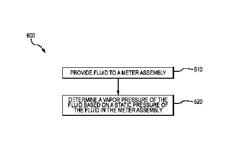
FIG. 6 shows a method 600 of determining a vapor pressure of a fluid. As shown
in FIG. 6, the method 600, in step 610, provides a fluid to a meter assembly,
such as, for
example, the meter assembly 10 described above with reference to FIG. 1. In
step 620,
the method 600 determines a vapor pressure of the fluid based on a static
pressure of the
fluid in the meter assembly.
During the step 610, fluid may be provided to the meter assembly 10 via, for
example, a branch on a pipeline, such as the system 500 shown in FIG. 5. As
shown in
FIG. 5, the branch is a loop that returns the fluid to the pipeline 501.
Alternatively, the
fluid may be provided to the meter assembly 10 via a non-returning branch. For
example, a fork from the pipeline 501 shown in FIG. 5 may empty into a
reservoir or
.. tank rather than return to the pipeline 501. The fluid may or may not
include vapor or
gas.
Step 620 may determine the vapor pressure of the fluid by, for example,
varying
the total or static pressure of the fluid in the meter assembly 10 until a
fluid phase
change is detected. For example, the static pressure of the fluid may be
increased until
vapor is no longer detected. Conversely, the static pressure may be decreased
until vapor
is detected. The fluid phase change may be detected by any suitable means,
such as, for
example, based on the sensor signals, such as detecting a change in a drive
gain or drive
signal as discussed above with reference to FIG. 3.
When the fluid phase change is detected, such as when a change in the drive
gain
is detected, the vibratory meter 5, or electronics coupled to the vibratory
meter 5, may
determine the pressure at the inlet and/or outlet of the meter assembly 10.
For example,
with reference to FIG. 5, the inlet pressure sensor 520 may measure the static
pressure
of the fluid at the inlet of the meter assembly 10 and the outlet pressure
sensor 530 may
measure the static pressure of the fluid at the outlet of the meter assembly
10.
Accordingly, the inlet static pressure and/or the outlet static pressure may
be associated
with the fluid phase change.
21
CA 03135823 2021-10-01
WO 2020/204919
PCT/US2019/025533
The inlet static pressure and the outlet static pressure can be used in
equation [7]
above to determine a static pressure in the meter assembly. For example, the
outlet
pressure may be P1, and P2 may be a pressure of the fluid in the meter
assembly. The
height related terms, pgzi and pgz2 may be used to account for change in
height of the
fluid in the meter assembly due to, for example, conduit geometry. For
example, bow
shaped conduits, such as those of the meter assembly 10 described above, may
have an
elevation change. The dynamic velocity terms 4, 4 may similarly be solved for
by
measuring a density and a flow rate of the fluid and knowing the dimensions of
the
conduits and the pipe coupled to the conduits' inlets and outlets. Similarly,
the viscous
pv2 fL
pressure drop term, ¨ --, may also be determined.
2 D
Accordingly, the method 600 may determine the vapor pressure of the fluid in
the meter assembly 10 based on a detection of a vapor. That is, the static
pressure may
be varied until the phase change is detected and the associated static
pressure may then
be determined based on, for example, the outlet pressure. The static pressure
may
therefore be the vapor pressure. As can be appreciated, the change in the
pressure in the
meter assembly may be based on a cross-sectional area change in the meter
assembly.
The above describes the vibratory meter 5, in particular the meter electronics
20,
and a method 600 that determine a vapor pressure of the fluid in the meter
assembly 10
based on a static pressure of the fluid in the meter assembly 10. Because the
static
pressure is of the fluid in the meter assembly 10, rather than a static
pressure of the fluid
in, for example, a pipeline in which the meter assembly is inserted, the
determined vapor
pressure may be more accurate. As a result, the operation of the vibratory
meter 5 and
the meter electronics 20 is improved because the values provided by the
vibratory meter
5 and meter electronics 20 are more accurate. More accurate measurements in
the
technical field of vapor pressure measurements can improve other technical
fields, such
as fluid process controls, or the like.
The detailed descriptions of the above embodiments are not exhaustive
descriptions of all embodiments contemplated by the inventors to be within the
scope of
the present description. Indeed, persons skilled in the art will recognize
that certain
elements of the above-described embodiments may variously be combined or
eliminated
to create further embodiments, and such further embodiments fall within the
scope and
22
CA 03135823 2021-10-01
WO 2020/204919
PCT/US2019/025533
teachings of the present description. It will also be apparent to those of
ordinary skill in
the art that the above-described embodiments may be combined in whole or in
part to
create additional embodiments within the scope and teachings of the present
description.
Thus, although specific embodiments are described herein for illustrative
purposes, various equivalent modifications are possible within the scope of
the present
description, as those skilled in the relevant art will recognize. The
teachings provided
herein can be applied to other methods, apparatus, electronics, systems, or
the like, for
determining a vapor pressure of a fluid and not just to the embodiments
described above
and shown in the accompanying figures. Accordingly, the scope of the
embodiments
described above should be determined from the following claims.
23