Note: Descriptions are shown in the official language in which they were submitted.
1
TITLE OF THE INVENTION
Method and system for real-time wide-field dynamic temperature sensing
FIELD OF THE INVENTION
[0001] The present invention relates to temperature sensing. More
specifically, the present invention is
concerned with a method and system for fast wide-field upconversion
luminescence lifetime thermometry.
BACKGROUND OF THE INVENTION
[0002] Temperature is an important parameter associated with a number of
physical, chemical, and
biological processes. Accurate and real-time, temperature sensing at
microscopic scales is essential to both
industrial applications and scientific research, including the examination of
internal strains in turbine blades, control of
the synthesis of ionic liquids, and theranostics of cancer.
[0003] Phosphorescence lifetime imaging (PLI) has emerged as a promising
approach to temperature
sensing, due to its high spatial resolution, high temperature sensitivity, and
resilience to experimental perturbation.
Because phosphorescence can be both excited and detected optically, the
resulting non-contact phosphorescence
lifetime imaging possesses a high spatial resolution. This advantage not only
overcomes the intrinsic limitation in
spatial resolution of imaging thermography due to the long wavelengths of
thermal radiation but also avoids heat-
transfer-induced inaccuracy in conventional contact methods. Moreover,
independent of accurate prior knowledge of
the physical properties of the sample, in terms of emissivity and Griineisen
coefficient, phosphorescence lifetime
imaging brings in higher flexibility in sample selection. Furthermore,
phosphorescence lifetime imaging is less
susceptible than intensity-based measurements to inhomogeneous signal
attenuation, stray light, photobleaching,
light path length, and excitation intensity variations. Finally,
phosphorescence lifetime imaging does not rely on the
concentration of labeling agents, which eliminates the need for special
ratiometric probes.
[0004] Phosphorescence lifetime imaging (PLI) in temperature mapping
depends on temperature indicators
and optical imaging instruments.
[0005] Recent advances in biochemistry, materials science, and molecular
biology have discovered numerous
labeling agents for phosphorescence lifetime imaging-based temperature
sensing, such as lanthanide-doped
upconverting nanopartides (UCNPs) for example. Leveraging the long-lived
excited states provided by the lanthanide
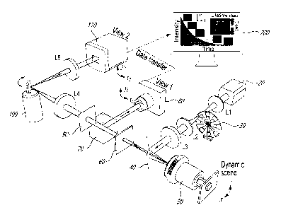
ions, upconverting nanopartides can sequentially absorb two, or more, low-
energy near-infrared photons and convert
Date Regue/Date Received 2022-08-23
2
them to one higher-energy photon, in an upconversion process allowing using
excitation power densities several orders
of magnitude lower than those needed for simultaneous multiphoton absorption.
The near-infrared excitation, with smaller
extinction coefficients, also gains deeper penetration. Besides, the
upconverted luminescence, particularly the
Boltzmann-coupled emission bands in co-doped erbium/ytterbium (Er-3-EYb-3)
systems, is highly sensitive to temperature
changes. Moreover, long-lived emission, in the range between microseconds and
milliseconds, of upconverting
nanopartides circumvents interferences from autofluorescence and scattering
during image acquisition, which translates
into improved imaging contrast and detection sensitivity. Finally, because of
advances in their synthesis and surface
functionalization coupled with the innovation of core/shell engineering,
upconverting nanopartides have become much
brighter, photostable, biocompatible, and non-toxic. As a result, upconverting
nanoparticles are one of the
frontrunners in temperature indicators for phosphorescence lifetime imaging.
[0006] Advanced optical imaging is the other indispensable constituent
in phosphorescence lifetime
imaging (PLI)-based temperature mapping. Phosphorescence lifetime imaging
(PLI) typically uses scanning time-
correlated single-photon counting (TCSPC) to determine phosphorescence decay
point by point. To accelerate data
acquisition, wide-field methods comprise parallel collection in the time-
domain and frequency-domain; In the time-
domain, these methods extend time-correlated single-photon counting (TCSPC) to
wide-field imaging.
Photoluminescence decay over a 2D field of view (FOV) is synthesized from
above 100,000 frames. Alternatively,
frequency-domain wide-field phosphorescence lifetime imaging methods use phase
difference between the intensity-
modulated excitation and the received phosphorescence signal to determine the
2D lifetime distribution.
[0007] Although allowing high signal-to-noise ratios, scanning
operation in time-correlated single-
photon counting (TCSPC) leads to an excessively long imaging time to form a
two-dimensional (2D) lifetime map
because extended pixel dwell time is required to record the long-lived
phosphorescence. Wide-field
phosphorescence lifetime imaging (PLI) in the time domain require the
phosphorescence emission to be precisely
repeatable, which is not practical in real measurement. In frequency-domain
wide-field phosphorescence lifetime
imaging, limited by the range of frequency synthesizers, the measurable
lifetimes are mostly restricted to below 100
ils, which is shorter than the lifetimes of most upconverting nanoparticles
(UCNPs). Akin to the time-domain
systems, frequency-domain systems rely on the integration over many periods of
modulation intensity, during which
the samples must remain stationary. Thus far, existing phosphorescence
lifetime imaging methods fall short in high-
resolution 2D temperature sensing of moving samples.
[0008] Despite remarkable advances in luminescent temperature
indicators, optical instruments still
Date Regue/Date Received 2022-08-23
3
lack the ability of wide-field phosphorescence lifetime imaging in real time,
thus falling short in dynamics temperature
mapping.
[0009] There is still a need in the art for a system and a method for
imaging thermometry for real-time
wide-field dynamic temperature sensing.
SUMMARY OF THE INVENTION
[0010] More specifically, in accordance with the present invention, there
is provided a method for real-time
wide-field dynamic temperature sensing of an object, comprising producing wide-
field illumination to upconverting
nanopartides at the object plane, collecting a light emitted by the
upconverting nanoparticles, dividing a collected
light into a reflected component and a transmitted component; imaging the
reflected component into a first image,
imaging the transmitted component into a second image; processing the images;
and reconstruction of the object
from resulting proceed images.
[0011] There is further provided a system for real-time wide-field
dynamic temperature sensing of an
object, comprising an illumination unit configured to produce wide-field
illumination to upconverting nanoparticles at
the object plane; an objective collecting light emitted by the upconverting
nanopartides; a beam splitter dividing a
collected light into a reflected component and a transmitted component; a
spatiotemporal integrator imaging the
reflected component into a first image; a spatial encoder encoding the object
into spatially encoded frames, a rotating
mirror temporally shearing resulting spatially encoded, and a camera
spatiotemporally integrating a resulting spatially
encoded and temporally sheared object into a second image; and a processing
unit reconstructing the object from
the first and the second images.
[0012] Other objects, advantages and features of the present invention
will become more apparent upon
reading of the following non-restrictive description of specific embodiments
thereof, given by way of example only
with reference to the accompanying drawings.
BRIEF DESCRIPTION OF THE DRAWINGS
[0013] In the appended drawings:
[0014] FIG. 1 is a schematic view of a system according to an embodiment
of an aspect of the present
disclosure;
Date Regue/Date Received 2022-08-23
4
[0015] FIG. 2A shows images of core/shell upconverting nanoparticles
acquired with a transmission electron
microscope; scale bar: 25 nm;
[0016] FIG. 2B shows normalized upconversion spectra of upconverting
nanoparticles shown in FIG. 2A;
[0017] FIG. 2C shows simplified energy level diagram of Yb3+-Er3+ energy
transfer upconversion excitation and
emission;
[0018] FIG. 2D shows temporally projected image of phosphorescence
intensity decay of the 5.6-nm-thick-shell
upconverting nanopartid es covered by a negative resolution target;
[0019] FIG. 2E shows a comparison of averaged light fiuence distribution
along the horizontal bars (I) and vertical
bars (II) of Element 5 in Group 4 on the resolution target; error bar standard
deviation;
[0020] FIG. 2F shows lifetime maps of upconverting nanopartides with the
shell thicknesses of 1.9 nm, 3.5 nm, and
5.6 nm covered by transparencies of letters "C", "A", and "N" in green
emission;
[0021] FIG. 2G shows time-lapse averaged phosphorescence emission
intensities of the samples;
[0022] FIG. 2H shows histograms of phosphorescence lifetimes in the
letters shown in FIG. 2F;
[0023] FIGs. 3A-3B show lifetime images of green (a) and red (b)
upconversion emission bands under
different temperatures;
[0024] FIGs. 3C-3D show normalized phosphorescence decay curves of green
(FIG. 3C) and red (FIG. 3D)
emission bands at different temperatures, averaged over the entire field of
view;
[0025] FIG. 3E shows the relationship between temperature and mean
lifetimes of green and red emissions
with linear fitting, error bar indicating standard deviation from three
independent measurements;
[0026] FIG. 3F shows the normalized contrast versus tissue thickness for
green and red emission bands fitted
by using the Beer's law;
[0027] FIG. 3G shows longitudinal temperature monitoring of a phantom
covered by 0.5 mm-thick chicken
tissue;
[0028] FIG. 4A shows representative time-integrated images of a moving
onion epidermis cell sample
Date Recue/Date Received 2022-08-23
5
labeled by upconverting nanopartides;
[0029] FIG. 4B shows phosphorescence lifetime images corresponding to
FIG. 4A;
[0030]
FIG. 4C shows phosphorescence decay at four selected areas, marked by the
solid boxes in the
first panel of FIG. 4A, with different intensities;
[0031]
FIG. 4D shows time histories of averaged fluence and corresponding
temperature in four selected
regions during translational motion of the sample;
[0032]
FIGs. 5 show image registration in dual-view data acquisition by single-shot
photoluminescence
lifetime imaging thermometry (SPLIT): FIG. 5A shows an image acquired in View
1; FIG. 5B shows an image
acquired in View 2 without using optical shearing; FIG. 5C shows a co-
registered image in View 1;
[0033]
FIGs. 6 show simulations of dual-view plug-and-play alternating direction
method of multipliers
(PnP-ADMM) reconstruction: FIG. 6A shows a comparison of representative frames
of the reconstructed result with
the ground truth; FIG. 6B shows a comparison of three local features in Frame
1 of the reconstructed result with the
ground truth, marked by the red-= round-dotted line, magenta= square-dotted
line, and black-dashed lines boxes;
FIG. 6C shows normalized averaged intensity of the reconstructed result versus
the frame index, the error bar
representing standard deviation;
[0034]
FIG. 7 shows X-ray powder diffraction patterns of upconverting nanoparticles
(UCNPs), the core-
only and core/shell NaGdF4:Er3+, Yb3-E/NaGdF4 upconverting nanopartides
(UCNPs) following their growth by
increasing the shell thickness; red dotted lines showing diffraction peaks of
pure hexagonal NaGdF4;
[0035]
FIGs. 8 show characterization sensitivity of the single-shot
photoluminescence lifetime imaging
thermometry (SPLIT): FIG. 8A shows temporally integrated reconstructed image
at the excitation laser power density
of 0.06 W/mm2; FIG. 8B shows the normalized intensity as a function of time
with a fitting curve;
[0036]
FIG. 9 shows a measurement of the green upconversion emission lifetime of
the 5.6 nm-thick-
shell upconverting nanoparticles (UCNPs) using time-correlated single-photon
counting (TCSPC);
Date Regue/Date Received 2022-08-23
6
[0037] FIGs. 10 show comparison of quality of images reconstructed by
using different algorithms:
FIG. 10A shows letter "C" reconstructed by using the single-view two-step
iterative thresholding/shrinkage (TwIST)
method, dual-view two-step iterative thresholding/shrinkage (TwIST) method,
and dual-view plug-and-play alternating
direction method of multipliers (PnP-ADMM) method, respectively; FIG. 10B ad
FIG. 10, like FIG. 10A, for letters "A"
and "N"; FIG. 10D shows a comparison of the selected line profiles of the
reconstructed images of letter "C"; FIG.
10E and FIG. 10GF, like FIG. 10D for letters "A" and "N". FIG. 10G, FIG. 10H
and FIG. 101 show lifetime maps of the
three letters produced by the single-view two-step iterative
thresholding/shrinkage (TwIST) method, showing single-
view plug-and-play alternating direction method of multipliers (PnP-ADMM) in
FIG. 10H, and plug-and-play
alternating direction method of multipliers (PnP-ADMM) in FIG. 101; insets
showing zoom-in views of three local
areas;
[0038] FIG. 11 shows quantification of relative temperature
sensitivities of green and red upconversion
emissions of the core/shell NaGdF4:Er3+, Yb3+/NaGdF4 upconverting
nanoparticles (UCNPs) with a 5.6 nm-thick shell.
Error bar: standard deviation;
[0039] FIGs. 12 show quantification of single-shot photoluminescence
lifetime imaging thermometry
(SPLIT)'s imaging depth: FIG. 12A shows experimental system; FIG. 12 B shows
temporally projected images of the
reconstructed dynamic scene at the depth from 0 to 1 mm with green emission;
FIG. 12c shows same as FIG. 12B
for red emission; FIG. 12A shows comparison of normalized intensity of a
representative cross-section, marked by
the dashed line in the first panel in FIG. 12B, for various imaging depths;
FIG. 12E same as FIG. 12D for red
emission, the representative cross-section being marked by the dashed line in
the first panel in FIG. 12C;
[0040] FIGs. 13 show longitudinal temperature monitoring using green
in FIG. 13A and red in FIG. 13B
luminescence emissions from the 5.6 nm-thick upconverting nanopartides (UCNPs)
covered by a transmissive mask
of letters "rob";
[0041] FIGs. 14 shows demonstration of single-shot photoluminescence
lifetime imaging thermometry
(SPLIT) with a fresh beef tissue phantom: FIG. 14A shows sample preparation;
FIG. 14 B shows temporally
projected images of the reconstructed dynamic scene at the depth from 0.09 to
0.60 mm with green emission; FIG.
14C shows same as FIG. 14B for red emission; FIG. 14D shows cross-sections of
a selected spatial feature, marked
by the solid line in FIG. 14B, for various depths; FIG. 14E shows same as FIG.
14D for red emission; FIG. 14F shows
Date Regue/Date Received 2022-08-23
7
normalized fluence versus tissue thickness for green and red emission fitted
using Beer's law; FIG. 14G shows
lifetimes as the function of the thickness for green emission (circles; the
mean value being plotted in solid line) and
red emission (diamonds; the mean value being plotted as the dashed line), the
error bar corresponding to standard
deviation, the right insets showing the decay of normalized average intensity
at the depth of 0.09 mm for green and
red emissions;
[0042] FIGs. 15 show single-layer onion cell sample: FIG. 15 A shows
an image of the sample taken
by a bright field microscope; FIG. 15B shows a confocal microscopy of green
upconversion emission of upconverting
nanopartides (UCNPs) diffused in an individual onion cell, marked by the
dashed box in FIG. 15A;
[0043] FIGs. 16 show schematics of an optoelectronic streak camera
(FIG. 16A) and a mechanical
streak camera (FIG. 16B) in their conventional operations;
[0044] FIGs. 17 show comparison between line-scanning microscopy and
single-shot
photoluminescence lifetime imaging thermometry (SPLIT) in 2D photoluminescence
lifetime imaging (PLI) capability:
Fig. 17A shows a experimental system of line-scanning microscopy, the moving
upconverting nanoparticles (UCNPs)
sample beings loaded onto a translation stage, the moving directions being
marked by arrows: FIG. 17B shows one-
dimensional photoluminescence lifetime imaging (PLI) by using the line-
scanning system; FIG. 17C shows a 2D
temperature map synthesized by using the data in FIG. 17B; FIG. 17D shows
seven 2D lifetime maps of the sample
moving along vertical direction captured by using the single-shot
photoluminescence lifetime imaging thermometry
(SPLIT);
[0045] FIGs. 18 shows a comparison between the thermal imaging camera
and single-shot
photoluminescence lifetime imaging thermometry (SPLIT) in temperature imaging:
FIGs. 18A-and 18B show
experimental system using thermal imaging camera (FIG. 18A) or
photoluminescence lifetime imaging thermometry
system (FIG. 18B), the sample and mask being heated up by a blackbody
radiator.; FIG. 18C shows a temperature
image captured by using the thermal imaging camera; FIG. 18D shows as FIG. 18C
using single-shot
photoluminescence lifetime imaging thermometry (SPLIT); FIG. 18E and FIG. 18
show selected line profile from FIG.
18C and FIG. 18D, respectively; FIG. 18G shows same as FIG. 18A using a
translation stage to move the mask with
the room temperature; FIG. 18H shows a temperature image captured by the
system in FIG. 18; FIG. 181 shows as
elected line profile from FIG. 18H; and
Date Regue/Date Received 2022-08-23
8
[0046]
FIG. 19 is an iillustration of the principle of single-shot
photoluminescence lifetime imaging
thermometry (SPLIT).
DESCRIPTION OF ILLUSTRATIVE EMBODIMENTS
[0047] The present invention is illustrated in further details by the
following non-limiting examples.
[0048]
A system according to an embodiment of an aspect of the present disclosure
is illustrated for
example in FIG. I.
[0049]
A laser beam from a laser source 20 passes through an expander consisting of
a first 4f system
consisting of lenses L1 and L2 (focal length 50-mm, singlet). A chopper 30 is
placed at the back focal plane of the
first lens L1 of 4f system to generate 50- ps optical pulses. Then, the pulses
pass through a 100-mm focal length
lens L3 and is reflected by a dichroic mirror 40 to generate a focus on the
back focal plane of an objective lens 50
with a field of view of at least 1.5 mm x 1.5 mm.
[0050]
The laser source 20 may be a 980-nm continuous-wave laser or a 980-mm pulse
laser. The
expander may be an optical beam expander. The chopper 30 may be an optical
chopper or an electro-optic
modulator or an acoustic optical modulator. The dichroic mirror 40 may be a
short-pass filter with a cut off
wavelength of 750 nm.
[0051]
This illumination configuration, using a 4f system to expand the diameter of
the laser beam,
produces wide-field illumination, with a 1.5x1.5 mm2 field of view, to
upconverting nanoparticles at the object plane.
[0052]
The near-infrared excited upconverting nanoparticles emit upconverted
phosphorescence light in the
visible spectrum. The decay of light intensity over the 2D field of view is a
dynamic scene 1(x,y,t). The emitted light is
collected by the objective lens 50, transmitted through the dichroic mirror
40, and is filtered by a band-pass filter 60.
A beam splitter 70 then equally divides the light into a reflected and a
transmitted components.
[0053]
The reflected component is imaged by a complementary metal oxide
semiconductor (CMOS)
camera via spatiotemporal integration (operator T) as View 1, with optical
energy distribution El (x1.36). Alternatively,
charge-coupled device (CCD) cameras, scientific complementary metal oxide
semiconductor (sCMOS) cameras, or
electron-multiplying charged-coupled device (EMCCD) cameras may be used.
Date Regue/Date Received 2022-08-23
9
[0054] The transmitted component forms an image, using front optics
such as a camera lens, an
objective lens, and a telescope for imaging to an intermediate image plane,
the dynamic scene on a transmissive
encoding mask 90 with a pseudo-random binary pattern (Fineline Imaging, 50%
transmission ratio; 60-pm encoding
pixel size) (operator C). Alternatively, a spatial light modulator such as a
digital micro-mirror device, or a printed mask
loaded on a translation stage may be used. Then, the spatially encoded scene
in the intermediate image plane is
relayed by relay optics, such as by a second 4f imaging system (100-mm focal
length lenses L4 and L5) as
illustrated, or by a tube lens system, to the sensor plane of an electron-
multiplying charged-coupled device (EMCCD)
camera 110 for View 2 imaging. A global shutter scientific complementary metal
oxide semiconductor (sCMOS)
camera may also be used.
[0055] A galvanometer scanner 100, placed at the Fourier plane of the
4f imaging system, temporally
shears (operator S) the spatially encoded frames linearly to different spatial
locations along the x-axis of the electron-
multiplying charged-coupled device (EMCCD) camera 110 according to their time
of arrival. Other rotating mirror
such as a polygonal scanner or a resonant scanners, may be used. Finally, the
spatially encoded and temporally
sheared dynamic scene is recorded by the electron-multiplying charged-coupled
device (EMCCD) camera 110 via
spatiotemporal integration, as View 2, with optical energy distribution E2
(X2.3/2).
[0056] Both images are transferred to a processing unit 200 and used
for reconstruction of the object.
The system may be described in a forward model as follows:
[0057] E = TM /(x-õy.t), (1)
where E is the concatenation of measurements [Er, ezEr,]T, M is a linear
operator 11, (-4SC] 7, and a is a scalar factor
introduced to balance the energy ratio between the two views View 1 and View 2
during measurement. After data
acquisition, E is obtained by retrieving the datacube of the dynamic scene by
leveraging the spatiotemporal sparsity
of the dynamic scene and the prior knowledge of each operator. Based on the
plug-and-play alternating direction
method of multipliers (PnP-ADMM), reconstruction is achieved by solving the
following minimization problem:
f1
[0058]
= argatiiint¨ ¨ EHE RCIr) + 1+0)1.
2
[0059] m .1i represents the 1, norm,
IrMt - Eli'. is a fidelity term representing the similarity
Date Regue/Date Received 2022-08-23
10
between the measurement and the estimated result. R(.) is the implicit
regularizer that promotes sparsity in the
dynamic scene. I+ (=) represents a non-negative intensity constraint
[0060]
Plug-and-play alternating direction method of multipliers (PnP-ADMM)
implements a variable
splitting strategy with a state-of-the-art denoiser to obtain fast and closed-
form solutions to each sub-optimization
problem, which produces a high image quality in reconstruction. The retrieved
datacube of the dynamic scene has a
sequence depth, defined as the number of frames in a reconstructed movie, of
12-100 frames, each containing 460
x 460 (X,) pixels. The imaging speed is tunable from 4 to 33 thousand frames
per second (kfps).
[0061]
The reconstructed datacube is then converted to a photoluminescence lifetime
map. In
particular, for each (x,y) point, the area under the normalized intensity
decay curve is integrated to report the value
of the photoluminescence lifetime. Finally, using the approximately linear
relationship between the lifetime of the
upconverting nanopartides (UCNPs) and the physiologically relevant temperature
range, between 20 and 46 C in the
present experiment, the 2D temperature distribution, T(x, y), is calculated as
follows:
y,t)
riCw.y) = ct 0)
(3)
SA ICr,Y,
[0062]
ct is a constant, and; is the absolute temperature sensitivity. Leveraging
the intrinsic frame rate
of the charged-coupled device (EMCCD) camera 110, the system can generate
lifetime-determined temperature
maps at a video rate of 20 Hz.
[0063]
FIG. 2A shows images of core/shell upconverting nanoparticles acquired Adh a
transmission electron
microscope. FIG. 2B shows normalized upconversion spectra of upconverting
nanopartides shown in FIG. 2A. FIG. 2C shows
simplified energy level diagram of Yb3+-Er3+ energy transfer upconversion
excitation and emission. FIG. 2D shows temporally
projected image of phosphorescence intensity decay of the 5.6-nm-thick-shell
upconverting nanopartides covered by a
negative resolution target. FIG. 2E shows a comparison of averaged light
fluence distribution along the horizontal bars (I) and
vertical bars (II) of Element 5 in Group 4 on the resolution target. FIG. 2F
shows lifetime maps of upconverting nanoparticles
with the shell thicknesses of 1.9 nm, 3.5 nm, and 5.6 nm covered by
transparencies of letters "C", "A", and "N" in green emission.
FIG. 2G shows time-lapse averaged phosphorescence emission intensities of the
samples. FIG. 2H shows histograms of
phosphorescence lifetimes in the letters shown in FIG. 2F.
Date Regue/Date Received 2022-08-23
11
[0064] FIGs. 3 show single-shot temperature mapping using single-shot
photoluminescence lifetime imaging
thermometry (SPLIT). FIGs. 3A-3B show lifetime images of green (A) and red (
B) upconversion emission bands under
different temperatures. FIGs. 3C-3D show normalized phosphorescence decay
curves of green (C) and red (D) emission
bands at different temperatures, averaged over the entire field of view. FIG.
3E shows the relationship between
temperature and mean lifetimes of green and red emissions with linear fitting.
FIG. 3F shows the normalized contrast
versus tissue thickness for green and red emission bands with single-component
exponential fitting. FIG. 3G shows
longitudinal temperature monitoring of a phantom covered by 0.5 mm-thick
chicken tissue.
[0065] FIGs. 4 show dynamic single-cell temperature mapping. FIG. 4A
shows representative time-
integrated images of a moving onion epidermis cell sample labeled by
upconverting nanoparticles. FIG. 4B shows
phosphorescence lifetime images corresponding to FIG. 4A. FIG. 4C shows
phosphorescence decay at four selected
areas, marked by the solid boxes in the first panel of FIG. 4A, varied
intensities. FIG. 4D shows time histories of
averaged fluence and corresponding temperature in the four selected regions
during the sample's translational
motion.
[0066] The present optical temperature mapping method synergistically
combines dual-view optical streak
imaging with compressed sensing, to record wide-field luminescence decay of
Er3 , Yb3+ co-doped NaGdF4
upconverting nanoparticles in real time, from which a lifetime-based 2D
temperature map is obtained in a single
exposure. The method enables high-resolution longitudinal temperature
monitoring beneath a thin scattering medium
and dynamic temperature tracking of a moving biological sample at single-cell
resolution.
[0067] Thus a method according to an aspect of the present disclosure
comprises producing wide-field
illumination to upconverting nanoparticles at the object plane, by expanding
the laser beam diameter, using a 4f
system or an optical beam expander for example. The near-infrared excited
upconverting nanoparticles emit
upconverted phosphorescence light in the visible spectrum. The decay of the
emitted light intensity over the 2D field of
view is a dynamic scene 1(x,y,t). The emitted light is collected and equally
divided into a reflected component and a
transmitted component. The method then comprises imaging the reflected
component (View 1) by spatiotemporal
integration using a complementary metal oxide semiconductor (CMOS) camera, a
charge-coupled device (CCD)
camera, a scientific complementary metal oxide semiconductor (sCMOS) camera,
or an electron-multiplying
charged-coupled device (EMCCD) camera for example, and imaging the transmitted
component (View 2) by spatial
encoding using a printed mask or a spatial light modulator such as a digital
micro-mirror device, or a printed mask
loaded on a translation stage, temporal shearing, using a rotating mirror such
as a galvanometer scanner, a
polygonal scanner or a resonant scanner for example, and spatiotemporal
integration, using a highly sensitive
Date Regue/Date Received 2022-08-23
12
cameras such as an electron-multiplying charged-coupled device (EMCCD) or a
global shutter scientific
complementary metal oxide semiconductor (sCMOS) for example. The data of the
images are processed for
denoising, cropping, and calibration of the obtained two views, and video
reconstruction or compressed sensing
based video reconstruction is performed.
[0068] In the present single-shot phosphorescence lifetime imaging
thermometry method, high parallelism
in the data acquisition improves the overall light throughput. The method,
comprising single-shot temperature
sensing over a 2D field of view, allows improved measurement accuracy by
avoiding scanning motion artifacts and
laser intensity fluctuation. The present single-shot phosphorescence lifetime
imaging thermometry method and
system extend the application scope of phosphorescence lifetime imaging to
observing non-repeatable temperature
dynamics. They allow high tunability of imaging speeds, which accommodates a
variety of upconverting nanoparticles
with a wide lifetime span.
[0069] From the perspective of system design, both the dual-view data
acquisition and the plug-and-play
alternating direction method of multipliers (PnP-ADMM) method support high
imaging quality in the present single-
shot phosphorescence lifetime imaging thermometry system and method. In
particular, View 1 preserves the spatial
information in the dynamic scene. Meanwhile, View 2 retains temporal
information by optical streaking via time-to-
space conversion. Altogether, both views maximally keep rich spatiotemporal
information. In software, the plug-and-
play alternating direction method of multipliers (PnP-ADMM) method provides a
powerful modular structure, which
allows separated optimization of individual sub-optimization problems with an
advanced denoising algorithm to
generate high-quality image restoration results.
[0070] The present single-shot phosphorescence lifetime imaging
thermometry method and system
provide a versatile temperature-sensing platform. In materials
characterization, they may be used in the stress
analysis of metal fatigue in turbine blades. In biomedicine, they may be
implemented for accurate sub-cutaneous
temperature monitoring for theranostics of skin diseases such as melanoma. The
microscopic temperature mapping
ability may also be exploited for the studies of temperature-regulated
cellular signaling. Finally, the operation of the
method and system may be extended to Stokes emission in rare-earth
nanoparticles and spectrally resolved
temperature mapping.
[0071] More details are discussed hereinbelow, presenting the optical
temperature mapping system and
method according to embodiments of the present disclosure, referred to as
single-shot photoluminescence lifetime
imaging thermometry (SPLIT). Synergistically combining dual-view optical
streak imaging with compressed sensing,
Date Regue/Date Received 2022-08-23
13
single-shot photoluminescence lifetime imaging thermometry (SPLIT) records
wide-field luminescence decay of Er3+,
Yb3+ co-doped NaGdF4 Upconverting nanoparticles (UCNPs) in real time, from
which a lifetime-based 2D
temperature map is obtained in a single exposure. Thus single-shot
photoluminescence lifetime imaging thermometry
(SPLIT) enables longitudinal 2D temperature monitoring beneath a thin
scattering medium and dynamic temperature
tracking of a moving biological sample at single-cell resolution.
[0072] A single-shot photoluminescence lifetime imaging thermometry
(SPLIT) system according to an
embodiment of an aspect of the present invention is shown in FIG. 1, showing
data acquisition and image
reconstruction of luminescence intensity decay in a letter "C". As described
hereinabove, a 980-nm continuous-wave
laser (BWT, DS3-11312-113-LD) is used as the light source. The laser beam
passes through a 4f system consisting
of two 50-mm focal length lenses (L1 and L2, Thorlabs, LA1255). An optical
chopper (Scitec Instruments, 300CD) is
placed at the back focal plane of lens L1 to generate 50-ps optical pulses.
Then, the pulse passes through a 100-mm
focal length lens (L3, Thorlabs, AC254-100-B) and is reflected by a short-pass
dichroic mirror (Edmund Optics, 69-
219) to generate a focus on the back focal plane of an objective lens (Nikon,
CF Achro 4x). This illumination scheme
produces wide-field illumination (1.5x1.5 mm2 field of view (FOV)) to
Upconverting nanoparticles (UCNPs) at the
object plane.
[0073] The near-infrared excited Upconverting nanoparticles (UCNPs)
emit light in the visible spectral
range. The decay of light intensity over the 2D field of view (FOV) is a
dynamic scene, denoted by i(x., y, t). The
emitted light is collected by the same objective lens, transmits through the
dichroic mirror, and is filtered by a band-
pass filter (Thorlabs, MF542-20 or Semrock, FF01-660/30-25). Then, a beam
splitter (Thorlabs, B5013) equally
divides the light into two components. The reflected component is imaged by a
complementary metal oxide
semiconductor (CMOS) camera (FLIR, G53-U3-2356M-C) with a camera lens
(Fujinon, HF75SA1) via
spatiotemporal integration (denoted as the operator T) as View 1, whose
optical energy distribution is denoted by
(x1,71)=
[0074] The transmitted component forms an image of the dynamic scene on
a transmissive encoding
mask with a pseudo-random binary pattern (Fineline Imaging, 50% transmission
ratio; 60-pm encoding pixel size).
This process of spatial encoding is denoted by the operator C. Then, the
spatially encoded scene is relayed to the
sensor plane of an electron-multiplying (EM) CCD camera (Nava Cameras, HNO
1024) by another 4f imaging
system consisting of two 100-mm focal length lenses (L4 and L5, Thorlabs,
AC254-100-A). A galvanometer scanner
(Cambridge Technology, 6220H), placed at the Fourier plane of the 4f imaging
system, temporally shears the
Date Regue/Date Received 2022-08-23
14
spatially encoded frames linearly to different spatial locations along the xõ-
axis of the electron-multiplying charged-
coupled device (EMCCD) camera according to their time of arrival. This process
of temporal shearing is denoted by
the operator S. Finally, the spatially encoded and temporally sheared dynamic
scene is recorded by the EMCCD via
spatiotemporal integration to form View 2, whose optical energy distribution
is denoted by a ("x2,y2).
[0075]
By combining the image formation of i(x10,1) and E(xõ, yõ), the data
acquisition of
single-shot photoluminescence lifetime imaging thermometry (SPLIT) is
expressed as follows:
E 'TP4 (1)
[0076]
E' denotes the concatenation of measurements LE,, aE,JT , M denotes the
linear operator
[1, aSC]T, and et is a scalar factor introduced to balance the energy ratio
between the two views during
measurement. The hardware of the single-shot photoluminescence lifetime
imaging thermometry (SPLIT) system is
synchronized for capturing both views (detailed in Methods) that are
calibrated before data acquisition (see
Supplementary Note 1 and FIG. 5).
[0077]
After data acquisition, E is processed an algorithm that retrieves the
datacube of the dynamic
scene by leveraging the spatiotemporal sparsity of the dynamic scene and the
prior knowledge of each operator.
Developed from the plug-and-play alternating direction method of multipliers
(PnP-ADMM) method, the
reconstruction algorithm of single-shot photoluminescence lifetime imaging
thermometry (SPLIT) solves the following
minimization problem:
I = arginin IITNIi ¨EH+R(i) 4(i)1 (2)
2
[0078]
represents the /2 norm. The fidelity term, -117Mi ¨ Ell, represents the
similarity
2
between the measurement and the estimated result. R() is the implicit
regularizer that promotes sparsity in the
dynamic scene. i 0 represents a non-negative intensity constraint. Compared to
existing reconstruction schemes,
the plug-and-play alternating direction method of multipliers (PnP-ADMM)
method implements a variable splitting
strategy with a state-of-the-art denoiser to obtain fast and closed-form
solutions to each sub-optimization problem,
which produces a high image quality in reconstruction (see FIG. 6 and
Supplementary Notes 2 and 3). The retrieved
datacube of the dynamic scene has a sequence depth, that is the number of
frames in a reconstructed movie, of
100 frames, each containing 460 x 460 (x,y) pixels. The imaging speed is
tunable from 4 to 33 thousand frames
Date Regue/Date Received 2022-08-23
15
per second (kfps).
[0079] A photoluminescence lifetime map is then generated by integrating
the area under the decay
curve 50. Finally, using the approximately linear relationship between the
UCNPs' lifetime and the physiologically
relevant temperature range (20-46 C in the present experiment), the 2D
temperature distribution, r(x,y), is
calculated as follows:
1 P Ocfry ,t)
nix,y) = ct+ (3)
Sa I y,
[0080] ct. is a constant, and .5 is the absolute temperature
sensitivity. The derivation of Relation 3 is
detailed in Supplementary Note 4 hereinbelow. Leveraging the intrinsic frame
rate of the electron-multiplying
charged-coupled device (EMCCD) camera, the photoluminescence lifetime imaging
thermometry (SPLIT) system
can generate lifetime-determined temperature maps at a video rate of 20 Hz.
[0081] For quantification of the system's performance of single-shot
photoluminescence lifetime
imaging thermometry (SPLIT), a series of core/shell upconverting nanoparticle
(UCNP) samples were prepared to
showcase the single-shot photoluminescence lifetime imaging thermometry
(SPLIT) imaging and temperature
sensing capabilities. These upconverting nanoparticles (UCNPs) shared the same
NaGdF4: 2 mol% Er3+, 20 mol%
Yb3+ active core of 14.6 nm in size, while differed by the thickness of their
undoped NaGdF4 passive shell of 1.9,
3.5, and 5.6 nm (FIG. 2A and Supplementary Note 5 hereinbelow). All of the
upconverting nanoparticles (UCNPs)
samples were of pure hexagonal crystal phase (FIGs. 7). Under the 980-nm
excitation, upconversion emission
bands of all samples were measured at around 525/545 and 660 nm, which
correspond to the 2H1112/45312 ¨> 4115/2
and 4F912 ¨> 4115/2 radiative transitions, respectively (FIGs. 2B-2C).
[0082] To characterize the spatial resolution of single-shot
photoluminescence lifetime imaging
thermometry (SPLIT), the 5.6 nm-thick-shell upconverting nanopartide (UCNP)
sample was covered with a negative
USAF resolution target (Edmund Optics, 55-622). Operating at 33 kfps, single-
shot photoluminescence lifetime
imaging thermometry (SPLIT) recorded the photoluminescence decay. The
temporally projected datacube reveals
that the intensity and contrast in the reconstructed image degrade with the
decreased spatial feature sizes,
eventually leading to the loss of structure whose size approaches that of the
encoding pixel (FIG. 2D). The spatial
resolution was thus determined to be 20 pm (FIG. 2E). Under these experimental
conditions, the minimum power
Date Regue/Date Received 2022-08-23
16
density for the single-shot photoluminescence lifetime imaging thermometry
(SPLIT) system was quantified to be
0.06 W/mm2(see Supplementary Note 6 hereinbelow and FIG. 8).
[0083] To demonstrate the ability of single-shot photoluminescence
lifetime imaging thermometry
(SPLIT) to distinguish different lifetimes, the Upconverting nanoparticles
(UCNPs) were imaged with shell
thicknesses of 1.9 nm, 3.5 nm, and 5.6 nm, covered by transparencies of
letters "C", "A", and "N", respectively,
using a single laser pulse. The lifetime maps of these samples are shown in
FIG. 2F, which reveals the averaged
lifetimes for the 4S3/2 excited state of samples "C", "A", and "N" to be 142
ps, 335 ps, and 478 ps, respectively
(FIGs. 2G-2H). These results were verified by using the standard time-
correlated single-photon counting (TCSPC)
method (see Supplementary Note 7 hereinbelow and FIG. 9).
[0084] Single-shot photoluminescence lifetime imaging thermometry
(SPLIT) reconstruction method is
thus shown to match existing mainstream algorithms popularly used in single-
shot compressed ultrafast imaging. By
using the experimental data, the comparison demonstrates that the dual-view
plug-and-play alternating direction
method of multipliers (PnP-ADMM) used by single-shot photoluminescence
lifetime imaging thermometry (SPLIT) is
more powerful in preserving spatial features while maintaining a low
background, which enables a more accurate
lifetime quantification and the ensuing temperature mapping (see Supplementary
Note 8 hereinbelow and FIG. 10).
[0085] For single-shot temperature mapping using single-shot
photoluminescence lifetime imaging
thermometry (SPLIT), the 5.6 nm-thick-shell upconverting nanoparticles (UCNPs)
was used as the temperature
indicator for single-shot photoluminescence lifetime imaging thermometry
(SPLIT). The temperature of the
upconverting nanoparticles (UCNPs) was controlled by a heating plate placed
behind the sample. To image the
green (4S3/2) and red (4F912) upconversion emissions, the sample was covered
by transparencies of a lily flower and
a maple leaf, respectively. The temperature of the entire sample was measured
with both a Type K thermocouple
(Omega, HH306A) and a thermal camera (FLIR, E4) as references. The
reconstructed lifetime images in the 20-
46 C temperature range are shown in FIGs. 3A, 3B. Plotted in FIGs. 3C, 3D, the
time-lapse averaged intensity over
the entire field of view (FOV) shows that the averaged lifetimes of green and
red emissions decrease from 489 to
440 ps and from 458 to 398 ps, which is due to their enhanced multiphonon
deactivation at higher temperatures.
The relationship between the temperatures and lifetimes for both emission
channels (FIG. 3E) was further plotted
Finally, the temperature sensitivities in the preset temperature range were
calculated to be 5 = ¨1.90 Rs /DC for
green emission and .5 = ¨2.40 itstt for red emission (see Supplementary Note 9
and FIG. 11). The higher
Date Regue/Date Received 2022-08-23
17
temperature sensitivity of the red-emitting state compared to the green state
results from the greater energy
separation from their respective lower-laying excited states. Since
multiphoton relaxation rate depends
exponentially on the number of phonons necessary to non-radioactively
deactivate a given excited state to the one
just below, the temperature-induced changes to the phonon energies (reducing
the number of required phonons for
quenching) will have a greater influence over the excited states with larger
energy gap between each other. These
results establish lifetime-temperature calibration curves (see Relation 3) for
ensuing thermometry experiments.
[0086] To demonstrate the feasibility of single-shot photoluminescence
lifetime imaging thermometry
(SPLIT) in a biological environment, longitudinal temperature monitoring under
a phantom, made by using the 5.6
nm-thick-shell upconverting nanoparticles (UCNPs) covered by lift-out grids
(Ted Pella, 460-2031-S), overlaid by
fresh chicken breast tissue, was performed. The imaging depth of single-shot
photoluminescence lifetime imaging
thermometry (SPLIT) was investigated with varied tissue thicknesses of up to 1
mm (FIG. 3F, FIG. 12,
Supplementary Note 10). The chicken tissue of 0.5 mm thickness, where both the
green and red emissions
produced images with full spatial features of the lift-out grid, was used in
the following imaging experiments.
Subsequently, the temperature of the sample was cycled between 20 C and 46
C. The lifetime distributions of both
green and red emissions and their corresponding temperature maps were
monitored every 20 minutes and 23
minutes, respectively, for about 4 hours (see the full evolution in FIG. 13).
As shown in FIG. 3G, the results are in
good agreement with the temperature change preset by the heating plate, and
decisively showcase how single-shot
photoluminescence lifetime imaging thermometry (SPLIT) can noninvasively map
2D temperatures over time with
high accuracy beneath biological tissue.
[0087] Single-shot photoluminescence lifetime imaging thermometry
(SPLIT) was also demonstrated
using a fresh beef phantom as a scattering medium, where both water and blood
are present (FIG. 14 and
Supplementary Note 10). The results reveal better penetration of red emission
over the green counterpart due to its
weaker scattering and absorption by blood. More importantly, the results
confirm the independence of the measured
photoluminescence lifetime of upconverting nanoparticles (UCNPs) to tissue
thickness and hence the excitation
light power density in the present example (0.4 W/mm2).
[0088] In tests of single-cell dynamic temperature tracking using single-
shot photoluminescence
lifetime imaging thermometry (SPLIT), to apply single-shot photoluminescence
lifetime imaging thermometry
(SPLIT) to dynamic single-cell temperature mapping, a single-layer onion
epidermis sample labeled by the 5.6 nm-
Date Regue/Date Received 2022-08-23
18
thick-shell upconverting nanoparticles (UCNPs) (Supplementary Note 11 and FIG.
15) was tested. Further, to
generate non-repeatable photoluminescent dynamics, the sample was moved across
the field of view (FOV) at a
speed of 1.18 mm/s by a translation stage. In the 3-second measurement window,
the single-shot
photoluminescence lifetime imaging thermometry (SPLIT) system continuously
recorded 60 temperature maps. Four
representative time-integrated images and their corresponding lifetime maps
are shown in FIGs. 4A, 4B. FIG. 4C
shows intensity decay curves from four selected intensity regions with varied
intensity in the onion cell sample at
0.05 seconds. The photoluminescence lifetimes and hence the temperature remain
stable, showing the resilience of
single-shot photoluminescence lifetime imaging thermometry (SPLIT) to spatial
intensity variation. The time histories
of the averaged emitted fluence and lifetime-indicated temperature of these
four regions during the sample's
translational moving (FIG. 4D) were also tracked. In this measurement window,
the emitted photoluminescence
fluence has varied in the selected regions. In contrast, the measured
temperature shows a small fluctuation of
0.35 C, which validates the advantage of photoluminescence lifetime imaging
(PLI) thermometry in handling
temporal intensity variation.
[0089] In summary, single-shot photoluminescence lifetime imaging
thermometry (SPLIT) is presented
herein for wide-field dynamic temperature sensing in real-time. In data
acquisition, single-shot photoluminescence
lifetime imaging thermometry (SPLIT) compressively records the
photoluminescence emission over a 2D field of
view (FOV) in two views. Then, the developed plug-and-play alternating
direction method of multipliers (PnP-
ADMM) reconstructs spatially resolved intensity decay traces, from which a
photoluminescence lifetime distribution
and the corresponding temperature map are extracted. Used with core/shell
NaGdF4:Er3+, Yb3-E/NaGdF4 UCNPs,
single-shot photoluminescence lifetime imaging thermometry (SPLIT) has enabled
temperature mapping with high
sensitivity for both green and red upconversion emission bands with a 20-pm
spatial resolution in a 1.5x1.5 mm2
field of view (FOV) at a video rate of 20 Hz. Single-shot photoluminescence
lifetime imaging thermometry (SPLIT) is
demonstrated in longitudinal temperature monitoring of a phantom beneath
chicken and beef tissues. Single-shot
photoluminescence lifetime imaging thermometry (SPLIT) is also applied to
dynamic single-cell temperature
mapping of a moving single-layer onion epidermis sample.
[0090] Single-shot photoluminescence lifetime imaging thermometry
(SPLIT) advances the technical
frontier of optical instrumentation in photoluminescence lifetime imaging
thermometry. The high parallelism in data
acquisition by Single-shot photoluminescence lifetime imaging thermometry
(SPLIT) drastically improves the overall
light throughput. The resulting system, featuring single-shot temperature
sensing over a 2D field of view (FOV),
Date Regue/Date Received 2022-08-23
19
solves the long-standing issue in scanning-based techniques (Supplementary
Note 12, FIG. 17). In particular,
Single-shot photoluminescence lifetime imaging thermometry (SPLIT) improves
the measurement accuracy by
avoiding scanning motion artifacts and laser intensity fluctuation. More
importantly, as shown in FIG. 4, Single-shot
photoluminescence lifetime imaging thermometry (SPLIT) extends the application
scope of photoluminescence
lifetime imaging (PLI) to observing non-repeatable temperature dynamics for
the first time. Its high tunability of
imaging speeds also accommodates a variety of upconverting nanoparticles
(UCNPs) with a wide lifetime span,
from hundreds of nanoseconds to milliseconds. Thus, Single-shot
photoluminescence lifetime imaging thermometry
(SPLIT) is shown to be well suited for dynamic photoluminescence lifetime
imaging (PLI) in terms of the targeted
imaging speed, detection sensitivity, spatial resolution, and cost efficiency
(Supplementary Note 12, Supplementary
Table 1 hereinbelow). Finally, the single-shot photoluminescence lifetime
imaging thermometry (SPLIT) system by
itself records only the lifetime images; yet, when using upconverting
nanoparticles (UCNPs) as contrast agents,
those images also carry temperature information in situ, where the
Upconverting nanoparticles (UCNPs) reside.
Compared to thermal imaging cameras, single-shot photoluminescence lifetime
imaging thermometry (SPLIT)
provides improved temperature mapping results with higher image contrast and
better resilience to background
interference (Supplementary Note 13 and FIG. 18).
[0091] From the perspective of system design, both the dual-view data
acquisition and the plug-and-
play alternating direction method of multipliers (PnP-ADMM) support high
imaging quality in single-shot
photoluminescence lifetime imaging thermometry (SPLIT). In particular, View 1
preserves the spatial information in
the dynamic scene. Meanwhile, View 2 retains temporal information by optical
streaking via time-to-space
conversion. Altogether, both views maximally keep rich spatiotemporal
information. In software, the dual-view plug-
and-play alternating direction method of multipliers (PnP-ADMM) provides a
powerful modular structure, which
allows separated optimization of individual sub-optimization problems with an
advanced denoising algorithm to
generate high-quality image restoration results.
[0092] Single-shot photoluminescence lifetime imaging thermometry
(SPLIT) is thus shown to offer a
versatile photoluminescence lifetime imaging (PLI) temperature-sensing
methods. In materials characterization, it
could be used in the stress analysis of metal fatigue in turbine blades 55. In
biomedicine, it will be implemented for
accurate sub-cutaneous temperature monitoring for theranostics of skin
diseases, for example micro-melanoma.
The microscopic temperature mapping ability of single-shot photoluminescence
lifetime imaging thermometry
(SPLIT) could also be exploited for the studies of temperature-regulated
cellular signaling. Finally, the operation of
Date Regue/Date Received 2022-08-23
20
single-shot photoluminescence lifetime imaging thermometry (SPLIT) may be
extended to Stokes emission in rare-
earth nanoparticles and spectrally resolved temperature mapping. All of these
topics are promising research
directions in the future.
[0093]
For synchronization of the single-shot photoluminescence lifetime imaging
thermometry
(SPLIT) system, the optical chopper outputs a TTL signal that is synchronized
with the generated optical pulses.
This TTL signal is input to a delay generator (Stanford Research Systems, DG
645), which then generates three
synchronized TTL signals at 20 Hz. The first two signals are used to trigger
the 3-ms exposure of the electron-
multiplying charged-coupled device (EMCCD) and complementary metal oxide
semiconductor (CMOS) cameras.
The complementary metal oxide semiconductor (CMOS) camera is used to trigger a
function generator (Rigol,
DG1022Z) that outputs a 20-Hz sinusoidal waveform under the external burst
mode to control the rotation of the
galvanometer scanner.
[0094]
Parameters of single-shot photoluminescence lifetime imaging thermometry
(SPLIT) may be
determined as follows. The galvanometer scanner (GS) placed at the Fourier
plane of the 4f imaging system
consisting of lenses L4 and L5 (FIG. 1) deflects temporal information to
different spatial positions. Rotating during
the data acquisition, the galvanometer scanner (GS) changes the reflection
angles of the spatial frequency spectra
of individual frames with different time-of-arrival. After the Fourier
transformation by Lens 5, this angular difference
is converted to the lateral shift in space on the electron-multiplying charged-
coupled device (EMCCD) camera,
which results in temporal shearing. An illustration with a simple example is
provided in FIG. 19.
[0095]
The imaging speed is determined by the data acquisition for View 2. In
particular, the
reconstructed movie has a frame rate as follows:
TV-6.
r ¨ (MI)
[0096]
Vg is the voltage added onto the GS. re is a constant that links Vi with GS's
deflection angle
with the consideration of the input waveform. fc=100 mm is the focal length of
lens L5, =: ins ins is the period of
the sinusoidal voltage waveform added to the GS, and d = 13 pm is the electron-
multiplying charged-coupled
device (EMCCD) sensor's pixel size. In the present example, the voltage is
varied from v = 0.24-1.11 V. Thus,
the imaging speed of the photoluminescence lifetime imaging thermometry
(SPLIT) system ranges from 4 to 33
Date Regue/Date Received 2022-08-23
21
kfps. In addition, the exposure time of the electron-multiplying charged-
coupled device (EMCCD) and
complementary metal oxide semiconductor (CMOS) cameras, t-õ is determined by
the sequence depth, Ar, and the
frame rate as follows:
t. . It. (M2)
[0097] In the experiments presented in the present example, iv, ranges
from 12 to 100 frames.
[0098] Supplementary materials
[0099] Supplementary Note 1: Two-view image registration of the single-
shot photoluminescence
lifetime imaging thermometry (SPLIT) system.
[00100] To conduct the image registration between the two views, an
established procedure was used
to calibrate the single-shot photoluminescence lifetime imaging thermometry
(SPLIT) system. In particular, a static
upconverting nanoparticles (UCNPs) target was imaged by the single-shot
photoluminescence lifetime imaging
thermometry (SPLIT)system to form View 1 and View 2. No optical shearing was
performed in the recording of View
2. The projective transformation was then quantified by using the registration
estimator toolbox in MATLAB R2019b,
which supplied a feature-based registration operator to automatically detect
distinct local features such as sharp
corners, blobs, or regions of images. The transformation matrix Pt. is defined
as follows:
cos 0 ¨s sin 6
Pt = sy sin 61 sy cos 6 Ey = (SI)
11 11 1
[00101] Here 5, and õ5, are the scaling factors in the x-direction and
the y-direction. ,Iõ and
represent translation factors in the x-direction and the y-direction. Each
pixel in View 1 with a homogeneous
coordinate ki v 1.1 is transformed to the corresponding point [u , võ 1.] as
follows:
[00102]
[u , võ, If = Ics,[u r: ar. (S2)
Date Regue/Date Received 2022-08-23
22
[00103] In practice, iht, was computed by using the static letter "A"
pattern. FIGs, 5A, 5B show the
acquired images in View 1 and View 2. The co-registered View 1 image (FIG. 5C)
and the View 2 image were used
for image reconstruction by single-shot photoluminescence lifetime imaging
thermometry (SPLIT).
[00104] Supplementary Note 2: Derivation of the reconstruction by single-
shot photoluminescence
lifetime imaging thermometry (SPLIT).
[00105] In image reconstruction, the datacube of the dynamic scene is
recovered by solving the
minimization problem aided by regularizers. In particular, the inverse problem
(Relation 2) is first written as follows:
I = argmin liTy ¨ Ell + R(n) + 46;01
(S3)
z
s.t. v = Mi,u =lw=
[00106] u, and W are primal variables. A is the set of possible solutions
in compliance with the spatial
constraint, which is generated by binarizing the image E., in View 1 with an
appropriate intensity threshold that is
determined by the Otsu's method. Then, Relation S3 is further written in the
augmented Lagrangian arguments as
follows:
= argmin IITIP ¨ E + + I *(w)
e A Z (S4)
Y2
+TN/ ¨ v +¨III ¨ Ill lerif
12.1 2 IA,. 2 ita -
[00107] y, n, and n are dual variables. p, and II, are penalty
parameters The block-matching
and 3D filtering (BM3D) is used as the plug-and-play (PnP) denoiser in the
implicit regularizer RO. The ramp
function 12 is used in the non-negative indicator function 1,(.).
[00108] To retrieve the dynamic scene, primal variables were sequentially
updated, estimated solution
111+1(k denotes the iteration time), and penalty parameters, as following five
steps.
[00109] Step 1: update primal variables v, n, and w as follows:
Date Regue/Date Received 2022-08-23
23
vac-ii = (TT, T + p.1.1.7E)¨I . (TTE + pikmik + yi k)
= . r,,
( I k i u IC "IF 1 ..By. 3D ,- = + . and
(S5)
_
= max[0. I-L. +
113
[00110] D is the identity matrix. DRõ 0 stands for the block-matching and
3D filtering (BM3D)
filtering.
[00111] Step 2: update the estimated datacube of the dynamic scene i(x,
y, t) as follows:
(plir M T = M -D -FpD-F AD)-1
¨ + ¨ Ir. k+1 ¨ Y3 A ' (S6)
pi MT(11/441 ¨k ) pm (14 ) As (W
J. PI P2 PE .
00112] Step 3: update the penalty parameters pi , p1/2, and An as
follows:
kill.
=(9p, If p > arq
õk
'fop < q ifi = 1., 2,3). (S7)
49'
j1I;;,, oth is erwe
[00113] Here, p = iiik+1¨ r"111, is the primal residual, and Li =
g../ii.' Ilik+1¨ /k112 is the dual
residual. v (ca > 1) is the balancing factor, and or (Or > 1) is the residual
tolerance 13. In the experiments, vi, = 1A
and ig = 1.5 were selected.
[00114] Step 4: judge the relative change in results and the parameters
pru, plV", and pr 1 in
adjacent iterations as follows:
Illk+1¨ 1k112
If lei ¨ < p and 121''41 = 1? (i = 1,2,3). (S8)
iiik+1117
[00115] Here, 0 (0 <p <10) is the pre-set tolerance value.
[00116] Step 5: if the convergence is unmet, update dual variables y, ,,
y7, and y, as follows:
Date Regue/Date Received 2022-08-23
24
yi lc+ 1 yik fl(mi kfl
y2 k-I1-1 = y2 k +1 0 k+ 1 k+ 1
) and (S9)
r+ J. = k 14 +10 k+ 1 w
[00117] These steps are repeated until both criteria in Step 4 are
satisfied. The image reconstruction
recovers the datacube of the dynamic scene.
[00118] Supplementary Note 3: Simulation results of the dual-view plug-
and-play alternating direction
method of multipliers (PnP-ADMM).
[00119] To test the proposed dual-view plug-and-play alternating
direction method of multipliers (PnP-
ADMM), a simulated dynamic scene¨the intensity decay of a static Shepp-Logan
phantom, was reconstructed.
This dynamic scene contained 12 frames, each with a size of 200 x 200 pixels.
The intensity in each frame is
determined by a single exponential function of exp(¨nt/2), where n, . 1,
.,12 denotes the frame
index.
[00120] Then, this dynamic scene was fed into single-shot
photoluminescence lifetime imaging
thermometry (SPLIT)'s forward model (Relation 1 hereinabove) to generate El
and E2. To mimic the experimental
conditions, Gaussian noise (0.01 variance and 0 mean value) was added into si
and E2. Finally, these two images
were input into the dual-view plug-and-play alternating direction method of
multipliers (PnP-ADMM) to retrieve the
datacube of this dynamic scene. The reconstructed frames and ground truth
frames are compared side by side in
FIG. 6A. The averaged peak signal-to-noise ratio and the averaged structural
similarity index over all reconstructed
images were calculated to be 34.6 dB and 0.96, respectively. The reconstructed
three local features in Frame 1 are
compared to their ground truths (FIG. 6B). FIG. 6C presents the reconstructed
normalized intensity versus time,
which has a good agreement with the pre-set intensity decay (black dashed
line).
[00121] Supplementary Note 4: Details on the relationship between
temperature and lifetime
[00122] The normalized area integration method is commonly used for
calculating lifetime based on
pulsed excitation. Photoluminescence lifetime of upconverting nanoparticles
(UCNPs) following pulsed excitation
can be expressed by
Date Regue/Date Received 2022-08-23
25
it = At)
* 2 (t)dt (S10)
[00123] f(t) ¨exp (¨ ¨ represents the Gaussian excitation pulse with a
pulse width of tw.
,Frtw
g(t) = E E,exp(¨tir) is used to represent the photoluminescence with multiple
exponential decays, each of
which has a lifetime r,. E, represents the proportion of each exponential
decays. "*" denotes convolution. The
calculation result is given as follows:
z
= E Er!! exP
(S11)
4ti
[00124] When tw approaches to zero, which denotes an ultrashort pulse,
the integration area has as
follows:
= Eirt (S12)
[00125] Following the established theory, the photoluminescence lifetime
was defined as
= EititE Considering that E = = II
[00126] The lifetime is linearly linked to the temperature as follows:
T = C -
(S13)
[00127] S denotes the absolute temperature sensitivity, and et, denotes a
constant. This derivation
produces Relation 3 hereinabove.
[00128] In the single-shot photoluminescence lifetime imaging thermometry
(SPLIT) system, a
continuous-wave laser and an optical chopper to generate excitation pulses
were used. Although the chopper
blade's slit width could approach zero for generating an ultrashort pulse
duration, it demands a high laser power.
Thus, a finite pulse width needs to be chosen to provide sufficient signal-to-
noise ratios in measurement while still
maintaining accurate lifetime calculation. In practice, tw = 50 is, was
selected, which was comparable to the
values used in the literature. The calculation also showed that this pulse
width induced a less than 0.3% calculation
error for the 5.6-mm-thick-shell upconverting nanoparticles (UCNPs) that were
mainly used in the experiments.
Thus, 50-ps pulse width allowed the single-shot photoluminescence lifetime
imaging thermometry (SPLIT) system to
Date Regue/Date Received 2022-08-23
26
produce accurate temperature mapping results.
[00129] Supplementary Note 5: Preparation and characterization of
upconverting nanoparticles
(UCN Ps).
[00130] Core/shell NaGdF4: 2 mol% Er3+, 20 mol% Yb3+ / NaGdF4
upconverting nanoparticles (UCNPs)
were synthesized via the previously reported thermal decomposition method,
with minor modifications to the
synthesis procedure. Core precursors were prepared by mixing 0.025 mmol of
Er203 (REacton 99.99%), 0.250
mmol Yb203 (REacton 99.99+%), and 0.975 mmol Gd203 (REacton 99.99+%) with 5 mL
trifluoroacetic acid (99%)
and 5 mL of distilled water in a 50 mL three-neck round bottom flask. Shell
precursors were prepared separately by
mixing t5 mmol of Gd203 with 5 mL of trifluoroacetic acid and 5 mL of
distilled water in a 50 mL three-neck round
bottom flask. Mixtures were refluxed under vigorous stirring at 80 C until
each solution turned from turbid to clear,
at which point the temperature was decreased to 60 C to slowly evaporate the
excess trifluoroacetic acid and water.
All precursors were obtained as solid dried materials and were used for the
upconverting nanoparticles (UCNPs)
synthesis without further purification. All materials involved in the
precursor synthesis (obtained from Alfa Aesar)
were used without further purification.
[00131] The first step was to synthesize the core UCNPs. An initial
mixture of 12.5 mL each of oleic
acid (OA; 90 %, Alfa Aesar) and 1-octadecene (ODE; 90 %, Alfa Aesar) was
prepared in a 100 mL three-neck round
bottom flask (Solution A). Aside, 2.5 mmol of sodium trifluoroacetate (98 %,
Alfa Aesar) was added to the dried core
precursor together with T5 mL each of oleic acid and 1-octadecene (Solution
B). Both Solutions A and B were
degassed at 145 C under vacuum with magnetic stirring for 30 minutes. After
degassing, Solution A was placed
under an inert Ar atmosphere and the temperature was slowly raised to 315 C.
Solution B was then injected into
the reaction vessel containing Solution A using a syringe and pump system
(Harvard Apparatus, Pump 11 Elite) at a
t5 mL/min injection rate. The mixture was left at 315 C under vigorous
stirring for 60 minutes. The synthesized
core upconverting nanoparticles (UCNPs) were stored in Falcon centrifuge tubes
(50 mL) under Ar for the further
shelling step. Due to the evaporation of impurities in starting materials, for
example OA and ODE) and reaction
byproducts, as well as minor losses accrued from intermediate steps of liquid
handling, the final volume of the core
mixture was around 36 mL.
[00132] In the second step, core/shell upconverting nanoparticles (UCNPs)
of different shell
Date Recue/Date Received 2022-08-23
27
thicknesses were prepared by epitaxial growth of the shell on the preformed
cores via a multi-step hot-injection
approach. First, Solution A was prepared by mixing approximately 1.5 mmol of
core upconverting nanoparticles
(UCNPs) (-21.6 mL) in a 100 mL three-neck round bottom flask together with 9.2
mL each of OA and ODE.
Separately, Solution B was prepared by mixing 3 mmol of gadolinium
trifluoroacetate (shelling) precursors with 3
mmol of sodium trifluoroacetate, and 10.5 mL each of OA and ODE. Both
solutions were degassed under vacuum
and magnetic stirring at 110 C for 30 minutes. After degassing, Solution A
was back-filled with argon gas and the
temperature was raised to 315 C. Solution B was then injected into the
reaction vessel containing Solution A using
a syringe and pump system at a 0.75 mL/min injection rate in three steps.
After each about 7 mL injection step, the
mixture was allowed to react for 60 minutes. A portion of core/shell
upconverting nanoparticles (UCNPs) would be
extracted before the next injection step: 15.6 mL after the first injection
step for core/shell upconverting
nanopartides (UCNPs) with a 1.9 nm-thick shell and 19.2 mL after the second
injection step for core/shell
upconverting nanoparticles (UCNPs) with a 3.5 nm-thick shell. Extractions were
allowed to cool down to room
temperature before transfer from glass syringe to Falcon centrifuge tube for
subsequent washing. After the final
injection step and a total of 180 minutes of reaction, the mixture (core/shell
upconverting nanoparticles (UCNPs)
with a 5.6 nm-thick shell) was cooled to room temperature under argon gas and
magnetic stirring. All core/shell
upconverting nanoparticles (UCNPs) were precipitated with ethanol and washed
three times with hexane/acetone
(1/4 v/v in each case), followed by centrifugation (with 5400 relative
centrifugal force). Finally, all upconverting
nanopartides (UCNPs) were re-dispersed in hexane for further structural and
optical characterization.
[00133] Structural characterization
[00134] The morphology and size distribution of the core/shell
upconverting nanoparticles (UCNPs)
were investigated by transmission electron microscopy (TEM, Philips, Tecnai
12). The particle size was determined
from TEM images using ImageJ software with a minimum set size of 280
individual upconverting nanoparticles
(UCNPs) per sample. The results are shown in FIG. 2A. The crystallinity and
phase of the core-only and core/shell
upconverting nanopartides (UCNPs) were determined via X-ray powder diffraction
(XRD) analysis using a
diffractometer (Bruker, D8 Advance) with CuKa radiation (FIGs. 7). The peaks
in measured XRD spectra match the
reference tabulated data (PDF# 01-080-8787). Along with the TEM images (FIG.
2A), this result ensured that the
fabricated upconverting nanoparticles (UCNPs) are of the hexagonal crystal
phase.
[00135] Supplementary Note 6: characterization of sensitivity of single-
shot photoluminescence lifetime
Date Regue/Date Received 2022-08-23
28
imaging thermometry (SPLIT) system.
[00136] To test the sensitivity of single-shot photoluminescence lifetime
imaging thermometry (SPLIT)
system, the reconstructed image quality was monitored while decreasing the
laser power. The detection sensitivity
of the single-shot photoluminescence lifetime imaging thermometry (SPLIT)
system was characterized by imaging
photoluminescence intensity decay with various power densities (FIG. 8).
Transparency of the letter "P" covered the
sample of upconverting nanoparticles (UCNPs) with a shell thickness of 5.6 nm.
The laser power density was varied
from 0.4 to 0.04 W/mm2. All other experimental parameters, such as exposure
time, camera gain, and temperature,
were kept the same. The quality of reconstructed images kept degrading with
decreased laser power density until
partially losing spatial structure below 0.06 W/mm2. In addition, lower signal-
to-noise ratios in measurements
deteriorate the image reconstruction, manifested by the increase in noise
levels in the intensity decay curves and
the deviation of the calculated photoluminescence lifetime from the correct
values. Thus, the sensitivity of single-
shot photoluminescence lifetime imaging thermometry (SPLIT) under single-shot
imaging for this upconverting
nanopartide (UCNP) sample was quantified to be 0.06 W/mm2.
[00137] Supplementary Note 7: Measurement of photoluminescence lifetimes
of upconverting
nanopartides (UCNPs) using time-correlated single-photon counting (TCSPC)
method.
[00138] To ascertain the results, the standard time-correlated single-
photon counting (TCSPC) method
(Edinburgh Instruments, FL5980, 70-ps excitation pulse) was used to measure
photoluminescence decay of the 5.6
nm-thick-shell upconverting nanoparticles (UCNPs) dispersed in hexane. The
measured intensity decay curve is
shown in FIG. 9. Lifetime values acquired from the single-shot
photoluminescence lifetime imaging thermometry
(SPLIT) system and time-correlated single-photon counting (TCSPC) measurements
yielded a 6.9% mismatch. This
difference is attributed to different environments in which upconverting
nanopartides (UCNPs) were measured
(dried powder for the single-shot photoluminescence lifetime imaging
thermometry (SPLIT) system and solution for
time-correlated single-photon counting (TCSPC), different excitation pulse
widths (50-ps for the single-shot
photoluminescence lifetime imaging thermometry (SPLIT) system and 70-ps for
time-correlated single-photon
counting (TCSPC), and different instrumental responses.
[00139] Supplementary Note 8: Comparison of reconstructed image quality.
Date Regue/Date Received 2022-08-23
29
[00140] To quantitatively demonstrate the dual-view plug-and-play
alternating direction method of
multipliers (PnP-ADMM) employed in reconstruction by single-shot
photoluminescence lifetime imaging
thermometry (SPLIT), it was compared with two other algorithms dominantly used
in existing streak-camera-based
single-shot ultrafast imaging¨the single-view two-step iterative
thresholding/shrinkage (TwIST) method and the
dual-view two-step iterative thresholding/shrinkage (TwIST) method.
Specifically, the experimental data of the
upconverting nanoparticles (UCNPs) with shell thicknesses of 1.9 nm, 3.5 nm,
and 5.6 nm, covered by
transparencies of letters "C", "A", and "N", respectively, was used. Both View
1 and View 2 were used for the dual-
view two-step iterative thresholding/shrinkage (TwIST) method and the dual-
view plug-and-play alternating direction
method of multipliers (PnP-ADMM). Only View 2 was used for the single-view two-
step iterative
thresholding/shrinkage (TwIST) method. All the reconstructed datacubes had the
same size. FIGs. 10A-10C show
the time-integrated images by projecting datacubes reconstructed by the three
algorithms along the time axis.
Among them, the result from the dual-view plug-and-play alternating direction
method of multipliers (PnP-ADMM) is
duplicated from FIG. 2F to better illustrate this comparison. One line from
each letter was selected and the profile
compared in FIGs. 10D-10F. From these results, the single-view two-step
iterative thresholding/shrinkage (TwIST)
method gives the worst edge contrasts of 0.41 for "C", 0.88 for "A", 0.76 for
"N". The dual-view two-step iterative
thresholding/shrinkage (TwIST) method improves the contrast to 0.82, 0.99, and
0.93, respectively. The dual-view
plug-and-play alternating direction method of multipliers (PnP-ADMM) gives the
best result, producing edge
contrasts of 1 for all three cases.
[00141] The better quality in the reconstructed images translated to
higher accuracy in lifetime
quantification. FIGs. 10G-101 show 2D lifetime maps of these samples with zoom-
in-views of three local areas. Both
the single-view and dual-view two-step iterative thresholding/shrinkage
(TwIST) methods yield artifacts, manifesting
as false lifetime values on pixels in the background. In contrast, the dual-
view - plug-and-play alternating direction
method of multipliers (PnP-ADMM) eliminates these artifacts with a clean
background. Meanwhile, in the selected
local areas of letters "C" and "N" (insets in FIGs. 10G-101), single-view two-
step iterative thresholding/shrinkage
(TwIST) method completely wipes out the features induced by the n on-uniform
distribution of the UCNPs. In
contrast, both dual-view TwIST and dual-view plug-and-play alternating
direction method of multipliers (PnP-ADMM)
preserve these features. Finally, benefitting from the denoising capability of
the dual-view plug-and-play alternating
direction method of multipliers (PnP-ADMM) the noise level in the intensity
decay curves as a function of time
reduces by 4.6x and 2.5x compared to those of the single-view two-step
iterative thresholding/shrinkage (TwIST)
method and dual-view TwIST two-step iterative thresholding/shrinkage (TwIST)
method, which contributes to a more
accurate lifetime calculation using Eqs. (S10)¨(512).
Date Regue/Date Received 2022-08-23
30
[00142] Supplementary Note 9: Determination of the absolute temperature
sensitivities, relative
temperature sensitivities, and thermal uncertainty.
[00143] Both the absolute temperature sensitivity s and the constant ct.
in Relation 3 are determined
by using the curve fitting toolbox in Matlab. Using the data presented in FIG.
3 with linear fitting,
= ¨1.90 gsrC and cr =1 278 C for green emission and .5 = ¨2A0 iisrC and cõ,
=1210 C for red
emission were quantified.
[00144] Moreover, the relative temperature sensitivity can be as follows:
iSa
= (S14)
[00145] Using the data shown in Fig. 3e, S, in the pre-set temperature
range were quantified to be
0.39-0.43 %. C-1 for green emission and 0.52-0.60 %. C-1 for red emission
(FIG. 11).
[00146] Finally, the thermal uncertainty in single-shot
photoluminescence lifetime imaging
thermometry (SPLIT) is calculated as follows:
1 at
= ¨ X ¨ (S15)
T -
[0 0 1 47] where 6-ir represents the uncertainty in the measured lifetimes.
Relation (S15) shows that ST
depends on both the UCNPs' performance (quantified by the relative
sensitivity, Sr) and experimental setup (that
d
limits the normalized fluctuation of lifetimes, ¨). 89: was characterized by
repeating measurements using the single-
shot photoluminescence lifetime imaging thermometry (SPLIT) system under the
same experimental conditions.
Specifically, using the sample of the 5.6 nm shell thickness upconverting
nanopartides (UCNPs) at 20 C, the 2D
lifetime measurements were repeated 60 times using the excitation power
density of 0.4 W/mm2 and 0.06 W/mm2,
respectively These measurements produced 8-c of 1.4-2.7 ps for the green
emission and 2.2-4.0 ps for the red
emission, respectively. With known values of IS.' and by using Relation (S15),
single-shot photoluminescence
lifetime imaging thermometry (SPLIT)'s thermal uncertainty was calculated to
be 0.7-1.4 C for the green emission
and 0.9-1.7 C for the red emission.
Date Regue/Date Received 2022-08-23
31
[00148] Supplementary Note 10: characterization of imaging depth of
single-shot photoluminescence
lifetime imaging thermometry (SPLIT) in biological environment.
[00149] The upconverting nanoparticle (UCNP) sample with the shell
thickness of 5.6 nm was covered
by lift-out grids (Ted Pella, 460-2031-S), in which the features of the letter
"0" with a triangular shape on the bottom
and the letter "m" was selected. Then, fresh chicken tissue with a thickness
of 0.25, 0.5, 0.65, 0.75, 1.0 mm was
used to cover the sample (FIG. 12A). The single-shot photoluminescence
lifetime imaging thermometry (SPLIT)
system captured the photoluminescence decay at 20 kfps. The reconstructed
datacubes were projected to the
x ¨ y plane (FIGs. 12B, 12C).
[00150] The image without chicken tissue, which is referred to as the
thickness of "0 mm", is also
included for comparison. With the increased depth, the image intensity and
contrast gradually approach zero. FIG.
12D depicts the normalized intensity profiles across the white dashed line as
shown in the first panel of FIG. 12B.
The experimental result was fitted using Beer's law 18 with an extinction
coefficient of 0.26 cm-1. At the depth of 0.65
mm the triangular feature and the letter "m" cannot be distinguished. Using a
similar experimental procedure,
imaging depth of single-shot photoluminescence lifetime imaging thermometry
(SPLIT) for red emission (FIGs. 12C,
12E) was characterized. The decay intensity of red emission was fitted with
Beer's law with an extinction coefficient
of 0.18 cm-1. The spatial features vanished at the depth of 0.75 mm. These
results show that the red emission has,
as expected, a greater imaging depth than the green upconversion counterpart.
These results also show that good
contrast can be maintained by using a chicken tissue of 0.5 mm thickness,
which was selected for the longitudinal
temperature monitoring experiments (FIG. 13).
[00151] To test single-shot photoluminescence lifetime imaging
thermometry (SPLIT) using a scattering
medium with the presence of both water and blood, the Upconverting
nanoparticles (UCNPs) with the shell
thickness of 5.6 nm were injected into a piece of fresh beef tissue, where a
90 pm-diameter copper wire was also
inserted at the depth of 0.09 mm as a spatial feature (FIG. 14A). To evaluate
the imaging ability single-shot
photoluminescence lifetime imaging thermometry (SPLIT) at different depths,
this phantom was covered by different
additional beef slices, so that the thickness from the surface to the copper
wire was 0.34 mm, 0.55 mm, and 0.60
mm. The single-shot photoluminescence lifetime imaging thermometry (SPLIT)
system performed
photoluminescence lifetime imaging (PLI) at 20 kfps. For both the green and
the red emissions, the reconstructed
datacubes with the different beef thicknesses were projected temporally, as
shown in FIGs. 14B, 14C. Furthermore,
Date Regue/Date Received 2022-08-23
32
the profile of a selected local edge feature of the inserted copper wire was
plotted under the different thicknesses,
as shown in FIGs. 14D, 14E. The contrast of these edge profiles were
calculated. For the green emission, the
values are 078, 0.27, 0.26, and 0.09 for the four selected curves. As for the
red emission, these values are 0.80,
0.38, 0.33, and 0.09. Moreover, these experimental results were fitted using
Beer's law 18 with an extinction
coefficient of 0.33 cm-1 for the red emission and 0.65 cm-1 for the green
emission FIG. 14F, which are greater than
their counterpart of the chicken tissue of 0A8 cm-1 and 0.26 cm-1 Because of
its longer wavelength, the red
emission has weaker scattering and weaker absorption by blood, which led to a
better penetration effect over the
green emission for both types of scattering media. Finally, the
photoluminescence lifetimes was analyzed for
different thicknesses, and the results are shown in FIG. 14G. The measured
photoluminescence lifetimes for both
emissions do not depend on the tissue thickness and hence excitation light
intensity under the experimental
conditions of the presently reported example. Lower excitation intensity,
however, reduced the signal-to-noise ratio
of the captured snapshots, which transfers to a larger standard deviation.
[00152] Supplementary Note 11: preparation of the single-layer onion
cells doped with upconverting
nanopartides (UCNPs).
[00153] For the onion cell experiments, upconverting nanoparticles
(UCNPs) with a 5.6 nm-thick shell
were first transferred to water via ligand exchange with citrate molecules. In
a typical procedure, citrate-coated
upconverting nanoparticles (UCNPs) were prepared by mixing 50 mg of oleate-
capped upconverting nanopartides
(UCNPs) dispersed in 25 mL of hexane and 25 mL of 0.2 M trisodium citrate
(99%; Alfa Aesar) solution (pH 3-4)
under vigorous stirring for 3 hours. The two-phase (aqueous/organic) mixture
was then poured into the separatory
funnel, and the aqueous phase containing the upconverting nanoparticles
(UCNPs) was isolated. The upconverting
nanopartides (UCNPs) were precipitated with acetone (1/3 v/v) via
centrifugation at 7500 rounds per minute (rpm)
for 30 minutes. The obtained pellet was re-dispersed in 25 mL of 0.2 M
trisodium citrate solution (pH 7-8) and left
under stirring for an additional 2 hours. Upconverting nanoparticles (UCNPs)
were then precipitated with acetone
(1/3 v/v) via centrifugation at 7500 rpm for 30 minutes and washed twice with
a mixture of water/acetone (1/3 v/v).
The citrate-coated upconverting nanoparticles (UCNPs) were re-dispersed in
distilled water.
[00154] The yellow household onion was used to peel single-layer sheets
of onion cells, which were
incubated in a solution of citrate-coated upconverting nanoparticles (UCNPs)
(3 mg/mL) for 24 hours. After the
incubation, single-layer onion cells were rinsed in distilled water and dried
by gently tapping with a soft paper tissue,
Date Recue/Date Received 2022-08-23
33
before being placed onto microscope slides for subsequent imaging experiments.
Before lifetime imaging, the
presence of upconverting nanoparticles (UCNPs) in single-layer onion cells was
confirmed (FIG. 15A) with a bright-
field microscope (Nikon, ECLIPSE Ti-S). In addition, a reference
photoluminescence intensity image was taken by a
custom-built confocal imaging platform (Photon Etc.), equipped with pulsed
femtosecond Ti: Sapphire laser
(Spectra-Physics, Mai Tai DeepSee). Samples were excited and imaged epi-
fiuorescently through a 2040.40 NA
objective lens (Nikon, CFI60 TU Plan Epi ELWD). Photoluminescence intensity
was recorded by a low-noise CCD
camera (Princeton Instruments, Pixis100). The upconversion emission images of
static onion cells (FIG. 15B) were
obtained through raster scanning a 120x120 pixel map, each of which has the
size of 2 pm and the integration time
0.2 s per pixel. The total time to form one lifetime map was 48 minutes.
[00155] Supplementary Note 12: comparison between single-shot
photoluminescence lifetime imaging
thermometry (SPLIT) system and streak-camera-based modalities for 2D lifetime
imaging.
[00156] To articulate the difference between single-shot
photoluminescence lifetime imaging
thermometry (SPLIT) and ultrafast imaging that used streak cameras, their
technical specifications and applications
are summarized in Supplementary Table 1 hereinbelow. To explain the details
included in this table, the principles
of streak cameras and compressed ultrafast photography (CUP) are first
detailed; then, technical specifications and
applications of the existing imaging modalities are summarized.
[00157] Streak cameras are highly suitable for 2D lifetime imaging.
Typically, in operation, the field of
view (FOV) of streak cameras is limited by an entrance slit with typical
widths in a range between about 50 and
about 100 pm. A sweeping unit deflects the time-of-arrival of the incident
light signal along the axis perpendicular to
the device's entrance slit. Depending on the mechanisms of the sweeping unit,
streak cameras can be generally
categorized into optoelectronic and mechanical types. In optoelectronic streak
cameras (FIG. 16A), incident photons
are first converted to photoelectrons by a photocathode. After acceleration,
these photoelectrons are deflected by a
time-varying voltage applied on a pair of sweep electrodes. Then, these
photoelectrons are converted back to
photons on a phosphor screen. Finally, the optical signal is imaged to an
internal sensor. The optoelectronic streak
camera can achieve a temporal resolution of up to 100 fs. Because of this
ultrafast imaging ability, optoelectronic
streak cameras have been used for imaging fluorescence that has lifetimes in
the order of picoseconds and
nanoseconds. However, due to the photon-to-photoelectron conversion by the
photocathode, the quantum
efficiency (QE) of the optoelectronic streak cameras is typically less than
15% for visible light. Besides, the space-
Date Regue/Date Received 2022-08-23
34
charge effect in the electro-optic lens system imposes constraints in the
spatial resolution, typically tens to hundreds
of micrometers, and the dynamic range, for example less than 10 for certain
femtosecond streak cameras. Both
weaknesses severely limit the quality of acquired data.
[00158] Unlike optoelectronic streak cameras, a mechanical streak camera
usually uses a rotating
mirror, for example a galvanometer scanner or a polygon mirror, to deflect the
light. Since the mechanical sweeping
is much slower than the optoelectronic counterpart, this type of streak camera
has tunable temporal resolutions from
hundreds of nanoseconds to microseconds, which makes them highly suitable for
lifetime imaging of luminescence
processes on the order of microseconds and milliseconds, such as
phosphorescence and parity forbidden 4f-4f
transitions in lanthanide ions. Moreover, its all-optical data acquisition
allows flexibly implementing many high-
sensitivity cameras, for example electron-multiplying charged-coupled device
(EMCCD) and scientific
complementary metal oxide semiconductor (CMOS) cameras, whose QEs can be >90%,
to obtain increased signal-
to-noise ratios in measurements. The all-optical operation also avoids the
space-charge effect, which enables
optics-limited spatial resolution and high dynamic range, for example over
60,000, of the electron-multiplying
charged-coupled device (EMCCD) camera used in the present discussion. Finally,
the mechanical streak camera is
considerably more cost-efficient than the optoelectronic streak camera.
Therefore, mechanical streak cameras are
more suitable for imaging microsecond-level emission from upconverting
nanopartides (UCNPs).
[00159] Single-shot compressed temporal imaging is a computational
imaging method that enables 2D
lifetime mapping in one acquisition. In the conventional operation of the
streak camera, the entrance slit limits the
imaging field of view (FOV) to 1D. To lift this limitation, compressed-sensing
paradigms have been implemented
with optoelectronic streak cameras. The resulted compressed ultrafast
photography (CUP) technique allows
complete opening of the entrance slit for 2D ultrafast imaging in a single
shot. CUP and its variants have been
applied to single-shot fluorescence lifetime imaging. In contrast, single-shot
compressed temporal imaging has not
yet been applied to 2D imaging of microsecond-to-millisecond scale lifetimes,
like those of upconverting
nanopartide (UCNP) emission. Single-shot photoluminescence lifetime imaging
thermometry (SPLIT) system thus
marks the first technique in this category. It is also the first demonstration
of single-shot photoluminescence lifetime-
based temperature mapping in a 2D field of view (FOV). Compared to
conventional line-scanning counterpart,
single-shot photoluminescence lifetime imaging thermometry (SPLIT) has
considerable advantages in light
throughput and sample choices.
Date Regue/Date Received 2022-08-23
35
[00160]
To experimentally demonstrate the advantages of single-shot photoluminescence
lifetime
imaging thermometry (SPLIT) to line-scanning imaging, a moving
photoluminescent sample was imaged (FIG. 17).
In particular, the upconverting nanoparticles (UCNPs) with the shell thickness
of 5.6 nm were covered by
transparency of letter "A". This sample was loaded onto a translation stage.
The sample moved along the y axis at
a speed of 0.8 mm/s. To perform line scanning, a 150-pm-wide slit was placed
at the intermediate image plane
(FIG. 17A). Attached to a translation stage, the slit was scanned in the x
direction across the field of view (FOV),
which generated seven lifetime maps (FIG. 17B). After stitching these results
together, a wide-field lifetime map is
obtained as shown in (FIG. 17C). However, the stitched result inevitably
suffers from a severe distortion effect due
to the movement of the sample, which proves the incapability of line-scanning-
based techniques in measuring
dynamic photoluminescent objects. As a comparison, single-shot
photoluminescence lifetime imaging thermometry
(SPLIT) was used to image this sample under the same experimental conditions.
Because of its single-shot imaging
ability, single-shot photoluminescence lifetime imaging thermometry (SPLIT)
produced seven 2D lifetime maps (FIG.
17D). No image produced by the single-shot photoluminescence lifetime imaging
thermometry (SPLIT) system has
such distortion. The results also clearly illustrate the movement of the
letter "A". Therefore, single-shot
photoluminescence lifetime imaging thermometry (SPLIT) has unique advantages
over the conventional scanning-
based lifetime measurement in data throughput, measurement accuracy, and
application scope.
[00161]
From the perspective of optical instrumentation, the single-shot
photoluminescence lifetime
imaging thermometry (SPLIT) system provides high-sensitivity cameras with
ultrahigh imaging speeds in 2D field of
view (FOV). In this regard, besides the single-shot wide-field
photoluminescent lifetime mapping demonstrated in
this disclosure the single-shot photoluminescence lifetime imaging thermometry
(SPLIT) provides a generic imaging
platform for many other studies. Potential future applications include optical
voltage imaging of action potentials in
neurons and high-throughput flow cytometry.
[00162]
Supplementary Note 13: in a comparison test between single-shot
photoluminescence
lifetime imaging thermometry (SPLIT) and thermal imaging, a thermal imaging
camera (Yoseen, X384D) (FIG. 18A)
and single-shot photoluminescence lifetime imaging thermometry (SPLIT) (FIG.
18B) were used to image
upconverting nanoparticles (UCNPs) covered by a metal mask of letters "rob"
(Ted Pella, 460-2031-S). Akin to the
single-shot photoluminescence lifetime imaging thermometry (SPLIT) system, a
4x magnification ratio was used for
the thermal imaging camera. A blackbody radiator (Yoseen, YSHT-35) was used to
heat this sample to 27 C. The
images produced by these two methods are shown in FIGs. 18C, 18D and the
selected line profiles are shown in
Date Regue/Date Received 2022-08-23
36
FIGs. 18E, 18F. The edge contrast of the imaged letters using the thermal
imaging camera is lower than that when
using SPLIT. Moreover, the thermal imaging result presents strong background
due to the same temperature of the
mask, whereas single-shot photoluminescence lifetime imaging thermometry
(SPLIT) keeps a clean background
thanks to its optical sensing.
[00163]
In another experiment, the metal mask was loaded on a translation stage. The
mask was
kept out of the field of view (FOV) to keep its temperature at the room
temperature in the laboratory. The
upconverting nanoparticles (UCNPs) were still heated up by the blackbody
radiator to 27 C. The mask was quickly
moved into the field of view (FOV), and the thermal imaging camera captured
the images immediately (FIG. 18F).
The thermal image and the selected line profiles are shown in FIGs. 18H, 181.
Despite the slight improvement in
contrast compared to FIGs. 18C, 18E, the image quality is still incomparable
to the results produced by the single-
shot photoluminescence lifetime imaging thermometry (SPLIT) (FIGs. 18D, 18F).
Thus, compared to a thermal
imaging camera, single-shot photoluminescence lifetime imaging thermometry
(SPLIT) supplies increased. Table 1
below shows a comparison of different 2D lifetime imaging modalities using
streak cameras, where: 1D, one-
dimensional; CUP, compressed ultrafast photography; CUSP, compressed ultrafast
spectral photography; FLIM,
fluorescence lifetime imaging; LLE, lossless-encoding; PpLIM, phosphorescence
lifetime imaging microscopy; 'N/A"
indicates that specific values cannot be found in the references.
Date Regue/Date Received 2022-08-23
37
Sequential 11) Sequential
1.11)
ultralasi ultrahigh-
speed
(TI' [21] I.1...1E-CUP [22] CUSP [2411 SPLIT
photography photography
119] 120]
Macroscopic Iligh-speed Spectrally Video-rate PLI
Application FLIM 1251 PpLIM
HI FLIM [231
resolved HIM thermometry
Compressed Compressed Compressed
Compressed
Imaging scheme Line-scanning I. ine-
scannimi
streak imaging streak imaging streak
imaging - streak Imaging
Single-sit 21)
Yes Yes Yes No No Yes
mapping
Thniughput High Iligh Iliph Inky I .ow 1110
Intei-fiame
I() ps 10 20 P., 2 ps ;0 ps 1;
8 ns 4 7 ps 20 220 its
interval
Recording time
3,5 ns ''us 20 ns 0,8 ns 1-10 us 52 ns-5
ms 3,0 ms
window
Spatial resolution 1_67 min > 02 itin N/A N/A I itin
20 inn
Applicability to
Yes Yes Yes No No Yes
dynamic samples
Type of streak
Optoelectronic Optoelectronic ( )ptoelectronic
Optoelectromc Mechanical Mechanical
camera
Cost High I huh I !nth I ligh low low
Size Btu Big Big Big Saudi Small
Quantum
efficiency (QE) Moderate Moderate Moderate Moderate
High High
Power
High High high I Itch Low Low
F consumption
Table 1
[00164] The present optical temperature mapping method synergistically
combines dual-view optical streak
imaging with compressed sensing, to record wide-field luminescence decay of
Er3 , Yb3+ co-doped NaGdF4
upconverting nanopartides in real time, from which a lifetime-based 2D
temperature map is obtained in a single
exposure. The method enables high-resolution longitudinal temperature
monitoring beneath a thin scattering
medium and dynamic temperature tracking of a moving biological sample at
single-cell resolution.
[00165] Thus, a method according to an aspect of the present disclosure
comprises producing wide-field
illumination to upconverting nanoparticles at the object plane, by expanding
the laser beam diameter, using a 4f
system or an optical beam expander for example. The near-infrared excited
upconverting nanoparticles emit
upconverted phosphorescence light in the visible spectrum. The decay of the
emitted light intensity over the 2D field
of view is a dynamic scene 1(x,y,t). The emitted light is collected and
equally divided into a reflected component and
a transmitted component. The method then comprises imaging the reflected
component (View 1) by spatiotemporal
integration using a CMOS camera, a CCD camera, a sCMOS camera, or a EMCCD
camera for example, and
imaging the transmitted component (View 2) by spatial encoding using a printed
mask or a spatial light modulator
Date Recue/Date Received 2022-08-23
38
such as a digital micro-mirror device, or a printed mask loaded on a
translation stage, temporal shearing, using a
rotating mirror such as a galvanometer scanner, a polygonal scanner or a
resonant scanner for example, and
spatiotemporal integration, using a highly sensitive cameras such as an EMCCD
or a global shutter sCMOS for
example. The data of the images are processed for denoising, cropping, and
calibration of the obtained two views,
and video reconstruction or compressed sensing based video reconstruction is
performed.
[00166] In the present single-shot phosphorescence lifetime imaging
thermometry method, high parallelism
in the data acquisition improves the overall light throughput. The method,
comprising single-shot temperature
sensing over a 2D field of view, allows improved measurement accuracy by
avoiding scanning motion artifacts and
laser intensity fluctuation. The present single-shot phosphorescence lifetime
imaging thermometry method and
system extend the application scope of phosphorescence lifetime imaging to
observing non-repeatable temperature
dynamics. They allow high tunability of imaging speeds, which accommodates a
variety of upconverting
nanopartides with a wide lifetime span.
[00167] From the perspective of system design, both the dual-view data
acquisition and the PnP-ADMM
algorithm support high imaging quality in the present single-shot
phosphorescence lifetime imaging thermometry
system and method. In particular, View 1 preserves the spatial information in
the dynamic scene. Meanwhile, View 2
retains temporal information by optical streaking via time-to-space
conversion. Altogether, both views maximally
keep rich spatiotemporal information. In software, the dual-view PnP-ADMM
algorithm provides a powerful modular
structure, which allows separated optimization of individual sub-optimization
problem with an advanced denoising
algorithm to generate high-quality image restoration results.
[00168] The present single-shot phosphorescence lifetime imaging
thermometry method and system
provide a versatile temperature-sensing platform. In materials
characterization, they may be used in the stress
analysis of metal fatigue in turbine blades. In biomedicine, they may be
implemented for accurate sub-cutaneous
temperature monitoring for theranostics of skin diseases such as melanoma. The
microscopic temperature mapping
ability may also be exploited for the studies of temperature-regulated
cellular signaling. Finally, the operation of the
method and system may be extended to Stokes emission in rare-earth
nanoparticles and spectrally resolved
temperature mapping.
[00169] The scope of the daims should not be limited by the embodiments
set forth in the examples, but
Date Regue/Date Received 2022-08-23
39
should be given the broadest interpretation consistent with the description as
a whole.
Date Recue/Date Received 2022-08-23