Note: Descriptions are shown in the official language in which they were submitted.
WO 2022/125059
PCT/US2020/063683
SYSTEM AND METHOD FOR CORROSION AND EROSION
MONITORING OF PIPES AND VESSELS
RELATED APPLICATIONS
[0001] This application is related to U.S. Provisional Patent
Application Serial No.
62/982,751 with Attorney Docket No. MX-2020-PAT-0029-US-PRO, filed February
28,
2020, with title "SYSTEM AND METHOD FOR CORROSION AND EROSION
MONITORING OF PIPES AND VESSELS." The aforementioned patent application is
incorporated by reference in its entirety herein.
TECHNICAL FIELD
[0002] This disclosure relates to the field of corrosion and
erosion monitoring of pipes and
vessels. Specifically, this disclosure relates to a corrosion and/or erosion
monitoring system
comprising mechanical components, hardware, software, analytics, and/or a
combination
thereof. In one embodiment, the mechanical components and hardware may
comprise one or
more ultrasonic transducers, base units, gateways, and/or combination thereof.
The system
may further comprise a software platform for remote monitoring. The system may
further
comprise, in some embodiments, analytics tools for front-end services and back-
end services
for remote monitoring and/or diagnostics. More specifically, in some
embodiments, this
disclosure may relate to a system and method for corrosion and erosion
monitoring of pipes
and vessels, where the system/method combines ultrasonic thickness monitoring
using
longitudinal waves with ultrasonic area monitoring using one or more guided
waves, whereby
representative thickness measurements are complemented by an area monitoring
feature to
detect localized corrosion/erosion in between representative thickness
measurement locations.
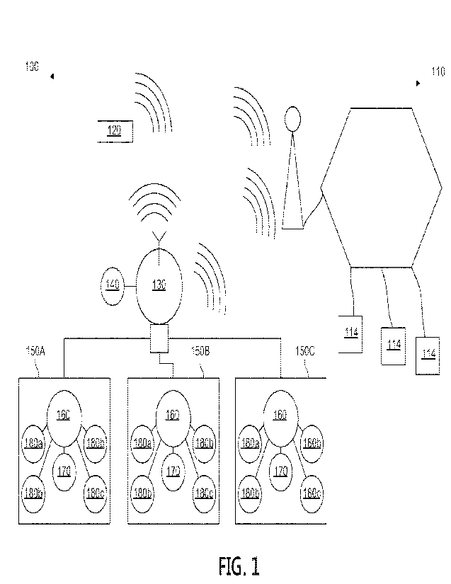
In another embodiment, a system and method for optimized asset health
monitoring that
includes an analytics solution is disclosed.
DESCRIPTION OF RELATED ART
[0003] The use of ultrasonic transducers for ultrasonically
monitoring the condition and
integrity of structural assets, including pipes and pressure vessels, such as
those used in the oil
and gas and power generation industries, is well-known. At present, corrosion
and erosion
monitoring systems and techniques incorporating/using ultrasonic transducers
are known to
1
CA 03201619 2023- 6-7
WO 2022/125059
PCT/US2020/063683
include thickness monitoring at a location and area monitoring (also known as
guided wave
inspection). However, these two systems and techniques are typically separate
from one
another. Moreover, internal corrosion of piping systems is also sometimes
monitored using
radiographic (RT) thickness testing, in addition to ultrasonic (UT) testing,
to measure wall
thicknesses for selected components at prescribed intervals, over the life of
the system.
[0004] Thickness monitoring ultrasonic transducers and systems
utilizing same typically
measure a thickness of a pipe/vessel wall at the spot where the ultrasonic
transducer is provided
¨ in other words, it does not provide any information regarding the thickness
of the pipe/vessel
wall at locations surrounding the exact spot where the ultrasonic transducer
is provided. As
such, if corrosion/erosion is occurring at a location other than where the
ultrasonic transducer
is provided, it is likely that the corrosion/erosion will not be detected,
unless thickness
monitoring is accompanied by ultrasonic transducer mapping. Of course,
ultrasonic transducer
mapping increases the inspection cost. These ultrasonic transducers and
systems are, however,
beneficially permanently installed on pipes/vessels.
[0005] Conversely, area monitoring ultrasonic transducers and
systems utilizing same
typically measure the thickness of a pipe/vessel wall across a larger area of
the pipe/vessel wall,
which area being measured is typically beyond the location where the thickness
monitoring
ultrasonic transducers are provided on the pipe/vessel. Such area monitoring
ultrasonic
transducers and systems utilizing same will typically develop a thickness map
of the pipe/vessel
wall across the area being measured. In theory, such a generated thickness map
is beneficial,
but at present, such guided wave inspection is extremely complex as general
hardware in that
segment generates ten to twenty different guided wave modes, and the high
number of wave
modes and the complex analysis negatively impacts the confidence in the
inspection results.
Further, guided wave inspection is typically not permanently installed on
pipes and vessels.
Additionally, highly localized corrosion cannot be reliably detected with
temporarily installed
guided wave systems as described in API 574 (API 574, Inspection practices for
piping system
components, 4th edition, 2016).
[0006] In addition, existing permanently installed corrosion
monitoring systems fail to use
adequate data to determine the placement of sensors in an industrial facility,
such as an oil
refinery and petrochemical plant, that transport fluids using piping systems.
The piping system
might transport the fluids to one or more tanks and/or chemical processing
unit. Some piping
2
CA 03201619 2023- 6-7
WO 2022/125059
PCT/US2020/063683
systems handle dedicated fluids at prescribed temperatures and/or pressures;
these piping
systems may transfer highly corrosive fluids at elevated temperatures and
pressures.
[0007] Moreover, many industrial facilities face health and safety
concerns. They might
transport fluids that may be flammable and/or toxic. As such, a failure in the
piping system
may cause leakage to the atmosphere and/or exposure to plant personnel.
Moreover, some
facilities operate with no scheduled shutdown for several years. Therefore,
reliability of the
piping system and its components is of importance.
100081 In addition to health and safety concerns, unplanned outages
due to piping system
failures are problematic from a business consequence standpoint. Given the
potential safety,
health, environmental, and business risks associated with piping failures, the
condition of
piping systems is monitored to accurately project their remaining life and
determine safe repair
or replacement dates.
[0009] As a result of the foregoing, certain individuals would
appreciate improvements in
systems and methods for corrosion and erosion monitoring of pipes and vessels.
SUMMARY
[0010] in the following description of various illustrative
embodiments, reference is made
to the accompanying drawings, which form a part hereof, and in which is shown,
by way of
illustration, various embodiments in which aspects of The disclosure may be
practiced Tt is to
be understood that other embodiments may be utilized, and structural and
functional
modifications may be made, without departing from the scope of the present
disclosure. It is
noted that various connections between elements are discussed in the following
description. It
is noted that these connections are general and, unless specified otherwise,
may be direct or
indirect, wired or wireless, and that the specification is not intended to be
limiting in this
respect.
[0011] A system of one or more computers can be configured to
perform particular
operations or actions by virtue of having software, firmware, hardware, or a
combination of
them installed on the system that in operation causes or cause the system to
perform the actions.
One or more computer programs can be configured to perform particular
operations or actions
by virtue of including instructions that, when executed by data processing
apparatus, cause the
apparatus to perform the actions. One general aspect includes a method for
down-selecting
3
CA 03201619 2023- 6-7
WO 2022/125059
PCT/US2020/063683
from among probe assemblies installed on a piping system. The method also
includes setting a
grouping sensitivity hyperparameter, a threshold measurements hyperparameter,
and a
group_size hyperparameter for a model, before training the model. The method
also includes
grouping, by the model executing on a processor, a first set of the probe
assemblies based at
least on historical pipe wall thickness measurements collected from the probe
assemblies
installed on the piping system over a period of time. The method also includes
assigning a
unique groupID to each set of probe assemblies. The method also includes
selecting, by the
model after training the model, an optimization function from among a
plurality of optimization
functions for the model. The method also includes identifying, by the model, a
single probe
assembly corresponding to each groupID for pipe wall thickness monitoring of
the piping
system. The method also includes sending, by a thickness monitoring controller
associated with
the piping system, a pipe wall thickness measurement of the single probe
assembly from each
groupID for inspection. Other embodiments of this aspect include corresponding
computer
systems, apparatus, and computer programs recorded on one or more computer
storage devices,
each configured to perform the actions of the methods.
[0012] Implementations may include one or more of the following
features. The
method may include one or more steps to, during the inspection, disregard all
remaining probe
assemblies in each group1D except the single probe assembly from each group1D.
The grouping
of the first set of the probe assemblies is further based at least on
inspection information
provided to the system and historical pipe wall thickness measurements
collected over a period
of time from the probe assemblies installed on the piping system. The piping
system may
include a tank, and where a first probe assembly of the probe assemblies is
configured to
measure a wall thickness of the tank. The method may also include steps for
storing, in
computer memory communicatively coupled to the processor, historical pipe wall
thickness
measurements collected over an extended period of time from the probe
assemblies installed
on the piping system; and for training, by the processor, the model with at
least the historical
pipe wall thickness measurements stored in the computer memory. The model may
include an
artificial neural network. Implementations of the described techniques may
include hardware,
a method or process, or computer software on a computer-accessible medium.
[0013] One general aspect includes a system for detecting
general corrosion (e.g., a
lack of localized corrosion) to a plurality of components that transport
materials across a
distance. The system may also include a plurality of probe assemblies affixed
to one or more
4
CA 03201619 2023- 6-7
WO 2022/125059
PCT/US2020/063683
of the components, where the probe assemblies may include at least a thickness
monitoring
ultrasonic transducer and an area monitoring ultrasonic transducer configured
to detect
corrosion (e.g., general corrosion and/or localized corrosion) to the
components. The system
may also include a data store configured to store historical wall thickness
measurements
collected over a period of time from measurements performed by the probe
assemblies. The
system may also include a model trained on the historical wall thickness
measurements in the
data store and with hyperparamters may include a grouping_sensitivity
hyperparameter, a
threshold_measurements hyperparameter, and a group_size hyperparameter. The
system may
also include a monitoring apparatus may include a processor and a memory
storing computer-
executable instructions that, when executed by the processor, cause the system
to perform steps
that may also include: grouping, based on the model, a first set of the probe
assemblies;
assigning a unique groupid to each set of probe assemblies; selecting, based
on the model, an
optimization function from among a plurality of optimization functions;
identifying, based on
the model and selected optimization function, a probe assembly corresponding
to each groupid
for wall thickness monitoring of the components: and sending, by a thickness
monitoring
controller associated with the components, a wall thickness measurement of the
probe assembly
from each groupid for inspection. In another embodiment, the system may output
a list of the
unique identifiers corresponding to any groupID in lieu of sending the wall
thickness
measurement for inspection. An inspector may receive the system's output and
react
accordingly, as discussed in various embodiments disclosed herein. Other
embodiments of this
aspect include corresponding computer systems, apparatus, and computer
programs recorded
on one or more computer storage devices, each configured to perform the
actions of the
methods.
100141 Implementations may include one or more of the following
features. The
system, where the probe assembly identified from each groupID, may include
more than one
probe assembly of the plurality of probe assemblies, and where the memory of
the monitoring
apparatus stores computer-executable instructions that, when executed by the
processor, cause
the system to perform steps that may include: during the inspection,
disregarding all remaining
probe assemblies in each groupID except the more than one probe assembly from
each
groupID; and validating that the wall thickness measurements of the more than
one probe
assembly from each groupID is general corrosion and not localized corrosion.
The wall
thickness measurement of the probe assembly from a first groupID may include a
thickness of
a wall of a pipe component at the probe assembly. The wall thickness
measurement of the probe
CA 03201619 2023- 6-7
WO 2022/125059
PCT/US2020/063683
assembly from a first groupID may include a thickness of a wall of a tank
component at the
probe assembly. The method may include validating that the pipe wall thickness
measurement
of the single probe assembly is general corrosion (e.g., a lack of localized
corrosion) by: (i)
generating a probability plot of all pipe wall thickness measurements
associated with the piping
system, (ii) grouping the plotted pipe wall thickness measurements by nominal
thickness, and
(iii) identifying a non-linear relationship in the probability plot of pipe
wall thickness
measurements grouped by nominal thickness to confirm the generalized corrosion
(e.g., lack
of localized corrosion). The pipe wall thickness monitoring may include steps
for, by the probe
assemblies, analyzing the original wall thicknesses, wall thickness loss over
time, calibration
error, and measurement location repeatability error. Implementations of the
described
techniques may include hardware, a method or process, or computer software on
a computer-
accessible medium.
[0015] Implementations may include one or more of the following
features. The
method may further include steps for validating that the pipe wall thickness
measurement of
the single probe assembly is general corrosion (e.g., a lack of localized
corrosion) by:
generating a probability plot of all pipe wall thickness measurements
associated with the piping
system, grouping the plotted pipe wall thickness measurements by nominal
thickness, and
identifying a non-linear relationship in the probability plot of pipe wall
thickness measurements
grouped by nominal thickness to confirm the general corrosion (e.g., the lack
of localized
corrosion). The pipe wall thickness monitoring may include steps, by the probe
assemblies, for
analyzing the original wall thicknesses, wall thickness loss over time,
calibration error, and
measurement location repeatability error. Implementations of the described
techniques may
include hardware, a method or process, or computer software on a computer-
accessible
medium.
BRIEF DESCRIPTION OF THE DRAWINGS
[0016] The present disclosure is illustrated by way of example and
not limited in the
accompanying figures in which like reference numerals indicate similar
elements and in which:
[0017] FIG. 1 is an illustration of the system for
corrosion/erosion monitoring;
[0018] FIG. 2 is an illustration of a thickness monitoring
controller and a piezo assembly of
the system of FIG. 1;
6
CA 03201619 2023- 6-7
WO 2022/125059
PCT/US2020/063683
[0019] FIG. 3 is an illustration of the thickness monitoring
controller of FIG. 2;
[0020] FIG. 4 is an illustration of a switch assembly forming part
of the piezo assembly of
FIG. 2;
[0021] FIG. 5 is an illustration of the piezo assembly of FIG. 2;
[0022] FIG. 6, FIG. 7, and FIG. 8 are illustrations of the method
for corrosion/erosion
monitoring;
[0023] FIG. 9, FIG. 10, FIG. 11, and FIG. 12 are illustrations to
display the signal
modulation;
[0024] FIG. 13A and FIG. 13B (collectively referred to as -FIG.
13") arc drawings of one
illustrative piping with installed MUT sensors in accordance with one or more
aspects of the
features disclosed herein;
[0025] FIG. 14 is an illustrative network architecture of an
industrial facility in accordance
with various aspects of the disclosure;
[0026] FIG. 15 is an illustrative diagram of probe assembly
groupings in one embodiment
of the disclosure;
[0027] FIG. 16A, FIG. 16B, and FIG. 16C (collectively referred to
as "FIG. 16") illustrate
plots on a graph. FIG. 16A is a graph illustrating probability plot of
measurement values for
validating general corrosion in contrast to localized corrosion. FIG. 16B is a
graph charting
level of risk against TMLs in accordance with various aspect disclosed herein.
FIG. 16C
illustrates a shift in the curve depicting the level of risk against TMLs
after down-selection in
accordance with various aspect disclosed herein;
[0028] FIG. 17 is a graph plot of illustrating cumulative thickness
distribution for tubes with
naphthenic acid corrosion;
[0029] FIG. 18A is a corrosion sensor analytics graph illustrating
TML measurements by
date in one embodiment of the disclosure;
[0030] FIG. 18B is another corrosion sensor analytics graph
illustrating TML measurements
by date as in FIG. 8A, but with a higher grouping sensitivity setting;
7
CA 03201619 2023- 6-7
WO 2022/125059
PCT/US2020/063683
[0031] FIG. 18C is yet another corrosion sensor analytics graph
illustrating TML
measurements by date as in FIG. 8A, but with an even higher grouping
sensitivity setting;
[0032] FIG. 19A and FIG. 19B are graphs in accordance with one or
more aspects of the
disclosure;
[0033] FIG. 20A and FIG. 20B are also graphs in accordance with one
or more aspects of
the disclosure;
[0034] FIG. 21 shows an illustrative artificial neural network
configured to operate in
collaboration with systems, methods, and algorithms disclosed herein; and
[0035] FIG. 22 is a flowchart showing illustrative steps of a
method performed in
accordance with some embodiments disclosed herein;
[0036] FIG. 23 is an illustration of a simplified pipe and
instrumentation diagram (PID)
corresponding to an illustrative corrosion/erosion monitoring system, as
illustrated in FIG. 1,
in accordance with some embodiments disclosed herein.
[0037] In the following description of various illustrative
embodimcnts, reference is made
to the accompanying drawings, which form a part hereof, and in which is shown,
by way of
illustration, various embodiments in which aspects of the disclosure may be
practiced. It is to
be understood that other embodiments may be utilized and structural and
functional
modifications may be made, without departing from the scope of the present
disclosure. It is
noted that various connections between elements are discussed in the following
description. It
is noted that these connections arc general and, unless specified otherwise,
may be direct or
indirect, wired or wireless, and that the specification is not intended to be
limiting in this
respect.
8
CA 03201619 2023- 6-7
WO 2022/125059
PCT/US2020/063683
DETAILED DESCRIPTION OF THE PREFERRED EMBODIMENTS
[0038] While the disclosure may be susceptible to embodiment in
different forms, there is
shown in the drawings, and herein will be described in detail, specific
embodiments with the
understanding that the present disclosure is to be considered an
exemplification of the
principles of the disclosure, and is not intended to limit the disclosure to
that as illustrated and
described herein. Therefore, unless otherwise noted, features disclosed herein
may be
combined to form additional combinations that were not otherwise shown for
purposes of
brevity. It will be further appreciated that in some embodiments, one or more
elements
illustrated by way of example in a drawing(s) may be eliminated and/or
substituted with
alternative elements within the scope of the disclosure.
[0039] Aspects of the disclosure relates to the monitoring and
detection of corrosion and/or
erosion of pipes, vessels, and other components in an industrial facility. The
monitoring system
may comprise a software platform for remote monitoring and analytics of
historical
measurements collected by a plurality of sensors affixed to the pipes and
components. The
monitoring system may include analytics tools for monitoring, diagnostics,
and/or prediction
of localized corrosion and/or general corrosion. By using the analytics
systems disclosed
herein, the thickness monitoring locations (TML) may be optimized to, among
other things,
reduce the number of measurement locations without compromising risk¨i.e.,
down-selecting.
Through down-selecting, by strategically reducing the number of probe
assemblies that need
to be sampled during an inspection, the amount of time/cost of an inspection
is reduced while
simultaneously maintaining (or even reducing) the risk profile of the
industrial facility, as
explained in this disclosure.
[0040] A system 100 for monitoring corrosion and erosion of
pipes/vessels is illustrated in
FIG. 1 and FIG. 2. The system 100 includes a data analytics and visualization
platform 110,
an optional gateway 120, a thickness monitoring controller 130, a thickness
monitoring
ultrasonic transducer 140 that is used for standardization purposes, and at
least one probe
assembly 150. Each probe assembly 150 includes a switch assembly 160, at least
one thickness
monitoring ultrasonic transducer 170, and at least one area monitoring
ultrasonic transducer
lgo.
[0041] The data analytics and visualization platform 110 includes a
data analytics portion
112 and a visualization portion 114. 1 The data analytics portion 112 is
typically a cloud-based
9
CA 03201619 2023- 6-7
WO 2022/125059
PCT/US2020/063683
powered software that is configured to receive signals, typically wirelessly,
from one or both
of the gateway 120 or the thickness monitoring controller 130. These signals
are analyzed by
the data analytics portion 112 to translate them into visuals for display on
the visualization
portion 114. The visualization portion 114 may be any suitable device, e.g., a
computer
monitor, a tablet, a phone, etc., that are of a type that will aid an
individual monitoring the
platform 110 in understanding the information regarding corrosion/erosion
identified by the
system 100. The individual may also be able to change the images/information
on the
visualization portion 114 by providing further inputs to the software.
[0042] The gateway 120 may be provided to receive signals,
typically wirelessly, from the
thickness monitoring controller 130, and to send such signals, typically
wirelessly, to the
platform 110. For instance, it may be more economical to use the gateway 120
to establish
cellular connection instead of having each thickness monitoring controller 130
at a facility
having its own data plan. In such a case, the thickness monitoring controllers
130 would use,
e.g., the XBee protocol, to communicate with the gateway 120. In another
example, if there is
no good cellular connection at the location of the thickness monitoring
controller 130, the
gateway 120 could be installed at a higher location to establish cellular
connection and the
thickness monitoring controller 130 would submit data to the gateway 120
using, for example,
the XBee protocol.
[0043] As best illustrated in FIG. 3, the thickness monitoring
controller 130 includes a
modem 131, a microprocessor 132, a pulser 133, an analog-to-digital converter
(ADC) 134, an
adjustable gain amplifier 135, a transmit channel 136, and a receive channel
137. The modem
131 is configured to communicate with one or both of the platform 110 and the
gateway 120.
The modem 131 may use any appropriate communication option, including, but not
limited to
XBee 915 MHz and LTE-M/NB. The modem 131 is configured to communicate with the
microprocessor 132. The microprocessor 132 may be any type of microprocessor
which will
provide the desired functions. One such microprocessor 132 is the LPC4370 that
is
manufactured and sold by NXP Semiconductors. The microprocessor 132 is
configured to
communicate with both the pulser 133 and the ADC 134. The pulser 133 is
preferably a high
voltage pulser capacitor. The ADC 134 is preferably a 16-bit, 2 msps (million
samples per
second), but other ADC types may also be provided as appropriate. The ADC 134
is configured
to communicate with the adjustable gain amplifier 135 (sometimes also commonly
known as a
variable gain amplifier). The adjustable gain amplifier 135 preferably has a
decibel range of
CA 03201619 2023- 6-7
WO 2022/125059
PCT/US2020/063683
26-54 dB and a frequency range of 10 kHZ to 300 kHz, but other ranges may also
be provided
as appropriate. The pulser 133 is configured to communicate with the transmit
channel 136 to
transmit signals to the transmit channel 136. The adjustable gain amplifier
135 is configured
to communicate with the receive channel 137 to receive signals from the
receive channel 137.
The thickness monitoring controller 130 is preferably configured to
accommodate a desired
number of amplitude scans ("A-scans-) (or waveform displays). In the
embodiments
illustrated, the controller 130 is configured to accommodate sixteen A-scans
(one from the
thickness measurement ultrasonic transducer 140 and five each from the three
different probe
assemblies 150). Of course, it is to be understood that as the number of probe
assemblies 150
change and/or the number of ultrasonic transducers 170/180 are included in
each probe
assembly 150 (as will be discussed in further detail below), the controller
130 can be configured
to accommodate more or less than sixteen A-scans as appropriate.
[0044] The thickness monitoring ultrasonic transducer 140 is
configured to receive signals
from the transmit channel 136 of the thickness monitoring controller 130 and
is further
configured to transmit signals to the receive channel 137 of the thickness
monitoring controller
130. As noted, the thickness monitoring ultrasonic transducer 140 is used for
standardization
purposes and, thus, functions to calibrate the measurement system when a group
of ultrasonic
transducers arc utilized (in this instance, the at least one thickness
monitoring ultrasonic
transducer 170, and the at least one area monitoring ultrasonic transducer
180). The
standardization thickness monitoring ultrasonic transducer 140 works to ensure
that the system
100 always performs the same way and functions properly, which is required by
industrial
standards. In the illustrated embodiment, the standardization thickness
monitoring ultrasonic
transducer 140 is configured to perform a single A-scan. in practice, the
thickness monitoring
ultrasonic transducer 140 is typically placed on a standardization block or a
thickness calibrated
metal piece to serve as a standardization transducer.
[0045] As illustrated in FIG. 1, the system 100 includes three
different/distinct probe
assemblies 150A, 150B, 150C (each also referred to as probe assembly 150).
Depending on
the system 100, the number of probe assemblies 150 provided in the system 100
can be less
than three (e.g., one or two) or can be more than three (e.g., four, five,
etc.), as appropriate.
Depending on the number of probe assemblies 150 provided in the system 100,
minor
variations/modifications may need to be made to the system 100 as would be
understood by
one of ordinary skill in the art.
11
CA 03201619 2023- 6-7
WO 2022/125059
PC T/US2020/063683
[0046] As discussed above, each probe assembly 150 includes a
switch assembly 160. As
best illustrated in FIG. 4, the switch assembly 160 includes a power supply
161, a transmit
switch 162, a microcontroller 163, a memory 164, a receive switch 165, an
amplifier 166, and
an optional resistance temperature detector (RTD) interface 167. The power
supply 161 is in
communication with the transmit channel 136 of the thickness monitoring
controller 130. The
transmit switch 162 is in communication with the transmit channel 136 of the
thickness
monitoring controller 130. The transmit switch 162 preferably has five
"switch" channels
162a, 162b, 162c, 162d, 162e, the purpose and function of each will be
discussed herein. The
microcontroller 163 is in communication with the transmit channel 136 of the
thickness
monitoring controller 130, the transmit switch 162, the memory 164, and the
receive switch
165. The microcontroller 163 may be any type of microcontroller which will
provide the
desired functions. One such microcontroller 163 is the PIC18 that is
manufactured and sold by
Microchip Technology. The memory 164 is preferably a non-volatile memory. The
receive
switch 165 preferably has four "switch" channels 165a, 165b, 165c, 165d, the
purpose and
function of each will be discussed hereinbelow. The amplifier 166 is in
communication with
the receive channel 137 of the thickness monitoring controller 130 and the
receive switch 165
The amplifier 166 preferably has an amplification of 26 to 48 dB and a
frequency range of 10
kHz to 300 kHz, but other levels/ranges may also be provided as appropriate.
The amplifier
166 is also preferably a two-stage amplifier, where 26 dB amplification is
provided for a single
stage option and 48 dB amplification is provided for a two-stage option, which
can be selectable
by populating or depopulating components on an amplification board. The
optional RTD
interface 167 is provided if the at least one thickness monitoring ultrasonic
transducer 170
incorporates an RTD 171 (as discussed below). In the illustrated embodiment,
each switch
assembly 160 is instructed by controller 130 to collect five A-scans (one from
the thickness
monitoring ultrasonic transducer 170 and one from each of the four area
monitoring ultrasonic
transducers 180).
[0047] As discussed above, each probe assembly 150 includes at
least one thickness
monitoring ultrasonic transducer 170. As illustrated in FIG. 1, each probe
assembly 150
includes one thickness monitoring ultrasonic transducer 170. Depending on the
system 100
and the probe assembly 150, the number of thickness monitoring ultrasonic
transducers 170
provided in each probe assembly 150 can be more than one (e.g., two, three,
four, etc.), as
appropriate. Depending on the number of thickness monitoring ultrasonic
transducers 170
provided in each probe assembly 150, minor variations/modifications may need
to be made to
12
CA 03201619 2023- 6-7
WO 2022/125059
PCT/US2020/063683
the probe assembly 150 and/or system 100 as would be understood by one of
ordinary skill in
the art. Each thickness monitoring ultrasonic transducer 170 may optionally
have an RTD 171
associated therewith to measure the temperature of the pipe/vessel at or near
where the
thickness measurement is occurring. Each thickness monitoring ultrasonic
transducer 170 is
in communication with the fifth "switch- channel 162e of the transmit switch
162 and, if the
thickness monitoring ultrasonic transducer 170 includes the RTD 171, is also
in communication
with the RTD interface 167.
[0048] The thickness monitoring ultrasonic transducer 170 (as well
as the 140) operates by
generating high frequency ultrasonic waves (e.g., 5 MHz). These ultrasonic
waves are
commonly referred to as longitudinal waves (LW) and, as such, the thickness
monitoring
ultrasonic transducers 170 may also be referred to as LW transducers. In the
illustrated
embodiment, each thickness monitoring ultrasonic transducer 170 is configured
to perform a
single A-scan. Unlike the thickness monitoring ultrasonic transducer 140, the
thickness
monitoring ultrasonic transducer 170 is not placed on a standardization block
or a thickness
calibrated metal piece, but rather is placed on the pipe/vessel to measure the
thickness of the
pipe/vessel at the location where it is installed.
[0049] As discussed above, each probe assembly 150 includes at
least one area monitoring
ultrasonic transducer 180. As illustrated in FIG. 1, FIG. 2, FIG. 3, FIG. 4,
and FIG. 5, each
probe assembly 150 includes four area monitoring ultrasonic transducers 180A,
180B, 180C,
180D (each also referred to as area monitoring ultrasonic transducer 180).
Depending on the
system 100 and the probe assembly 150, the number of area monitoring
ultrasonic transducers
180 provided in each probe assembly 150 can be less than four (e.g., one, two
or three) or more
than four (e.g., five, six, etc.), as appropriate. Depending on the number of
area monitoring
ultrasonic transducers 180 provided in each probe assembly 150, minor
variations/modifications may need to be made to the probe assembly 150 and/or
system 100 as
would be understood by one of ordinary skill in the art. The first area
monitoring ultrasonic
transducer 180A is in communication with the first "switch" channel 162a of
the transmit
switch 162 and the first "switch" channel 165a of the receive switch 165. The
second area
monitoring ultrasonic transducer 180B is in communication with the second
"switch" channel
162b of the transmit switch 162 and the second "switch" channel 165b of the
receive switch
165. The third area monitoring ultrasonic transducer 180C is in communication
with the third
"switch" channel 162c of the transmit switch 162 and the third "switch"
channel 165c of the
13
CA 03201619 2023- 6-7
WO 2022/125059
PCT/US2020/063683
receive switch 165.
The fourth area monitoring ultrasonic transducer 180D is in
communication with the fourth "switch" channel 162d of the transmit switch 162
and the fourth
"switch" channel 165d of the receive switch 165.
[0050]
in an embodiment, the probe assembly 150 may comprise a thickness transducer
170
and a set of area transducers 180 individually wired to switch/preamp assembly
160. In a
different embodiment, thickness and area transducers 170, 180 can be combined
in a single,
larger probe wired via a single multiconductor cable into switch/preamp
assembly 160. In
another embodiment, it also can be a set of larger probes (thickness + 2 area,
area + area etc.)
[0051]
The area monitoring ultrasonic transducers 180 operate by generating low
frequency
ultrasonic waves (e.g., 50 kHz to 500 kHz). These ultrasonic waves are
commonly referred to
as guided waves (GW) and, as such, the area monitoring ultrasonic transducers
180 may also
be referred to as GW transducers. One such type of guided wave, namely shear
horizontal zero
waves (called Silo in plates or T(0,1) in piping), from GW transducers are of
interest due to
their non-dispersive behavior. In the illustrated embodiment, each area
monitoring ultrasonic
transducer 180 is configured to perform a single A-scan.
[0052]
The GW transducers 180 are preferably in the form of piezo patch transducers,
but
may alternatively be in other forms, such as, for instance, face-shear piezo
elements. In a
preferred embodiment, as best illustrated in FIG. 1 and FIG. 5, the GW
transducers 180A,
180B, 180C, 180D are positioned in a rectangular configuration around the LW
transducer 170,
where GW transducer 180A is positioned above and to the left of LW transducer
170, GW
transducer 180B is positioned below and to the left of LW transducer 170, GW
transducer 180C
is positioned below and to the right of LW transducer 170, and GW transducer
180D is
positioned above and to the right of LW transducer 170. When applied to a
pipe/vessel, a
straight line from GW transducer 180A to GW transducer 180B is parallel to a
straight line
from GW transducer 180C to GW transducer 180D, and a straight line from GW
transducer
I 80A to GW transducer 180D is parallel to a straight line from GW transducer
180B to GW
transducer 180C. Further, when applied to a pipe/vessel, a straight line from
GW transducer
180A to GW transducer 180C intersects LW transducer 170, and a straight line
from GW
transducer 180B to GW transducer 180D intersects LW transducer 170, such that
an "X-shape"
configuration is provided.
14
CA 03201619 2023- 6-7
WO 2022/125059
PCT/US2020/063683
[0053] The system 100, when associated with a pipe/vessel, may be
utilized to measure the
corrosion/erosion of the pipe/vessel. In an embodiment, one method 200 of
measuring the
corrosion/erosion of the pipe/vessel is described below and illustrated in
FIG. 6, FIG. 7, and
FIG. 8.
100541 The method 200 includes the step 205 of manually measuring
the actual longitudinal
velocity and the temperature of the pipe/vessel to be inspected.
[0055] The method 200 includes the step 210 of manually measuring
the actual guided wave
velocity and the temperature of the pipe/vessel to be inspected.
[0056] The method 200 includes the step 215 of performing a
thickness standardization
measurement with the standardization thickness monitoring ultrasonic
transducer 140 and the
RTD 171 (it is to be understood that, like the thickness monitoring ultrasonic
transducer 170,
the standardization thickness monitoring ultrasonic transducer 140 could also
optionally
incorporate the RTD 171).
[0057] The method 200 includes the step 220 of performing
measurements using the probe
assembly 150A. Step 220 includes the sub-step 220a of performing a thickness
measurement
with the thickness monitoring ultrasonic transducer 170 and the RTD 171. Step
220 includes
the sub-step 220b of performing an area thickness monitoring with the area
monitoring
ultrasonic transducers 180A, 180B, 180C, 180D at a first frequency. Sub-step
220b includes
the sub-step 220b1 of performing axial scanning whereby area monitoring
ultrasonic transducer
180A is excited and data is recorded with area monitoring ultrasonic
transducer 180B. The
measurement taken in sub-step 220b1 is repeated as often as specified in
configuration setting
and average A-scans. Sub-step 220b includes the sub-step 220b2 of performing
axial scanning
whereby area monitoring ultrasonic transducer 180C is excited and data is
recorded with area
monitoring ultrasonic transducer 180D. The measurement taken in sub-step 220b2
is repeated
as often as specified in configuration setting and average A-scans. Sub-step
220b includes the
sub-step 220b3 of performing circumferential scanning whereby area monitoring
ultrasonic
transducer 180A is excited and data is recorded with area monitoring
ultrasonic transducer
180D. The measurement taken in sub-step 220b3 is repeated as often as
specified in
configuration setting and average A-scans. Sub-step 220b includes the sub-step
220b4 of
performing circumferential scanning whereby area monitoring ultrasonic
transducer 180C is
excited and data is recorded with area monitoring ultrasonic transducer 180C.
The
CA 03201619 2023- 6-7
WO 2022/125059
PCT/US2020/063683
measurement taken in sub-step 220b4 is repeated as often as specified in
configuration setting
and average A-scans. Thus, channels 162a, 162c (which are associated with GW
transducers
180A, 180C) act as guided wave transmit channels while channels 162b, 162d
(which are
associated with GW transducers 180B, 180D) act as guided wave receive
channels. The receive
path further goes via the amplifier 166 to the receive channel 137 of the
thickness monitoring
controller 130.
[0058] Step 220 includes the sub-step 220c of repeating sub-step
220b at a second
frequency, which second frequency is different from the first frequency.
[0059] Step 220 includes the sub-step 220d of repeating sub-step
220b at a third frequency,
which third frequency is different from both the first frequency and the
second frequency.
[0060] The method 200 includes the step 225, which comprises
repeating step 220 to
perform measurements using the probe assembly 150B.
[0061] The method 200 includes the step 230, which comprises
repeating step 220 to
perform measurements using the probe assembly 150C.
[0062] Thus, the method 200 combines ultrasonic thickness
monitoring using longitudinal
waves with ultrasonic area monitoring using guided waves and, in a preferred
embodiment,
just one special non-dispersive shear wave mode (SHo or T(0,1)). The method
200 takes
representative thickness measurements, rather than trying to develop a
thickness map, which
will be complemented by an area monitoring feature to detect localized
corrosion/erosion in-
between representative thickness measurement locations. The system 100
utilizes new
electronics which use a single circuitry to deliver two distinctive, different
excitation signals,
e.g., high frequency ultrasonic waves for thickness monitoring (5 MHz) and low
frequency
ultrasonic waves for area monitoring (50-500 kHz), from two different types of
ultrasonic
transducers, e.g., LW transducer 170 and GW transducers 180. Each excitation
signal needs
to be generated and processed differently. More specifically, pulser 133 of
the controller 130
is a digital switch capable of delivering only predetermined fixed voltage
levels: high voltage,
low voltage and zero voltage. High and low voltage levels are normally
adjustable in a range
of 5V to 90V and -5V to -90V but different voltage levels arc permissible as
well.
Microprocessor 132 signals pulser 133 to output to transmit channel 136 one of
the fixed
voltage levels: ex. high voltage for a specified period of time. Example of a
pulse used to excite
16
CA 03201619 2023- 6-7
WO 2022/125059
PCT/US2020/063683
LW transducer 170: processor 130 instructs pulser 133 to output OV, then high
voltage for a
period of 100ns, then low voltage for a period of 100ns, then OV. Described
sequence would
generate bipolar square wave of 5MHz frequency suitable to excite LW
transducer 170. For
GW transducers 180, different frequencies and signals amplitudes are required.
100631 As best illustrated in FIG. 9, FIG. 10, FIG. 11, and FIG.
12, waveforms needed to
excite GW transducers 180 can have rather complex shapes like, ex: 5 cycle
sinusoid wave
superimposed on Hanning window signal (ex. half cycle cosine) shown as 330 in
FIG. 12 that
would allow for a smoother transition from no-signal to signal condition. To
generate GW
transducer 180 suitable waveforms combination of a pulser 133 digital output
shown as
waveform 300 in FIG. 9, FIG. 10, FIG. 11, and FIG. 12, in-series resistance of
the transmit
channel 136 and impedance of the GW transducer 180 are used. GW transducer 180
impedance
in a frequency range used to generate GW waves (50-500kHz) is usually in
majority composed
of capacitance. This capacitance and mentioned in-series resistance of the
transmit channel 136
form a low pass filter. Pulscr 133 under instructions from the microprocessor
132 generates a
high frequency (usually in range of tens of MHz) digital waveform 300 that
when passed thru
the transmit channel 136 and GW transducer 180 capacitance results in a
different waveform
310 than originally outputted from the pulser 133 (as illustrated in FIG. 10).
Varying high
frequency digital waveforms from the pulser 133 can generate, once passed thru
the transmit
channel 136 in-series resistance and transducer 180 capacitance, a range of
analog waveforms,
ex: sinusoids without Harming windows, shown as 320 in FIG. 11 or sinusoids
with Hanning
windows, shown as 330 in FIG. 12, chirp (frequency changes during duration of
the pulse),
ramp-up, seesaw and other. Of course, other waveforms than those as described
and illustrated
could also be generated.
[0064] In an embodiment, a chirp signal can be used to excite
multiple frequencies at the
same time from a single channel. Proper software filtering can decode the
individual frequency
response from a single A-scan.
[0065] By using the system 100 and method 200, the time of flight
and the amplitude of the
echo reflected at a defect on the pipe/vessel can be evaluated. More
specifically, by sending
excitation signals from GW transducer 180C and receiving by GW transducers
180B, 180D,
the reflection echo will be earlier in time trace in the GW transducer 180B,
180D that is closer
to the damage, e.g., GW transducer 180B if the damage is to the left of both
GW transducers
180B, 180D, or GW transducer 180D if the damage is to the right of both GW
transducers
17
CA 03201619 2023- 6-7
WO 2022/125059
PCT/US2020/063683
180B, 180D, where GW transducers 180B, 180D are positioned as illustrated in
FIG. 1 and
FIG. 5. Defects as pittings or corrosion/erosion patches usually increase in
size over time.
Therefore, the amplitude of the echoes reflected at the defects will increase
over time.
Permanently installed systems therefore allow one to monitor the change of
amplitude next to
the time-of-flight. Monitoring changes in A-Scans after for example baseline
subtraction and
digital filtering reduces the complexity of the analysis and increases
confidence in the
inspection results. Next to baseline subtraction additional digital signal
processing tools or
machine learning algorithms can be used for feature extraction or pattern
recognition which
additionally increase confidence levels and help to detect changes earlier in
time.
[0066] FIG. 23 illustrates a simplified pipe and instrumentation
diagram (PID)
corresponding to an illustrative corrosion/erosion monitoring system, as
illustrated in FIG. I,
in accordance with some embodiments disclosed herein. The simplified PID 2300
includes
numerous probe assemblies depicted as circles numbered nineteen to eighty-
four. For example,
three different/distinct probe assemblies 150A, 150B, 150C arc illustrated. Of
course, the
number of probe assemblies in the PID 2300 can be any number, as appropriate.
In one
example, a human operator/inspector may focus the inspection on a down-
selected list of
TMLs, as explained herein. These down-selected TMLs may represent more
efficient candidate
measuring locations to capture general corrosion behavior of the entire asset,
while still being
able to inspect for localized corrosion. For example, substantial amount of
time/energy and
cost may be saved by down-selecting the number of TMLs so that only those
probe assemblies
with the highest probability of detecting localized corrosion are examined by
the human
operator/inspector. Rather than checking all of probe assemblies nineteen to
eighty-four, or
even randomly checking less than all of probe assemblies nineteen to eighty-
four, the down-
selected TMLs are a more optimal identification of which TMLs to measure. In
some
examples, the inspector may use a handheld or other manual device to measure
wall thickness
at the numbered locations on the simplified PID 2300. In other examples, a rig
or harness of
sorts may be pre-installed at the numbered location on the simplified PID 2300
to allow the
inspector to measure wall thickness at each thickness measuring location. In
yet another
example, the inspector may be an automated machine that takes measurements at
the down-
selected TMLs at particular time intervals. Even in an automated measuring
system, down-
selecting TMLs is advantageous because it reduces the amount of processing
power and
network bandwidth consumed by measurement data generated by a measuring device
at each
numbered location on the simplified PID 2300. For example, some large
industrial facilities
18
CA 03201619 2023- 6-7
WO 2022/125059
PCT/US2020/063683
may have thousands upon thousands of probe assemblies that could result in a
prohibitive
amount of generated data. In addition, once any localized corrosion has been
confirmed and
repaired, a human operator may indicate as much so that any model can be
updated to reflect
the new wall thickness values. In addition, in some examples, if a localized
corrosion is
erroneously identified, then supervised human input into a machine learning or
neural network,
which is executing in a digital analytics platform, may refine its alerts and
model accordingly.
[0067] FIG. 13A illustrates an illustrative piping with sensors
1301 installed on the pipe in
accordance with one or more aspects of the features disclosed herein. The pipe
may have a
flow of liquid in the direction depicted by the arrows. During an inspection,
one approach may
be to inspect and take measurements from each and every sensor 1 to 6 depicted
in FIG. 13A.
in another example, a random selection of sensors may be inspected and
measured. In
accordance with several of the systems and methods disclosed herein, in
another example, the
plurality of thickness monitoring locations (TMLs) shown at each sensor 1 to 6
may be
intelligently considered and a smaller/narrower set of TMLs may be down-
selected for
inspection. Moreover, in accordance with several of the systems and methods
disclosed herein,
the TMLs may be grouped based on one or more criteria in the process of down-
selecting the
TMLs. The down-selecting criteria may, in one simplified example, identify and
exclude those
sensors (e.g., sensors 1 and 3) that historically measured only general
corrosion in its area.
Thus, by down-selecting the system 100 avoids using clustering, but instead
uses grouping to
down-select some sensors as being superfluous to the assessment of the health
of the
mechanical component. Thus, saving time and resources. In contrast, some prior
systems
attempted to reduce risk by adding more TMLs and inspections of those TMLs.
However, the
risk-based inspection (RBT) approach described in various aspects of this
disclosure provides
a superior process and system. An RBI approach may also use a model that takes
into
consideration other criteria such as the type of fluid being transported in
the piping system, the
temperature inside and outside of the pipes/components, elbow/configuration of
the piping
components, and other criteria. For example, the measurements at an elbow may
be weighted
to be more likely to be selected as part of down-selecting in a group because
historically, the
locations near an elbow in piping is a place that will have more turbulence
and friction, thus a
possibility of higher corrosion and acidity.
[0068] Referring to FIG. 13B, probe assemblies 1302 may comprise a
tethered device that
captures accurate spot measurements of thickness of components. In another
embodiment,
19
CA 03201619 2023- 6-7
WO 2022/125059
PCT/US2020/063683
probe assemblies may comprise a tethered device that captures accurate spot
measurements
and area monitoring. For example, the device in FIG. 13B or comparable devices
may be used
to capture area monitoring of the thickness of a pipe component. In yet
another embodiment,
the probe assembly may comprise a wireless device that captures accurate spot
measurements
without necessarily being in direct contact with a piping component that
requires thickness
monitoring. The probe assemblies may comprise one or more of thickness
monitoring
ultrasonic transducers, area monitoring ultrasonic transducers, and/or a
combination thereof
that are configured to validate general corrosion (e.g., confirm no detection
of localized
corrosion) in the piping system.
[0069] FIG. 13B is a drawing of an illustrative piping with
installed sensors. The sensors
1302 may be any of various types of sensors configured to measure a thickness
of the piping
at or near the vicinity of the point of its installation on the pipe. The
sensors 1302 are typically
installed in a permanent location and remains affixed to the pipe for an
extended period of time
(e.g., for the lifespan of that circuit of the piping, for over five years,
for over three years, or
other period of time). Although the sensors 1302 displayed in FIG. 13B are
installed to the
outside of the piping and tethered with wires, in some examples in accordance
with one or more
aspects of the disclosure, the sensors may be untethered and wirelessly
communicate data to
one or more wireless receiver/transceiver devices. In addition, although the
sensors displayed
in FIG. 13B are illustrated in a straight linear pattern along the longitude
of the pipe, the
disclosure contemplates sensors installed in any of several different
patterns. For example, the
density of installed sensors may be based on the direction of gravity and the
type of substance
being transported in the piping. For example, assuming in one example that the
piping in FIG.
13B is transporting a liquid along the length of pipe from the left to the
right when the bottom
of the pipe is the portion of the pipe on which sensor 1302 is installed. In
such an example, the
sensors installed on the piping may be distributed around the circumference of
the piping taking
into consideration that climate conditions (e.g., rain, hail, sun) may expose
portions of the pipe
to greater possibility of deterioration while internal conditions in the
piping (e.g., more liquid
contacts the bottom of the pipe than the top of the pipe) may expose inner
portions of the pipe
to greater possibility of deterioration.
[0070] FIG. 14 is an illustrative network architecture of an
industrial facility with sensors,
communication components, and other components in accordance with various
aspects of the
disclosure. The data analytics platform 112 may be communicatively coupled
over a network,
CA 03201619 2023- 6-7
WO 2022/125059
PCT/US2020/063683
such as a local area network 1408, to one or more networked components. For
example, the
data analytics platform 112 may output to a visualization platform 114 for
generation of one or
more of the illustrative graphs included herein. A monitoring system may
comprise the
software platform 112 to remotely monitor and analyze historical measurements
collected by
a plurality of sensors affixed to the pipes and components. The monitoring
system may include
analytics tools for monitoring, diagnostics, and/or prediction of areas that
are candidates for
localized corrosion (e.g., because the system was unable to confirm general
corrosion to the
area). By using the analytics systems disclosed herein, the TML may be
optimized to, among
other things, reduce the number of measurement locations without compromising
risk¨i.e.,
down-selecting.
[0071] in another example, the data analytics platform 112 may
trigger an alert to be
generated at a remote alert device 1410. The remote alert device 1410 may
result in an
immediate inspection of one or more components, or may result in particular
piping
components being prioritized for a subsequent inspection of the facility.
[0072] As measurements and other data are collected by the systcm
1400, the data may be
stored in a data store 1406 that is communicatively coupled and accessible to
the data analytics
platform 112. In some examples, the data may be stored in computer memory
1404, however,
the amount of computer memory required may be high. Instead, in some examples,
a model
1412, such as a machine learning artificial neural network, may be stored at
the computer
memory 1404 for execution by a processor 1402, while historical data and other
data may be
stored at a data store 1406. In some examples, the data store may be moved
into the platform
112 although it is shown for illustrative purposes as communicating over the
local area network
1408 with the platform 112.
[0073] FIG. 15 is an illustrative diagram of a plurality of sensor
(e.g., probe assembly)
groupings in one embodiment of the disclosure. Each probe assembly may be
assigned a
unique TML identifier (TML ID) as illustrated in FIG. 15. The TML ID may be
any unique
letter, character, or other identifier that uniquely identifies each TML
(i.e., probe assembly).
In FIG. 15, the thick-lined rectangular box around select TML ID numbers shows
probe
assembly groupings. in 1502, on 3-7-2007, the system has grouped probe
assemblies 4, 5, 6,
and 7 into one grouping based on or more rules. In 1504, on 3-7-2008, the
graphical
representation of the data stored in the computer memory 1404 shows that the
system 1400 has
adjusted the grouping to include/exclude one or more TMLs. In 1504, the model
may
21
CA 03201619 2023- 6-7
WO 2022/125059
PCT/US2020/063683
recommend that the probe assembly corresponding to TML ID number four should
no longer
be a part of the groupID corresponding to the thick-lined rectangular box in
1504. As a result,
the one or more probe assembly down-selected for that groupID may also change.
Finally, in
1506, on 3-7-2009, the graphical depiction shows that the system 1400 has
further adjusted the
grouping to now group probe assemblies 5 and 6 into a first groupID and probe
assemblies 7
and 8 to a different/separate second groupID. As a result, the down-selecting
and risk profile,
as illustrated discussed below in FIG. 16, will change for the overall system
100.
[0074] In one example, the grouping of TMLs into a groupID may be
done in one of several
different methods. For example, the initial grouping for each circuit of
components at a facility
may be based on the measurement data level. For every date on which
measurements were
taken by the probe assemblies, a new group may be triggered if a probe
assembly satisfies any
of the following conditions: (i) if the probe assembly is the first TML of the
circuit; (ii) if the
(absolute) difference between the measurement value and the preceding TML's
measurement
value is greater than about 0.5 to about 3.0 standard deviation of all
measurements for that date,
then the value of this parameter may be reduced for more conservative
grouping, or increased
for more aggressive grouping; (iii) if the TML's nominal wall thickness
measurement is
different as compared to the preceding TML's nominal wall thickness
measurement; or if the
TML has only one measurement historically (across all dates). In another
example, the
grouping of TMLs may be done in a multi-step process. In a first step, all
measurements taken
in a group of connected components (e.g., a circuit) on a particular date (or
any other predefined
time period ¨ e.g., within a one-hour window of time, within the same week, or
other) may be
compared to determine how many pairs (or tuples) were measured on the
particular date. In
one example, any TML pairs that have less than a predetermined percentage
(e.g., 70%, 80%,
60%, 75%, or other percent) of the total measurements within that survey year
(or other time
period) are deleted. Next, the minimum measurement value of all the TMLs may
be identified
and all TMLs that were paired in an earlier (e.g., first) step with that TML
are assigned to the
same groupID. Other examples of rules for grouping the TMLs would be apparent
to a person
having skill in the art after review of the entirety disclosed herein.
[0075] Additional other illustrative rules for grouping the TMLs
are contemplated in this
disclosure. For example, in some rules the grouping may be reassigned based on
TML pairing
percentage. For a circuit of components that has at least two measurement
dates, TML pairs
that are grouped together at least a predetermined threshold percentage of
times may be retained
22
CA 03201619 2023- 6-7
WO 2022/125059
PCT/US2020/063683
in the same group, but TMLs that do NOT meet this threshold may be
individually assigned to
separate groups using one or more rules. In yet another example, measurement
dates that do
not have sufficient TMLs may be dropped. For every circuit of components, the
system 1400
may consider, in some examples, only those measurement dates which have at
least a
predetermined threshold percentage of the maximum number of TMLs for any date.
TMLs that
appear in dates that do not meet this threshold may be individually assigned
to separate groups.
[0076] In some examples, the system 1400 may discard (e.g., drop)
seemingly invalid
measurements based on a lack of historical data, and proceed to re-group TMLs
based one or
more of the rules described herein. The thresholds used are hyperparameters
that can be
adjusted based on data set diversity and quality. This adjustment may occur at
the end of the
process upon data confirmation and validation. in one example, threshold
percentage may be
set to 75%, but with some TMLs the prior measurement might not have occurred
in the past,
many years. In some embodiments, a hyper-grid may be generated and used to
adjust the
parameters and/or hyperparameters of the system 1400. In some examples, thc
threshold
setting may be strongly correlated to how many TML measurements a system 1400
has
collected for each TML ID. Thus, the threshold may be adjusted up or down
based on how
much data is made available to the system 1400.
[0077] FIG. 16 and FIG. 17 show graph plots of various data
collected and/or analyzed by
the system 1400. FIG. 16A shows a probability plot graph of measurements
values (normal is
95%) where percentage is on the Y-axis and measurement value is on the X-axis.
The system
1400 defaults to assuming that general corrosion has been detected, except
when the plot shows
that the tail is not running vertical, such as shown near the top of the graph
in FIG. 16A. The
data analytics platform 112 may validate that the pipe wall thickness
measurement of the probe
assembly is general corrosion and not localized corrosion by performing one or
more steps.
For example, in some embodiments, the validating may be performed by
generating a
probability plot of all pipe wall thickness measurements associated with the
piping system,
then grouping the plotted pipe wall thickness measurements by nominal
thickness, and
identifying a non-linear relationship in the probability plot of pipe wall
thickness measurements
grouped by nominal thickness to confirm that the corrosion is likely not
general corrosion.
Meanwhile, where the graph shows a linear relationship, then the TMLs
corresponding to those
data points in the graph are exhibiting general corrosion. This approach is an
advancement
over systems that may have used standard deviation to build normal probability
plots.
23
CA 03201619 2023- 6-7
WO 2022/125059
PCT/US2020/063683
Moreover, the validating step adds further assurance that the system 1400 is
accurately
detecting general corrosion and acting accordingly to down-select the
appropriate probe
assemblies installed on the components in the facility. The system 1400 should
not generate
an alert (e.g., from device 1410) for general corrosion because general
corrosion is pervasive
and is typically not of primary interest during inspections. Rather, general
corrosion is
accounted for in the scheduling and planning for bulk replacement of
components in a facility.
[0078] Referring to FIG. 16B and FIG. 16C, those graphs illustrate
the relationship between
a risk of mis-identifying general corrosion and the quantity of thickness
measurement locations
(TMLs). Although the amount of risk is asymptotic to a threshold minimum
amount of risk
1602 regardless of the number of measurement locations, FIG. 16B shows that
the level of risk
charted against the quantity of probe assemblies (i.e., TMLs) decreases as
more TMLs are
added. Meanwhile, the effects of the system and method disclosed herein are
shown in FIG.
16C, which illustrates a shift in the curve depicting the level of risk
charted against the quantity
of TMLs after down-selection. FIG. 16B and FIG. 16C arc described in more
detail below in
conjunction with the method steps illustrated in the flowchart of FIG. 22.
Meanwhile, FIG. 17
is a graph illustrating cumulative thickness distribution for tubes with
naphthenic acid
corrosion in existing systems known in the art.
[0079] FIG. 18A is a corrosion sensor analytics graph illustrating
TML measurements by
date for a specific circuit ID (or asset ID). The X-axis corresponds to TML
identifiers. For
practical purposes, the probe assemblies installed on a piping system may be
assigned
identifiers in a sequential or otherwise ordered sequence along the circuit
formed by the piping
system. Each TML might have an ID that shows its position upstream or
downstream on the
pipe. Other data cleaning and/or scrubbing of the TMLs based on positional
data may be
performed to harmonize/standardize the measured data for analysis. Each TML
might be
assigned a nominal thickness from when the pipe was first installed. One or
more publicly
available databases (e.g., Meridian database) may provide data, including
nominal thickness
measurements and specifications. Meanwhile, as the legend on the right-hand
side of FIG. 18A
shows, measurements may be taken over a period of time so that historical data
spanning at
least a few years (i.e., an extended period of time) may be stored and
analyzed. In this example,
almost twenty-five years of wall thickness measurement data is stored,
analyzed, and plotted
in FIG. 18A. Graph plot 1802 in FIG. 18A corresponds to measurements taken on
2015-08-
03. Meanwhile, the other plots in the graph correspond to thickness
measurements taken for
24
CA 03201619 2023- 6-7
WO 2022/125059
PCT/US2020/063683
each TML on the corresponding date spanning back almost twenty-five years
(e.g., an extended
period of time).
[0080]
The data analytics platform 112 may set one or more hyperparameter for the
model
1412 corresponding to the graph plotted in FIG. 18A. A hyperparameter is
typically set before
the training/learning process begins on a model; in contrast, the values of
other parameters are
derived through training of the model. In FIG. 18A, a graphical user interface
for adjusting the
grouping_sensitivity hyperparameter is displayed at the top. The visual
platform 114 may
include a graphical tool/slider through which the hyperparameter may be
adjusted. In FIG.
18A, the grouping_sensitivity hyperparameter is shown set to a "standard-
setting. Meanwhile,
in FIG. 18B, which shows another illustration of the model 1412, the
grouping_sensitivity
hyperparameter is shown set to a "medium setting. As a result, the number of
groups is only
sixty-one in FIG. 18B instead of ninety-seven groups in FIG. 18A. In addition,
the graph
plotted 1812 in FIG. 18B is slightly different than the graph 1802 in FIG. 18A
due to the change
in hyperparameter settings and TML selection methods.
Furthermore, with the
grouping_sensitivity hyperparameter set to "high" in FIG. 18C, the graph
plotted 1822 in FIG.
18C is even more different from FIG. 18A and FIG. 18B. The number of groups is
about
seventy-five while the total number of TMLs remains constant at one hundred
fifty-five.
[0081]
The grouping_sensitivity hyperparameter refers to the sensitivity or
aggressiveness
of TML grouping, and may be applied at the initial grouping stage. In some
examples, a TML
may be assigned to a new group when the (absolute) difference between the
measurement value
and the preceding TML's measurement value is greater than 1 standard deviation
(SD) of all
measurements for that date. This threshold can be adjusted for more
conservative or aggressive
grouping. A threshold less than 1 SD will result in the grouping being more
sensitive to
changes in measurements and will lead to a more conservative grouping. On the
other hand, a
threshold greater than 1 SD will cause the grouping being less sensitive to
changes in
measurements and will lead to more aggressive grouping (e.g., higher grouping
ratios). In one
example, five different grouping sensitivities may be implemented, as shown in
FIG. 18C, in
decreasing sensitivity¨from most conservative to most aggressive as follows:
High (0.5 SD),
Standard (1 SD), Medium (1.5 SD), Low (2 SD), and Very Low (3 SD). In another
example,
more or less than the aforementioned five groupings may be used to provide
more granular or
coarse sensitivity. As the grouping_sensitivity hyperparameter is applied at
the initial grouping
stage, as is the case hyperparameters, all subsequent grouping steps may be re-
nm based on the
CA 03201619 2023- 6-7
WO 2022/125059
PCT/US2020/063683
initial grouping results¨i.e., the entire grouping cycle is repeated five
times, once for each of
the five grouping sensitivity levels.
[0082]
Notably, FIG. 18A, FIG. 18B, and FIG. 18C (collectively referred to as "FIG.
18")
list a plurality of TML selection methods that may be applied to the
measurement to optimize
the grouping and plotting of the data points. Although FIG. 18 lists three
optimization
functions¨namely
median TML within group1D,
minimum_average_TML_within_groupID, and minimum_variation_from_mean¨ other
optimization functions may be used in accordance with one or more aspects of
the disclosure.
For example, a TML_position optimization function may be used where if one TML
is to be
selected, the TML at the center of the group is chosen. If two TMLs are to be
selected, the
group is split into two subgroups and the TMLs at the center of each subgroup
are chosen, and
so on. Other examples of TML selection methods are contemplated herein. For
example, the
optimization function may be a minimum_average_TML_vvithin_groupID
optimization
function. In minimum_average_TML_within_group1D method for deciding which
TML(s) to
pick from each group, the method selects the TML(s) having the lowest average
measurement
within each group (across dates). For example, in one illustrative system
using the
minimum_average_TML_within_groupID optimization function, the system may
calculate
average measurement of each TML (across dates), rank TMLs in each group by
(e.g.,
ascending) average measurement, and based on number of TMLs to be picked (n)
from each
group, pick first n TMLs. Likewise, the median_TML_within_groupID optimization
function
is similar to the minimum_average_TML_within_groupID optimization function,
but based on
the median instead of the minimum average.
[0083] In another example the optimization function may be a
minimum_variation_from_mean optimization function. In a
minimum_variation_from_mean
method for deciding which TML(s) to pick from each group, the method selects
the TML(s)
having the lowest average variation from the mean measurement of the group.
For example,
in one illustrative system using the minimum variation from mean optimization
function, the
system may calculate the mean group measurement for each date. Then, for each
TML, for
each date calculate the absolute difference from mean, and for each TML,
calculate the average
variation (e.g., absolute difference from mean). Next, the the
minimum_variation_from_mean
optimization function ranks TMLs in each group by (e.g., ascending) average
variation, and
based on number of TMLs to be picked (n) from each group, pick first n TMLs.
26
CA 03201619 2023- 6-7
WO 2022/125059
PCT/US2020/063683
[0084] After finalizing groupings, the system 1400 determines a TML
candidate selection
method and a desired number of probe assemblies per group. The number of
candidates per
group may be another hyper-parameter. By default, the system 1400 may use the
greater of
1% or one for each TML group. If more than one TML candidate is to be
selected, then the
TML group may be divided into equally big sub-groups while preserving the TML
ordering.
Then, the system 1400 may apply a TML candidate selection method based on the
one or more
scenarios described herein.
[0085] FIG. 19A is a graph 1902 showing the measured TC thickness
in millimeters of a
component over time. Alternatively, the graph may show the values of
temperature calibration
(in Celsius), temperature coefficient (e.g., 1%), corrosion rate ST (in
millimeters per year),
corrosion rate LT (in millimeters per year), remaining life of the component
(in years),
remaining half life (also in years), and the actual thickness (in
millimeters).
[0086] In addition, FIG. 19B is a rectified graph showing FSH (in
percentage) values over
thickness values (in millimeters or other units). The graph also illustrates
the thickness range
of Gate A 1904 and Gate B 1906. Alternatively, the graph may chart the mV
value as a
substitute for FSH. Moreover, in some examples, the graph may be displayed as
HF instead of
rectified.
[0087] FIG. 20A is a graph 2002 of an acid battery facility showing
the measured TC
thickness in millimeters of a component over time. Alternatively, the graph
may show the
values of temperature calibration (in Celsius), temperature coefficient (e.g.,
1%), corrosion rate
ST (in millimeters per year), corrosion rate LT (in millimeters per year),
remaining life of the
component (in years), remaining half life (also in years), and the actual
thickness (in
millimeters). In addition, FIG. 20B is a rectified graph of an acid battery
facility showing FSH
(in percentage) values over thickness values (in millimeters or other units).
The graph also
illustrates the thickness range of Gate A 2004 and Gate B 2006. Alternatively,
the graph may
chart the mV value as a substitute for FSH. Moreover, in some examples, the
graph may be
displayed as HF instead of rectified_
[0088] FIG. 21 illustrates a simplified example of an artificial
neural network 2100 on
which a machine learning algorithm may be executed. FIG. 21 is merely an
example of
nonlinear processing using an artificial neural network; other forms of
nonlinear processing
27
CA 03201619 2023- 6-7
WO 2022/125059
PCT/US2020/063683
may be used to implement a machine learning algorithm in accordance with
features described
herein.
[0089] In FIG. 21, each of input nodes is connected to a first set
of processing nodes. The
external source 2102 which is fed into input nodes may be the metrics from the
results through
the steps of the methods disclosed herein. Each of the first set of processing
nodes is connected
to each of a second set of processing nodes. Each of the second set of
processing nodes is
connected to each of output nodes. Though only two sets of processing nodes
are shown, any
number of processing nodes may be implemented. Similarly, though only four
input nodes,
five processing nodes, and two output nodes per set are shown in FIG. 21, any
number of nodes
may be implemented per set. Data flows in FIG. 21 are depicted from left to
right: data may
be input into an input node, may flow through one or more processing nodes,
and may be output
by an output node. Input into the input nodes may originate from an external
source 2102.
Output 2104 may be sent to a feedback system 2106 and/or to data store. The
feedback system
2106 may send output to the input nodes for successive processing iterations
with the same or
different input data.
[0090] In one illustrative method using feedback system 2106, the
system may use machine
learning to determine an output. The output may include a leak area boundary,
a multi-sensor
detection event, confidence values, and/or classification output. The system
may use an
appropriate machine learning model including xg-boosted decision trees, auto-
encoders,
perceptron, decision trees, support vector machines, regression, and/or a
neural network. The
neural network may be an appropriate type of neural network including a feed
forward network,
radial basis network, recurrent neural network, long/short term memory, gated
recurrent unit,
auto encoder, variational autoencoder, convolutional network, residual
network, Kohonen
network, and/or other type. In one example, the output data in the machine
learning system
may be represented as multi-dimensional arrays, an extension of two-
dimensional tables (such
as matrices) to data with higher dimensionality.
[0091] The neural network may include an input layer, a number of
intermediate layers, and
an output layer. Each layer may have its own weights. The input layer may be
configured to
receive as input one or more feature vectors described herein. The
intermediate layers may be
convolutional layers, pooling layers, dense (fully connected) layers, and/or
other types. The
input layer may pass inputs to the intermediate layers. In one example, each
intermediate layer
may process the output from the previous layer and then pass output to the
next intermediate
28
CA 03201619 2023- 6-7
WO 2022/125059
PCT/US2020/063683
layer. The output layer may be configured to output a classification or a real
value. In one
example, the layers in the neural network may use an activation function such
as a sigmoid
function, a Tanh function, a ReLu function, and/or other functions. Moreover,
the neural
network may include a loss function. A loss function may, in some examples,
measure a
number of missed positives; alternatively, it may also measure a number of
false positives. The
loss function may be used to determine error when comparing an output value
and a target
value. For example, when training the neural network, the output of the output
layer may be
used as a prediction and may be compared with a target value of a training
instance to determine
an error. The error may be used to update weights in each layer of the neural
network.
[0092] In one example, the neural network may include a technique
for updating the weights
in one or more of the layers based on the error. The neural network may use
gradient descent
to update weights. Alternatively, the neural network may use an optimizer to
update weights
in each layer. For example, the optimizer may use various techniques, or
combination of
techniques, to update weights in each layer. When appropriate, the neural
network may include
a mechanism to prevent overfitting¨ regularization (such as Li or L2),
dropout, and/or other
techniques. The neural network may also increase the amount of training data
used to prevent
overfitting.
[0093] In one example, FIG. 21 depicts nodes that may perform
various types of processing,
such as discrete computations, computer programs, and/or mathematical
functions
implemented by a computing device. For example, the input nodes may comprise
logical inputs
of different data sources, such as one or more data servers. The processing
nodes may comprise
parallel processes executing on multiple servers in a data center. And, the
output nodes may
be the logical outputs that ultimately are stored in results data stores, such
as the same or
different data servers as for the input nodes. Notably, the nodes need not be
distinct. For
example, two nodes in any two sets may perform the exact same processing. The
same node
may be repeated for the same or different sets.
[0094] Each of the nodes may be connected to one or more other
nodes. The connections
may connect the output of a node to the input of another node. A connection
may be correlated
with a weighting value. For example, one connection may be weighted as more
important or
significant than another, thereby influencing the degree of further processing
as input traverses
across the artificial neural network. Such connections may be modified such
that the artificial
neural network 2100 may learn and/or be dynamically reconfigured. Though nodes
are
29
CA 03201619 2023- 6-7
WO 2022/125059
PCT/US2020/063683
depicted as having connections only to successive nodes in FIG. 21,
connections may be
formed between any nodes. For example, one processing node may be configured
to send
output to a previous processing node.
[0095] input received in the input nodes may be processed through
processing nodes, such
as the first set of processing nodes and the second set of processing nodes.
The processing may
result in output in output nodes. As depicted by the connections from the
first set of processing
nodes and the second set of processing nodes, processing may comprise multiple
steps or
sequences. For example, the first set of processing nodes may be a rough data
filter, whereas
the second set of processing nodes may be a more detailed data filter.
[0096] The artificial neural network 2100 may be configured to
effectuate decision-making.
As a simplified example for the purposes of explanation, the artificial neural
network 2100 may
be configured to detect faces in photographs. The input nodes may be provided
with a digital
copy of a photograph. The first set of processing nodes may be each configured
to perform
specific steps to remove non-facial content, such as large contiguous sections
of the color red.
The second set of processing nodes may be each configured to look for rough
approximations
of faces, such as facial shapes and skin tones. Multiple subsequent sets may
further refine this
processing, each looking for further more specific tasks, with each node
performing some form
of processing which need not necessarily operate in the furtherance of that
task. The artificial
neural network 2100 may then predict the location on the face. The prediction
may be correct
or incorrect.
[0097] The feedback system 2106 may be configured to determine
whether or not the
artificial neural network 2100 made a correct decision. Feedback may comprise
an indication
of a correct answer and/or an indication of an incorrect answer and/or a
degree of correctness
(e.g., a percentage). For example, in the facial recognition example provided
above, the
feedback system 2106 may be configured to determine if the face was correctly
identified and,
if so, what percentage of the face was correctly identified. The feedback
system may already
know a correct answer, such that the feedback system may train the artificial
neural network
2100 by indicating whether it made a correct decision. The feedback system may
comprise
human input, such as an administrator telling the artificial neural network
2100 whether it made
a correct decision. The feedback system may provide feedback (e.g., an
indication of whether
the previous output was correct or incorrect) to the artificial neural network
2100 via input
nodes or may transmit such information to one or more nodes. The feedback
system may
CA 03201619 2023- 6-7
WO 2022/125059
PCT/US2020/063683
additionally or alternatively be coupled to the storage such that output is
stored. The feedback
system may not have correct answers at all, but instead base feedback on
further processing:
for example, the feedback system may comprise a system programmed to identify
faces, such
that the feedback allows the artificial neural network 2100 to compare its
results to that of a
manually programmed system.
[0098] The artificial neural network 2100 may be dynamically
modified to learn and
provide better input. Based on, for example, previous input and output and
feedback from the
feedback system 2106, the artificial neural network 2100 may modify itself.
For example,
processing in nodes may change and/or connections may be weighted differently.
Following
on the example provided previously, the facial prediction may have been
incorrect because the
photos provided to the algorithm were tinted in a manner which made all faces
look red. As
such, the node which excluded sections of photos containing large contiguous
sections of the
color red could be considered unreliable, and the connections to that node may
be weighted
significantly less. Additionally, or alternatively, the node may be
reconfigured to process
photos differently. The modifications may be predictions and/or guesses by the
artificial neural
network 2100, such that the artificial neural network 2100 may vary its nodes
and connections
to test hypotheses.
[0099] The artificial neural network 2100 need not have a set
number of processing nodes
or number of sets of processing nodes, but may increase or decrease its
complexity. For
example, the artificial neural network 2100 may determine that one or more
processing nodes
are unnecessary or should be repurposed, and either discard or reconfigure the
processing nodes
on that basis. As another example, the artificial neural network 2100 may
determine that
further processing of all or part of the input is required and add additional
processing nodes
and/or sets of processing nodes on that basis.
[0100] The feedback provided by the feedback system 2106 may be
mere reinforcement
(e.g., providing an indication that output is correct or incorrect, awarding
the machine learning
algorithm a number of points, or the like) or may be specific (e.g., providing
the correct output).
For example, the machine learning algorithm may be asked to detect faces in
photographs.
Based on an output, the feedback system may indicate a score (e.g., 75%
accuracy, an
indication that the guess was accurate, or the like) or a specific response
(e.g., specifically
identifying where the face was located). In one example, a human
operator/inspector may
focus the inspection on a down-selected list of TMLs. Once any localized
corrosion has been
31
CA 03201619 2023- 6-7
WO 2022/125059
PCT/US2020/063683
confirmed and repaired, a human operator may indicate as much so that the
model 1412 can be
updated to reflect the new wall thickness values. In addition, in some
examples, a localized
corrosion may be erroneously identified in the system 1400, and supervised
human input into
a machine learning or neural network executing in the digital analytics
platform 112 may refine
its alerts and model accordingly.
101011 The artificial neural network 2100 may be supported or
replaced by other forms of
machine learning. For example, one or more of the nodes of artificial neural
network 2100
may implement a decision tree, associational rule set, logic programming,
regression model,
cluster analysis mechanisms, Bayesian network, propositional formulae,
generative models,
and/or other algorithms or forms of decision-making. The artificial neural
network 2100 may
effectuate deep learning.
[0102] FIG. 22 is a flowchart showing illustrative steps of a
method 2200 performed in
accordance with some embodiments disclosed herein. The method 2200 may be
performed by
a system 1400 when computer-executable instructions, which are stored in a non-
transitory
computer-readable medium, are executed by a processor. The method 2200 may,
among other
things, down-select from among probe assemblies installed on a piping system
in an industrial
facility. As a result, the system and method for optimized asset health
monitoring is improved
because representative measurement locations are identified through down
selection and the
remaining probe assemblies can be disregarded during routine inspections of
the piping system
and other components in an industrial facility.
[0103] Regarding FIG. 22, in step 2202, the system is storing, in a
computer memory 1406
communicatively coupled to the processor 1402, historical pipe wall thickness
measurements
collected over a period of time from the probe assemblies 150A installed on
the piping system
in the industrial facility. In step 2204, the data analytics platform 112 may
set one or more
hyperparameters, such as but not limited to a grouping_sensitivity
hyperparameter, a
threshold_measurements hyperparameter, a group_size hyperparameter, and/or
combination
thereof Once the hyperparameters are set, in step 2206, the system 1400 may
begin training
the model with at least the historical pipe wall thickness measurements stored
in the computer
memory 1406 and hyperparamter values stored in computer memory 1404.
[0104] In step 2208, the model stored in computer memory 1404 may
group a first set of
the probe assemblies from among the numerous probe assemblies installed on the
piping
32
CA 03201619 2023- 6-7
WO 2022/125059
PCT/US2020/063683
system. As explained in this disclosure, such as with respect to FIG. 15,
several methods are
provided by which the grouping may occur in the model. After grouping the
probe assemblies,
the data analytics platform 112 may assign a unique group identifier (groupID)
to each set of
probe assemblies. The unique groupID may be any identifier that the system
1400 can use to
uniquely refer to the group of probe assemblies.
[0105]
In step 2210, the data analytics platform 112 selects, based on at least the
trained
model, an optimization function for the operation of the system 1400. Numerous
illustrative
optimization functions are described in this disclosure, including but not
limited to a
median_TML_within_groupID optimization
function,
minimum_average_TML_within_groupID optimization
function,
mini mum_vari ati on_from_mean optimization function, and/or TM L_po si ti on
optimization
function. The decision to select a specific optimization function causes
subsequent
identification and measurement steps to be effected. For example, in steps
2212A, 2212B,
2212C, and 2212D (collectively "step 2212"), the system 1400 identifies, based
on the model
stored in the computer memory 1404 and selected optimization function, a probe
assembly
corresponding to each groupID for pipe wall thickness monitoring of the piping
system. In
some examples, the system 1400 may identify a single probe assembly for the
entire groupID
to be representative of the area being measured. In other examples, multiple
probe assemblies
may be identified to be representative of the groupID. The number of TMLs
assigned to be
down-selected from a group may be based on one or more rules. This is based on
the value of
the maximum standard deviation of the group, in one example: if any group has
a maximum
standard deviation less than or equal to 0.25, then one TML is chosen from the
group. for an
increase in max SD by 0.25, the number of TMLs selected increases by one
(i.e., if it is between
0.25-0.5, then two probe assemblies may be chosen from the group, and so on).
In addition,
the 0.25 step value can be modified for adjusting the sensitivity of TML
selection. Decreasing
the 0.25 value leads to more TMLs being selected in each group (i.e., a
conservative approach),
and increasing the 0.25 value leads to less TMLs being selected in each group
(i.e., an
aggressive approach).
[0106]
In step 2214, during the inspection, the system 1400 may disregard all
remaining
probe assemblies in each groupID except the probe assembly identified from
each groupID.
The system may measure the wall thickness of each of the identified probe
assemblies for each
groupID, but exclude the other probe assemblies in the groupID. Thus, the
system down-
33
CA 03201619 2023- 6-7
WO 2022/125059
PCT/US2020/063683
selects from among the plurality of probe assemblies installed on a piping
system. At least one
benefit of down-selecting the number of probe assemblies to use during an
inspection is the
time savings that results. For example, a human inspector that might have
previously checked
each probe assembly may now check measurements at a reduced number of probe
assemblies
without substantially increasing the risk of missing dangerous localized
corrosion. In one
example, at step 2214, the system 1400 may output a human-readable report
listing those probe
assemblies a human inspector should manually inspect for wall thickness
measurements. The
output may be ordered in any of various ways¨e.g., based on highest risk of
localized
corrosion, based on geographic convenience from a known start position of the
human
inspector, or other order.
[0107] For example, as illustrated in FIG. 16B and FTG. 16C, when
the amount of risk is
graphed against the quantity of measurement locations taken, the amount of
risk is asymptotic
to a threshold minimum amount of risk 1602 regardless of the number of
measurement
locations increases. Importantly, when the quantity of measurements is
decreased, the delta
change in risk increases at an increasing rate as shown by graph 1604 ¨stated
another way,
reducing the number of probe assemblies that are sampled can increase the risk
to an unsafe
amount. The system 1400 and method 2200 disclosed herein, however, shifts the
graph from
an initial risk graph 1606 to a more favorable risk graph 1608. Therefore,
down-selecting the
number of probe assemblies required to have actively checked during an
inspection, by
identifying those that are the most statistically probable to be general
corrosion/degradation to
the piping wall, results in reduced inspection time/cost while simultaneously
maintaining (or
even reducing) the risk profile.
[0108] Finally, in step 2216 in FIG. 22, the thickness monitoring
controller 130 may receive
and send the pipe wall thickness measurement of the probe assembly from each
groupID for
inspection. The thickness monitoring controller 130 may send the measurement
data (and any
other data) to the data store 1406 for historical recordkeeping and analytics,
as well as to the
data analytics platform 112 for analysis and generation of visualizations. For
example, the wall
thickness measurements may show that a particular segment of pipe in the
piping system is
suffering from degradation other than general corrosion such that it rises to
the level of
dangerous, localized corrosion and must be replaced within a particular period
of time. In
another example, pipe wall thickness measurements may be taken at one or more
of a pipe,
tank, vessel, and/or pipeline at a facility.
34
CA 03201619 2023- 6-7
WO 2022/125059
PCT/US2020/063683
[0109] While particular embodiments are illustrated in and
described with respect to the
drawings, it is envisioned that those skilled in the art may devise various
modifications without
departing from the spirit and scope of the appended claims. It will therefore
be appreciated
that the scope of the disclosure and the appended claims is not limited to the
specific
embodiments illustrated in and discussed with respect to the drawings and that
modifications
and other embodiments are intended to be included within the scope of the
disclosure and
appended drawings. Moreover, although the foregoing descriptions and the
associated
drawings describe example embodiments in the context of certain example
combinations of
elements and/or functions, it should be appreciated that different
combinations of elements
and/or functions may be provided by alternative embodiments without departing
from the
scope of the disclosure and the appended claims. Further, the foregoing
descriptions describe
methods that recite the performance of several steps. Unless stated to the
contrary, one or more
steps within a method may not be required, one or more steps may be performed
in a different
order than as described, and one or more steps may be formed substantially
contemporaneously. Various aspects are capable of other embodiments and of
being practiced
or being carried out in various different ways Tt is to be understood that the
phraseology and
terminology used herein are for the purpose of description and should not be
regarded as
limiting. Rather, the phrases and terms used herein are to be given their
broadest interpretation
and meaning. The use of "including" and "comprising" and variations thereof is
meant to
encompass the items listed thereafter and equivalents thereof as well as
additional items and
equivalents thereof
CA 03201619 2023- 6-7