Note : Les descriptions sont présentées dans la langue officielle dans laquelle elles ont été soumises.
CA 02377602 2001-12-17
WO 01/82216 PCT/US01/13451
MULTI-NEURAL NET IMAGING APPARATUS AND
METHOD
Technical Field
The present invention relates to an imaging apparatus having a plurality of
neural nets, and a method of training the neural nets and a method of
operating such an
imaging apparatus. The apparatus can be used to detect and classify biological
particles
and more particularly, for detecting and classifying biological particles from
human
urine.
BACKGROUND OF THE INVENTION
Biological particle analysis apparatuses are well known in the art. See for
example U.S. Patent No: 4,338,024, assigned to the present assignee, which
describes
a prior art machine that uses a computer having a stored fixed program to
detect and to
classify detected biological particles.
Standard decision theory that is used to sort biological particle images is
well
known, and tends to sort particles by classification in a serial fashion. More
specifically, for a urine sample containing a plurality of particle types, the
particle
images are searched for one or more particle features unique to a single
particle type,
and those images are extracted. This process is repeated for other particles
one particle
type at a time. The problem with this methodology is that each particle type
can
exhibit a range of values for the searched for particle feature(s), and the
range of
values can overlap with those of other particle types. There is also the
problem of
artifacts, which are particle images that have no clinical significance, e.g.
talc or hair,
or cannot be classified due to the sensitivity of the imaging device or other
problems
with the image (e.g. boundary of particle undefined due to partial capture).
Artifact
particle images need to be disregarded from the analysis in such a way as to
not
1
CA 02377602 2010-07-19
79150-25
adversely affect the overall accuracy of the particle analysis. Thus, it can
be difficult
to accurately but reliably classify particles in a sample containing artifacts
.
Most biological particle classification devices further necessitate manual
manipulation to accurately classify the particles in the sample. While
particle features
can be used to segregate particle images by particle type, a trained user is
needed to
verify the result.
Neural net computers are also well known. The advantage of a neural net
computer is its ability to "learn" from its experiences, and thus a neural net
computer,
in theory, can become more intelligent as it is trained.
There is a need for a biological particle classification method and apparatus
for
accurate and automated classification of biological particles in a sample,
such as a
urine sample.
SUMMARY OF THE INVENTION
In some embodiments of the present invention, a multi-neural net image
detecting and classification
apparatus is disclosed. The multi-neural net more efficiently uses the
available
information, which of necessity is finite, in that it more effectively
partitions the
decision space, thereby allowing this information to be used to make fewer
decisions at
each stage while still covering all outcomes with its totality of decisions.
In addition,
the neural net measures certainty at multiple stages of processing in order to
force
images to an abstention class, e.g. artifact. In some sense one can view this
multi.
neural network as forcing the image data to run a gauntlet where at each stage
of the
gauntlet it is quite likely to be placed in an "I don't know" category. This
is much
more powerful than simply.running through a single net because in essence what
is
accomplished is multiple fits of the data to templates which are-much better
defined
than a single template could be because of the more effective use of the
information.
Some embodiments of the present invention also relate to a large set
of particle features and a training method, which involves not simply a single
pass through the training set, but
2
CA 02377602 2011-08-16
'79150-25
selecting from a number of nets and then reducing the feature vector size.
Finally, the
present invention provides for preprocessing and post processing that enables
heuristic
information to be included as part of the decision making process. Post
processing
enables contextual information either available from other sources or gleaned
from the
actual decision making process to be used to further enhance the decisions.
One aspect of the present invention is a method of classifying an element
in an image into
one of a plurality of classification classes, wherein the element has a
plurality of
features. The method includes the steps of extracting the plurality of
features from the
image, determining a classification class of the element, and modifying
the determined classification class of the element based upon a plurality of
previously
determined classification class determinations. The determination of the
element
classification class includes at least one of:
selecting and processing a first subgroup of the extracted features to
determine a physical characteristic of the element, and selecting and
processing
a second subgroup of the extracted features using the physical
characteristic determined to determine a classification class of the element;
and
selecting and processing a third subgroup of the extracted features to
determine a group of classification classes of the element, and selecting and
processing a fourth subgroup of the extracted features using the
determined classification class group to determine a classification class of
the
element.
In other aspect of the present invention, an imaging apparatus for classifying
an
element in an image into one of a plurality of classification classes, wherein
the
element has a plurality of features, includes means for extracting the
plurality of
features from the image, means for determining a classification class of
the element, and means for modifying the determined classification class of
the
element based upon a plurality of previously determined classification class
determinations. The determining means includes at least one of.
3
CA 02377602 2011-08-16
79150-25
means for selecting and processing a first subgroup of the extracted
features to determine a physical characteristic of the element, and means for
selecting and processing a second subgroup of the extracted features
using the physical characteristic determined to determine a classification
class of the element, and
means for selecting and processing a third subgroup of the extracted
features to determine a group of classification classes of the element, and
means for selecting and processing a fourth subgroup of the extracted features
using the determined classification class group to determine a
classification class of the element.
In yet another aspect of the present invention, a method of classifying an
element in an image into one of a plurality of classifications, wherein the
element has a
plurality of features, includes the steps of extracting the plurality of
features from the
image, determining a classification of the element based upon the plurality of
features
extracted by a first determination criteria wherein the first determination
criteria
includes the classification of the element as an unknown classification,
determining a
classification of the element by a second determination criteria, different
from the first
determination criteria, in the event the element is classified as an unknown
classification by the first determination criteria, and determining the
classification of
the element by a third determination criteria, different from the first and
second
determination criteria, in the event the element is classified as one of a
plurality of
classifications by the first determination criteria.
In yet one more aspect of the present invention, an imaging apparatus for
classifying an element in an image into one of a plurality of classification
classes,
wherein the element has a plurality of features, includes: an extractor for
extracting
the plurality of features from the image of the element; a first processor
that
determines a classification class of the element, and a second processor that
modifies
the determined classification class of the element based upon a plurality of
previously
4
CA 02377602 2010-07-19
79150-25
determined classification class determinations. The first processor determines
the
classification class of the element by at least one of:
selecting and processing a first subgroup of the extracted features to
determine a physical characteristic of the element, and selecting and
processing a
second subgroup of the extracted features in response to the physical
characteristic determined to determine a classification class of the element;
and
selecting and processing a third subgroup of the extracted features
to determine a group of classification classes of the element, and selecting
and
processing a fourth subgroup of the extracted features in response to the
determined classification class group to determine a classification class of
the
element.
Other objects and features of embodiments of the present invention
will become apparent by a review of the specification, claims and appended
figures.
BRIEF DESCRIPTION OF DRAWINGS
Figure 1 is a flow diagram showing the method of an embodiment of
the present invention.
Figure 2 is a schematic diagram of the apparatus of an embodiment
of the present invention.
Figures 3A and 3B are flow diagrams illustrating the boundary
enhancement of an embodiment of the present invention.
Figure 4 is a diagram illustrating the symmetry feature extraction of
an embodiment of the present invention.
Figures 5A to 5D are drawings illustrating the skeletonization of
various shapes.
Figure 6A is a flow diagram showing the LPF scan process of an
embodiment of the present invention.
Figure 6B is a flow diagram of the neural net classification used with
the LPF scan process of an embodiment of the present invention.
5
CA 02377602 2010-07-19
79150-25
Figure 7A is a flow diagram showing the HPF scan process of an
embodiment of the present invention.
Figure 7B is a flow diagram of the neural net classification used with
the HPF scan process of an embodiment of the present invention.
Figure 8 is a schematic diagram of the neural net used with an
embodiment of the present invention.
Figures 9A to 9C are tables showing the particle features used with
the various neural nets in the LPF and HPF scan processes of some
embodiments of the present invention.
DETAILED DESCRIPTION
Some embodiments of the present invention comprise a method and
apparatus for making decisions about the classification of individual particle
images in an ensemble of images of biological particles for the purpose of
identifying each individual image, and determining the number of images in
each
given class of particles.
Basic Method and Apparatus
The method is generally shown schematically in Figure 1, and
comprises 5 basic steps:
1) collect individual images,
2) extract particle features from each individual image,
3) apply certain pre-processing rules to determine classifications of
individual images or how the classification process will be performed,
4) classify the individual images using a multiple neural net decision
making structure, and
5) analyze the ensemble of decisions or a subset of the ensemble of
decisions to determine the overall classification of the ensemble or changes
to
classifications of certain subsets or individual images.
6
CA 02377602 2010-07-19
79150-25
The method of the present invention further includes steps that train the
individual neural nets used to make decisions, as well as steps that select
the nets used
in the final decision-making from among multiple nets produced by the training
procedure.
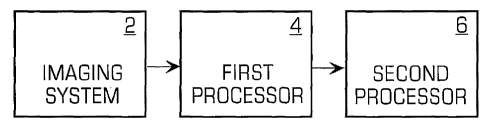
There are three major hardware elements that are used to implement the present
invention: an imaging system 2, a first processor 4 and a second processor 6.
These
hardware elements are schematically illustrated in Fig. 2.
Imaging system 2 is used to produce images of fields of view of a sample
containing the particles of interest. Imaging system 2 is preferably a well
known flow
microscope as described in U.S. Patents 4,338,024, 4,393,466, 4,538,299 and
4,612,614. The flow
microscope produces images of successive fields containing particles as they
flow
through a flow cell.
First processor 4 analyzes the images of successive fields, and isolates the
particles in individual patches. A patch extraction apparatus (such as that
described in
U.S. Patents 4,538,299 and 5,625,709)
is used to analyze the images produced by the imaging system and to define
local areas (patches) containing particles of interest. The boundary of each
particle is
identified and defined, and used to extract the picture data for each particle
from the
larger field, thereby producing digital patch images that each contain the
image of an
individual particle of interest (resulting in a significant compression of the
data
subsequently required for processing). Imaging system 2 and first processor 4
combine to perform the first step (collection of individual images) shown in
Fig. 1.
Second processor 6 analyzes each particle image to determine the
classification
of the particle image. Second processor 6 performs the last four steps shown
in Fig. 1,
as described below.
7
CA 02377602 2010-07-19
79150-25
Boundary Enhancement - Mask Images
To enhance the particle feature extraction, the particle boundary is further
refined, and black and white mask images of the particles are created. This
process
effectively changes all the digital image pixels outside the boundary of the
particle
(background pixels) to black pixels, and the pixels inside the particle
boundary to
white pixels. The resulting white images of the particles against a black
background
conveys the particles' shape and size very clearly, and are easy to operate on
for
particle features based on shape and size only (given that the pixels are
either white or
black).
Figs. 3A-3B illustrate the basic steps for transforming the particle image
into a
mask image. First, a Shen-Castan edge detector (as described in Parker, James
R.,
Algorithms for Image Processing and Computer Vision, ISBN 0-471-14056-2, John
Wiley & Sons, 1997, pp 29-32) is used to define
the edges of particles of interest, as illustrated in Fig. 3A. A particle
image 10
typically contains images of particles of interest 12 and other particles 14.
The particle
image 10 is smoothed, and a band limited Laplacian image is created, followed
by a
gradient image. A threshold routine is used to detect the edges, whereby the
locations
where the intensity crosses a predetermined threshold are defined as edges.
The
detected edges are connected together to result in an edges image 16, which
contains
lines that correspond to detected boundaries that outline the various
particles.
A mask image is created from the edge image 16 in the manner illustrated in
Fig. 3B. The edge image 16 is inverted so the boundary lines are white and the
background is black. Then, the image is cleaned of all small specks and
particles too
small to be of interest. Small gaps in the boundary lines are filled to
connect some of
the boundary lines together. The boundary lines are dilated to increase their
width.
This dilation is on the outer edges of the boundary lines, since the inner
edges define
the actual size of the particles. Disconnected pixels are bridged to create
complete
lines that enclose the particles. The inside of the boundaries are filled in
to create
8
CA 02377602 2001-12-17
WO 01/82216 PCT/US01/13451
blobs that represent the particles. The blobs are eroded to remove the pixels
that had
formed the boundary lines, so that the blobs have the correct size. Finally,
the largest
blob is detected, and all the remaining blobs are discarded. The resulting
image is a
mask image of the particle, where the white blob against the black background
accurately corresponds to the size and shape of the particle of interest.
Particle Feature Extraction
Once the image of a particle of interest has been localized within a patch
image, and its boundary further refined by creating a white mask image of the
particle,
the patch and mask images are further processed in order to extract particle
features
(feature data) from the particle image. Generally, the particle features
numerically
describe the size, shape, texture and color of the particles in numerous
different ways
that aid in the accurate classification of particle type. The particle
features can be
grouped in families that are related to one of these numerical descriptions,
and can be
extracted from the patch image, the mask image, or both.
The first family of particle features all relate to the shape of the particle,
which
aid in differentiating red and white blood cells which tend to be round,
crystals which
tend to be square or rectangular, and casts with tend to be elongated. The
first family
of particle features are:
1. Particle Area: the number of pixels contained within the particle
boundary. Preferably, this particle feature is derived from the mask
image of the particle.
2. Perimeter Length: the length of the particle boundary in pixels.
Preferably, this is derived from the particle mask image by creating a 4-
neighborhood perimeter image of the mask, and counting the number of
non-zero pixels.
9
CA 02377602 2001-12-17
WO 01/82216 PCT/US01/13451
3. Shape Factor: an indication of the roundness of the particle. This is
calculated as the square of the Perimeter Length, divided by the Particle
Area.
4. Area to Perimeter Ratio: another indication of the roundness of the
particle. This is calculated as the Particle Area divided by the Perimeter
.Length.
The second family of particle features relates to the symmetry of the
particle,
and in particular the determination of the number of lines of symmetry for any
given
shaped particle. This family of particle features are quite useful in
distinguishing casts
(typically having a line of symmetry along its long axis) and squamous
epithelial cells
(SQEPs, which generally have no line of symmetry). This family of particle
features
utilizes information derived from line segments applied at different angular
orientations to the particle. As illustrated in Fig. 4, a line segment 20 is
drawn through
the centroid 22 of the mask image 19. For each point along the line segment
20, line
segments 24a and 24b perpendicular thereto are drawn to extend away from the
line
segment 20 until they intersect the particle boundary, and the difference in
length of
the opposing perpendicular line segments 24a and 24b are calculated and
stored. This
calculation is repeated for each point along the line segment 20, where all
the
difference values are then summed and stored as a Symmetry Value for line
segment
20. For a perfect circle, the Symmetry Value is zero for any line segment 20.
The
calculation of the Symmetry Value is then repeated for each angular rotation
of line
segment 20, resulting in a plurality of Symmetry Values, each one
corresponding to a
particular angular orientation of line segment 20. The Symmetry Values are
then
normalized by the Particle Area value, and sorted into an ordered list of
Symmetry
Values from low to high.
The second family of particle features are:
CA 02377602 2010-07-19
79150-25
5. Minimum Symmetry: the lowest Symmetry Value in the ordered list,
which represents the maximum symmetry exhibited by the particle at
some value of rotation.
6. 20% Symmetry: the Symmetry Value that constitutes the 20th percentile
of the ordered list of Symmetry Values.
7. 50% Symmetry: the Symmetry Value that constitutes the 50th percentile
of the ordered list of Symmetry Values.
8. 80% Symmetry: the Symmetry Value that constitutes the 80th percentile
of the ordered list of Symmetry Values.
9. Maximum Symmetry: the highest Symmetry Value in the ordered list,
which represents the minimum symmetry exhibited by the particle at
some value of rotation.
10. Average Symmetry: the average value of the Symmetry Values.
11. Standard Deviation Symmetry: the standard deviation of the Symmetry
Values.
The third family of particle features relate to skeletonization of the
particle
image, which produces one or more line segments that characterize both the
size and
the shape of the particle. These particle features are ideal in identifying
analytes
having multiple components in a cluster, such as budding yeast, hyphae yeast,
and
white blood cell clumps. These analytes will have skeletons with multiple
branches,
which are easy to differentiate from analytes having single branch skeletons.
Creation
of skeleton images is well known in the art of image processing, and is
disclosed in
Parker, James R, Algorithms for Image Processing and Computer Vision, ISBN 0-
471-14056-2, John Wiley & Sons, 1997, pp 176-210).
Skeletonization essentially involves collapsing each portion of the
particle boundary inwardly in a direction perpendicular to itself. For
example, a
perfect circle collapses to a single point; a crescent moon collapses to a
curved line, a
figure-8 collapses to 2 straight line segments, and a cell with an indentation
collapses
11
CA 02377602 2001-12-17
WO 01/82216 PCT/US01/13451
to a curved line, as illustrated in Figs. 5A - 5D respectively. The preferred
embodiment utilizes two skeletonization algorithms: ZSH and BZS. ZSH is the
Zhang-Suen thinning algorithm using Holt's variation plus staircase removal.
BZS is
the Zhang-Suen thinning algorithm using Holt's variation. Figure 5.11 in
Parker (p.
182) shows the difference between results when these algorithms are applied,
along
with C-code for each algorithm.
The third family of particle features are:
12. ZSH Skeleton Size: the size of the skeleton, preferably determined by
counting the number of pixels forming the skeleton. The Skeleton Size
for a perfect circle is 1, and for a crescent moon would be the length of
the curved line.
13. ZSH Normalized Skeleton Size: Skeleton Size normalized by the size of
the particle, determined by dividing Skeleton Size by Particle Area.
14. BZS Skeleton Size: the size of the skeleton, preferably determined by
counting the number of pixels forming the skeleton. The Skeleton Size
for a perfect circle is 1, and for a crescent moon would be the length of
the curved line.
15. BZS Normalized Skeleton Size: Skeleton Size normalized by the size of
the particle, determined by dividing Skeleton Size by Particle Area.
The fourth family of particle features relate to measuring the shape of the
particle using radial lengths of radii that fit in the particle, and the
quantile rankings of
these values. Specifically, a centroid is defined inside the particle,
preferably using the
mask image, and a plurality of radii emanating from the centroid at different
angles
extend out to the particle boundary. The lengths of the radii are collected
into a list of
Radii Values, and the list is sorted from low to high values. A certain %
quantile of an
ordered list of values represents the value having a position in the list that
corresponds
12
CA 02377602 2001-12-17
WO 01/82216 PCT/US01/13451
to the certain percentage from the bottom of the list. For example, a 30%
quantile of a
list is the value that is positioned 30% up from bottom of the list, with 70%
of the
values being above it in the list. So, in an order list of 10 values, the 30%
quantile
value is the seventh value from the top of the list, and the 50% quantile is
the median
value of the list.
The fourth family of particle features are:
16. 25% Radii Value: the value corresponding to the 25% quantile of the list
of Radii Values.
17. 50% Radii Value: the value corresponding to the 50% quantile of the list
of Radii Values.
18. 75% Radii Value: the value corresponding to the 75% quantile of the list
of Radii Values.
19. Smallest Mean Ratio: the ratio of the smallest Radii Value to the mean
Radii Value.
20. Largest Mean Ratio: the ratio of the largest Radii Value to the mean
Radii Value.
21. Average Radii Value: the average of the Radii Values.
22. Standard Deviation Radii Value: the standard deviation of the Radii
Values.
The fifth family of particle features measures the intensity of the particle
image. Light absorption properties of different analytes differ significantly.
For
example, crystals are generally refractive and may actually "concentrate"
light so that
their interior may be brighter than the background. Stained white blood cells,
however, will typically be substantially darker than the background. The
average
intensity reveals the overall light absorbing quality of the particle, while
the standard
deviation of intensity measures the uniformity of the particle's absorbing
quality. In
order to measure intensity, the particle is preferably isolated by using the
mask image
13
CA 02377602 2001-12-17
WO 01/82216 PCT/US01/13451
in order to mask the patch image of the particle. Thus, the only pixels left
(inside the
mask) are those pixels contained inside the particle boundary. This family of
particle
features includes:
23. Average Pixel Value: the average pixel value for all the pixels inside the
particle boundary.
24. Standard Deviation of Pixel Values: the standard deviation of pixel
values for pixels inside the particle boundary.
The sixth family of particle features use the Fourier Transform of the
particle to
measure the radial distribution of the particle. The Fourier Transform depends
on the
size, shape and texture (i.e. fine grain structure) of the particle. In
addition to adding
texture, the Fourier Transform magnitude is independent of the position of the
particle,
and particle rotation is directly reflected as a rotation of the transform.
Finding
clusters of energy at one rotation is an indication of linear aspects of the
particle (i.e.
the particle has linear portions). This finding helps discriminate between
particles such
as crystals versus red blood cells. The Fourier Transform of the patch image
of the
particle is preferably calculated using a well known Fast Fourier Transform
(FFT)
algorithm with a window of 128x128 pixels. The following particle features are
then
calculated:
25. FFT Average Intensity of Rotated 128 Pixel Line: a queue listing of
average pixel values along a 128 pixel line as a function of rotation angle.
This is calculated by placing a radial line of length 128 pixels over the
transform, and rotating the radial line through an arc of 180 degrees by
increments of N degrees. For each increment of N degrees, the average
of the pixel values along the radial line is calculated. The average pixel
values for the N degree increments are stored in a queue as Average
Intensity along with the corresponding angular increment.
14
CA 02377602 2001-12-17
WO 01/82216 PCT/US01/13451
26. FFT Maximum/Minimum. 128 Pixel Angular Difference: the difference
between the angular values that correspond to the highest and lowest
Average Intensity values stored in the queue.
27. FFT 128 Pixel Average Intensity Standard Deviation: the standard
deviation of the Average Intensity values stored in the queue.
28. FFT Average Intensity of Rotated 64 Pixel Line: same as the FFT
Average Intensity of Rotated 128 Pixel Line, but instead using a 64 pixel
length radial line.
29. FFT Maximum/Minimum 64 Pixel Angular Difference: same as the FFT
Maximum/Minimum 128 Pixel Angular Difference, but instead using a
64 pixel length radial line.
30. FFT 64 Pixel Average Intensity Standard Deviation: same as the FFT 128
Pixel Average Intensity Standard Deviation, but instead using a 64 pixel
length radial line.
31. FFT Average Intensity of Rotated 32 Pixel Line: same as the FFT
Average Intensity of Rotated 128 Pixel Line, but instead using a 32 pixel
length radial line.
32. FFT Maximum/Minimum 32 Pixel Angular Difference: same as the FFT
Maximum/Minimum 128 Pixel Angular Difference, but instead using a
32 pixel length radial line.
CA 02377602 2001-12-17
WO 01/82216 PCT/US01/13451
33. FFT 32 Pixel Average Intensity Standard Deviation: same as the FFT 128
Pixel Average Intensity Standard Deviation, but instead using a 32 pixel
length radial line.
Additional FFT particle features all related to standard deviation values
based
upon a rotated radial line of varying lengths are as follows:
34. FFT 128 Pixel Average Intensity Standard Deviation Sort: a sorted queue
listing of the standard deviation of average pixel values along a 128 pixel
line for different rotations. This is calculated by placing a radial line of
length 128 pixels over the transform, and rotating the radial line through
an arc of 180 degrees by increments of N degrees. For each increment of
N degrees, the standard deviation value of the pixels on the line is
calculated. The standard deviation values for all the N degree increments
are sorted from low to high, and stored in a queue.
35. FFT 128 Pixel Minimum Radial Standard Deviation: the minimum radial
standard deviation value retrieved from the sorted queue listing of
standard deviation values.
36. FFT 128 Pixel Maximum Radial Standard Deviation: the maximum radial
standard deviation value retrieved from the sorted queue listing of
standard deviation values.
37. FFT 128 Pixel 25% Quantile Radial Standard Deviation: the radial
standard deviation value from the queue corresponding to the 25%
quantile of the values stored in the queue.
16
CA 02377602 2001-12-17
WO 01/82216 PCT/US01/13451
38. FFT 128 Pixel 50% Quantile Radial Standard Deviation: the radial
standard deviation value from the queue corresponding to the 50%
quantile of the values stored in the queue.
39. FFT 128 Pixel 75% Quantile Radial Standard Deviation: the radial
standard deviation value from the queue corresponding to the 75%
quantile of the values stored in the queue.
40. FFT 128 Pixel Minimum to Average Radial Standard Deviation Ratio: the
ratio of the minimum to average radial standard deviation values stored in
the queue.
41. FFT 128 Pixel Maximum to Average Radial Standard Deviation Ratio:
the ratio of the maximum to average radial standard deviation values
stored in the queue.
42. FFT 128 Pixel Average Radial Standard Deviation: the average radial
standard deviation value of the values stored in the queue.
43. FFT 128 Pixel Standard Deviation of the Radial Standard Deviation: the
standard deviation of all of the radial standard deviation values stored in
the queue.
44. FFT 64 Pixel Average Intensity Standard Deviation Sort: the same as the
FFT 128 Pixel Average Intensity Standard Deviation Sort, but instead
using a 64 pixel length radial line.
17
CA 02377602 2001-12-17
WO 01/82216 PCT/US01/13451
45. FFT 64 Pixel Minimum Radial Standard Deviation: the same as the FFT
128 Pixel Minimum Radial Standard Deviation, but instead using a 64
pixel'length radial line.
46. FFT 64 Pixel Maximum Radial Standard Deviation: the same as the FFT
128 Pixel Maximum Radial Standard Deviation, but instead using a 64
pixel length radial line.
47. FFT 64 Pixel 25% Quantile Radial Standard Deviation: the same as the
FFT 128 Pixel 25% Quantile Radial Standard Deviation, but instead using
a 64 pixel length radial line.
48. FFT 64 Pixel 50% Quantile Radial Standard Deviation: the same as the
FFT 128 Pixel 50% Quantile Radial Standard Deviation, but instead using
a 64 pixel length radial line.
49. FFT 64 Pixel 75% Quantile Radial Standard Deviation: the same as the
FFT 128 Pixel 75% Quantile Radial Standard Deviation, but instead using
a 64 pixel length radial line.
50. FFT 64 Pixel Minimum to Average Radial Standard Deviation Ratio: the
same as the FFT 128 Pixel Minimum to Average Radial Standard
Deviation Ratio, but instead using a 64 pixel length radial line.
51. FFT 64 Pixel Maximum to Average Radial Standard Deviation Ratio: the
same as the FFT 128 Pixel Maximum to Average Radial Standard
Deviation Ratio, but instead using a 64 pixel length radial line.
18
CA 02377602 2001-12-17
WO 01/82216 PCT/US01/13451
52. FFT 64 Pixel Average Radial Standard Deviation: the same as the FFT
128 Pixel Average Radial Standard Deviation, but instead using a 64
pixel length radial line.
53. FFT 64 Pixel Standard Deviation of the Radial Standard Deviation: the
same as the FFT 128 Pixel Standard Deviation of the Radial Standard
Deviation, but instead using a 64 pixel length radial line.
54. FFT 32 Pixel Average Intensity Standard Deviation Sort: the same as the
FFT 128 Pixel Average Intensity Standard Deviation Sort, but instead
using a 32 pixel length radial line.
55. FFT 32 Pixel Minimum Radial Standard Deviation: the same as the FFT
128 Pixel Minimum Radial Standard Deviation, but instead using a 32
pixel length radial line.
56. FFT 32 Pixel Maximum Radial Standard Deviation: the same as the FFT
128 Pixel Maximum Radial Standard Deviation, but instead using a 32
pixel length radial line.
57. FFT 32 Pixel 25% Quantile Radial Standard Deviation: the same as the
FFT 128 Pixel 25% Quantile Radial Standard Deviation, but instead using
a 32 pixel length radial line.
58. FFT 32 Pixel 50% Quantile Radial Standard Deviation: the same as the
FFT 128 Pixel 50% Quantile Radial Standard Deviation, but instead using
a 32 pixel length radial line.
19
CA 02377602 2001-12-17
WO 01/82216 PCT/US01/13451
59. FFT 32 Pixel 75% Quantile Radial Standard Deviation: the same as the
FFT 128 Pixel 75% Quantile Radial Standard Deviation, but instead using
a 32 pixel length radial line.
60. FFT 32 Pixel Minimum to Average Radial Standard Deviation Ratio: the
same as the FFT 128 Pixel Minimum to Average Radial Standard
Deviation Ratio, but instead using a 32 pixel length radial line.
61. FFT 32 Pixel Maximum to Average Radial Standard Deviation Ratio: the
same as the FFT 128 Pixel Maximum to Average Radial Standard
Deviation Ratio, but instead using a 32 pixel length radial line.
62. FFT 32 Pixel Average Radial Standard Deviation: the same as the FFT
128 Pixel Average Radial Standard Deviation, but instead using a 32
pixel length radial line.
63. FFT 32 Pixel Standard Deviation of the Radial Standard Deviation: the
same as the FFT 128 Pixel Standard Deviation of the Radial Standard
Deviation, but instead using a 32 pixel length radial line.
Even more FFT particle features are used, all related to average values based
upon a rotated radial line of varying lengths:
64. FFT 128 Pixel Average Intensity Sort: a sorted queue listing of the
average pixel values along a 128 pixel line for different rotations. This is
calculated by placing a radial line of length 128 pixels over the transform,
and rotating the radial line through an arc of 180 degrees by increments of
N degrees. For each increment of N degrees, the average value of the
CA 02377602 2001-12-17
WO 01/82216 PCT/US01/13451
pixels on the line is calculated. The average pixel values for all the N
degree increments are sorted from low to high, and stored in a queue.
65. FFT 128 Pixel Minimum Average Value: the minimum radial average
value retrieved from the sorted queue listing of average values.
66. FFT 128 Pixel Maximum Radial Value: the maximum radial average
value retrieved from the sorted queue listing of average values.
67. FFT 128 Pixel 25% Quantile Radial Average Value: the radial average
value from the queue corresponding to the 25% quantile of the average
values stored in the queue.
0
68. FFT 128 Pixel 50% Quantile Radial Average Value: the radial average
value from the queue corresponding to the 50% quantile of the average
values stored in the queue.
69. FFT 128 Pixel 75% Quantile Radial Average Value: the radial average
value from the queue corresponding to the 75% quantile of the average
values stored in the queue.
70. FFT 128 Pixel Minimum to Average Radial Average Value Ratio: the
ratio of the minimum to average radial average values stored in the queue.
71. FFT 128 Pixel Maximum to Average Radial Average Value Ratio: the
ratio of the maximum to average radial average values stored in the
queue.
21
CA 02377602 2010-07-19
79150-25
72. FFT 128 Pixel Average Radial Standard Deviation: the average radial
standard deviation value of the average values stored in the queue.
73. FFT 128 Pixel Standard Deviation of the Average Values: the standard
deviation of all of the radial average values stored in the queue.
The seventh family of particle features use grayscale and color histogram
quantiles of image intensities, which provide additional information about the
intensity
variation within the particle boundary. Specifically, grayscale, red, green
and blue
histogram quantiles provide intensity characterization in different spectral
bands.
Further, stains used with particle analysis cause some particles to absorb
certain colors,
such as green, while others exhibit refractive qualities at certain
wavelengths. Thus,
using all these particle features allows one to discriminate between a stained
particle
such as white blood cells that absorb the green, and crystals that refract
yellow light.
Histograms, cumulative histograms and quantile calculations are disclosed in
U.S. Patent 5,343,538. The particle
image is typically captured using a CCD camera that breaks down the image into
three
color components. The preferred embodiment uses an RGB camera that separately
captures the red, green and blue components of the particle image. The
following
particle features are calculated based upon the grayscale, red, green and blue
components of the image:
74. Grayscale Pixel Intensities: a sorted queue listing of the grayscale pixel
intensities inside the particle boundary. The grayscale value is a
summation of the three color components. For each pixel inside the
particle boundary (as masked by the mask image), the grayscale pixel
value is added to a grayscale queue, which is then sorted (e.g. from low to
high).
22
CA 02377602 2001-12-17
WO 01/82216 PCT/US01/13451
75. Minimum Grayscale Image Intensity: the minimum grayscale pixel value
stored in the queue.
76. 25% Grayscale Intensity: the value corresponding to the 25% quantile of
the grayscale pixel values stored in the queue.
77. 50% Grayscale Intensity: the value corresponding to the 50% quantile of
the grayscale pixel values stored in the queue.
78. 75% Grayscale Intensity: the value corresponding to the 75% quantile of
the grayscale pixel values stored in the queue.
79. Maximum Grayscale Image Intensity: the maximum grayscale pixel value
stored in the queue.
80. Red Pixel Intensities: a sorted queue listing of the red pixel intensities
inside the particle boundary. The particle image is converted so that only
the red component of each pixel value remains. For each pixel inside the
particle boundary (as masked by the mask image), the red pixel value is
added to a red queue, which is then sorted from low to high.
81. Minimum Red Image Intensity: the minimum red pixel value stored in the
queue.
82. 25% Red Intensity: the value corresponding to the 25% quantile of the red
pixel values stored in the queue.
83. 50% Red Intensity: the value corresponding to the 50% quantile of the red
pixel values stored in the queue.
84. 75% Red Intensity: the value corresponding to the 75% quantile of the red
pixel values stored in the queue.
85. Maximum Red Image Intensity: the maximum red pixel value stored in
the queue.
86. Green Pixel Intensities: a sorted queue listing of the green'pixel
intensities inside the particle boundary. The particle image is converted
so that only the green component of the pixel value remains. For each
23
CA 02377602 2001-12-17
WO 01/82216 PCT/US01/13451
pixel inside the particle boundary (as masked by the mask image), the
green pixel value is added to a green queue, which is then sorted from
low to high.
87. Minimum Green Image Intensity: the minimum green pixel value stored
in the queue.
88. 25% Green Intensity: the value corresponding to the 25% quantile of the
green pixel values stored in the queue.
89. 50% Green Intensity: the value corresponding to the 50% quantile of the
green pixel values stored in the queue.
90. 75% Green Intensity: the value corresponding to the 75% quantile of the
green pixel values stored in the queue.
91. Maximum Green Image Intensity: the maximum green pixel value stored
in the queue.
92. Blue Pixel Intensities: a sorted queue listing of the blue pixel
intensities
inside the particle boundary. The particle image is converted so that only
the blue component of the pixel value remains. For each pixel inside the
particle boundary (as masked by the mask image), the blue pixel value is
added to a blue queue, which is then sorted from low to high.
93. Minimum Blue Image Intensity: the minimum blue pixel value stored in
the queue.
94. 25% Blue Intensity: the value corresponding to the 25% quantile of the
blue pixel values stored in the queue.
95. 50% Blue Intensity: the value corresponding to the 50% quantile of the
blue pixel values stored in the queue.
96. 75% Blue Intensity: the value corresponding to the 75% quantile of the
blue pixel values stored in the queue.
97. Maximum Blue Image Intensity: the maximum blue pixel value stored in
the queue.
24
CA 02377602 2001-12-17
WO 01/82216 PCT/US01/13451
The eighth family of particle features use concentric circles and annuli to
further characterize the variation in the FFT magnitude distribution, which is
affected
by the size, shape and texture of the original analyte image. A center circle
is defined
over a centroid of the FFT, along with seven annuli (in the shape of a washer)
of
progressively increasing diameters outside of and concentric with the center
circle.
The first annulus has an inner diameter equal to the outer diameter of the
center circle,
and an outer diameter that is equal to the inner diameter of the second
annulus, and so
on. The following particle features are calculated from the center circle and
seven
annuli over the FFT:
98. Center Circle Mean Value: the mean value of the magnitude of the FFT
inside the center circle.
99. Center Circle Standard Deviation: the standard deviation of the
magnitude of the FFT inside the center circle.
100. Annulus to Center Circle Mean Value: the ratio of the mean value of the
magnitude of the FFT inside the first annulus to that in the center circle.
101. Annulus to Center Circle Standard Deviation: the ratio of the standard
deviation of the magnitude of the FFT inside the first annulus to that in
the center circle.
102. Annulus to Circle Mean Value: the ratio of the mean value of the
magnitude of the FFT inside the first annulus to that of a circle defined by
the outer diameter of the annulus.
103. Annulus to Circle Standard Deviation: the ratio of the standard deviation
of the magnitude of the FFT inside the first annulus to that of a circle
defined by the outer diameter of the annulus.
104. Annulus to Annulus Mean Value: the ratio of the mean value of the
magnitude of the FFT inside the first annulus to that of the annulus or
CA 02377602 2010-07-19
79150-25
center circle having the next smaller diameter (in the case of the first
annulus, it would be the center circle).
105. Annulus to Annulus Standard Deviation: the ratio of the standard
deviation of the magnitude of the FFT inside the first annulus to that of
the annulus or center circle having the next smaller diameter (in the case
of the first annulus, it would be the center circle).
106-111: Same as features 100-104, except the second annulus is used instead
of the first annulus.
112-117: Same as features 100-104, except the third annulus is used instead of
the first annulus.
118-123: Same as features 100-104, except the fourth annulus is used instead
of the first annulus.
124-129: Same as features 100-104, except the fifth annulus is used instead of
the first annulus.
130-135: Same as features 100-104, except the sixth annulus is used instead of
the first annulus.
136-141: Same as features 100-104, except the seventh annulus is used instead
of the first annulus.
154-197 is the same as 98-141, except they are applied to an FFT of the FFT of
the particle image.
The last family of particle features use concentric squares with sides equal
to
11%, 22%,33%,44%,55%, and 66% of the FFT window size (e.g. 128) to further
characterize the variation in the FFT magnitude distribution, which is
affected by the
size, shape and texture of the original analyte image. There are two well
known
texture analysis algorithms that characterize the texture of an FFT. The first
is entitled
Vector Dispersion, which involves fitting a planar to teach regions using
normals, and
is described on pages 165-168 of Parker. The
second is entitled Surface Curvature Metric, which involves conforming a
polynomial
26
CA 02377602 2010-07-19
79150-25
to the region, and is described on pages 168-171 of Parker.
The following particle features are calculated from different sized windows
over the FFT:
142-147: Application of the Vector Dispersion algorithm to the 11%, 22%,
33%, 44%, 55%, and 66% FFT windows, respectively.
148-153: Application of the. Surface Curvature Metric algorithm to the 11%,
22%, 33%, 44%, 55%, and 66% FFT windows, respectively.
Processing and Decision Making
Once the foregoing particle features are computed, processing rules are
applied
to determine the classification of certain particles or how all of the
particles in the
ensemble from the sample will be treated. The preferred embodiment acquires
the
particle images using a low power objective lens (e.g. IOX) to perform low
power field
(LPF) scans with a larger field of view to capture larger particles, and a
high power
objective lens (e.g. 40X) to perform high power field (HPF) scans with greater
sensitivity to capture the more minute details of smaller particles.
The system of the present invention utilizes separate multi neural net
decision
structures to classify particles captured in the LPF scan and HPF scan. Since
most
particles of interest will appear in one of the LPF or HPF scans, but not
both, the
separate decision structures minimize the number of particles of interest that
each
structure must classify.
Neural Net Structure
Figure 8 illustrates the basic neural net structure used for all the neural
nets in
the LPF and HPF scans. The net includes an input layer with inputs Xl to Xd,
each
corresponding to one of the particle features described above that are
selected for use
with the net. Each input is connected to each one of a plurality of neurons Zi
to Zj in a
hidden layer. Each of these hidden layer neurons Zl to Zj sums all the values
received
27
CA 02377602 2001-12-17
WO 01/82216 PCT/US01/13451
from the input layer in a weighted fashion, whereby the actual weight for each
neuron
is individually assignable. Each hidden layer neuron Z1 to Zj also applies a
non-linear
function to the weighted sum. The output from each hidden layer neuron Z1 to
ZJ is
supplied each one of a second (output) layer of neurons Y1 to YK. Each of the
output
layer neurons Yl to YK also sums the inputs received from the hidden layer in
a
weighted fashion, and applies a non-linear function to the weighted sum. The
output
layer neurons provide the output of the net, and therefore the number of these
output
neurons corresponds to the number of decision classes that the net produces.
The
number of inputs equals the number of particle features that are chosen for
input into
the net.
As described later, each net is `trained' to produce an accurate result. For
each
decision to be made, only those particle features that are appropriate to the
decision of
the net are selected for input into the net. The training procedure involves
modifying
the various weights for the neurons until a satisfactory result is achieved
from the net
as a whole. In the preferred embodiment, the various nets were trained using
NeuralWorks, product version 5.30, which is produced by NeuralWare of
Carnegie,
Pa, and in particular the Extended Delta Bar Delta Back-propagation algorithm.
The
non-linear function used for all the neurons in all of the nets in the
preferred
embodiment is the hyperbolic tangent function, where the input range is
constrained
between -0.8 and +0.8 to avoid the low slope region.
LPF Scan Process
The LPF scan process is illustrated in Fig. 6A, and starts by getting the next
particle image (analyte) using the low power objective lens. A neural net
classification
is then performed, which involves the process of applying a cascading
structure of
neural nets to the analyte image, as illustrated in Fig. 6B. Each neural net
takes a
selected subgroup of the calculated 198 particle features discussed above, and
calculates a classification probability factor ranging from zero to one that
the particle
28
CA 02377602 2001-12-17
WO 01/82216 PCT/US01/13451
meets the criteria of the net. The cascading configuration of the nets helps
improve the
accuracy of each neural net result downstream, because each net can be
specifically
designed for more accuracy given that the particle types it operates on have
been
prescreened to have or not have certain characteristics. For system
efficiency, all 198
particle features are preferably calculated for each particle image, and then
the neural
net classification process of Fig. 6B is applied.
The first neural net applied to the particle image is the AMOR Classifier Net,
which decides whether or not the particle is amorphous. For the preferred
embodiment, this net includes 42 inputs for a selected subset of the 198
particle
features described above, 20 neurons in the hidden layer, and two neurons in
the output
layer. The column entitled LPF AMOR2 in the table of Figs. 9A-9C shows the
numbers of the 42 particle features described above that were selected for use
with this
net. The first and second outputs of this net correspond to the probabilities
that the
particle is or is not amorphous, respectively. Whichever probability is higher
constitutes the decision of the net. If the net decides the particle is
amorphous, then
the analysis of the particle ends.
If it is decided that the particle is not amorphous, then the
SQEP/CAST/OTHER Classifier Net is applied, which decides whether the particle
is a
Squamous Epithelial cell (SQEP), a Cast cell (CAST), or another type of cell.
For the
preferred embodiment, this net includes 48 inputs for a selected subset of the
198
particle features described above, 20 neurons in the hidden layer, and three
neurons in
the output layer. The column entitled LPF CAST/SQEP/OTHER3 in the table of
Figs.
9A-9C shows the numbers of the 48 particle features described above that were
selected for use with this net. The first, second and third outputs of this
net correspond
to the probabilities that the particle a Cast, a SQEP, or another particle
type,
respectively. Whichever probability is highest constitutes the decision of the
net.
If it is decided that the particle is a Cast cell, then the CAST Classifier
Net is
applied, which decides whether the particle is a White Blood Cell Clump
(WBCC), a
29
CA 02377602 2001-12-17
WO 01/82216 PCT/US01/13451
Hyaline Cast Cell (HYAL), or an unclassified cast (UNCC) such as a
pathological cast
cell . For the preferred embodiment, this net includes 36 inputs for a
selected subset of
the 198 particle features described above, 10 neurons in the hidden layer, and
three
neurons in the output layer. The column entitled LPF CAST3 in the table of
Figs. 9A-
9C shows the numbers of the 36 particle features described above that were
selected
for use with this net. The first, second and third outputs of this net
correspond to the
probabilities that the particle is a WBCC, HYAL or UNCC. Whichever probability
is
highest constitutes the decision of the net.
If it is decided that the particle is a Squamous Epithelial cell, then the
decision
is left alone.
If it is decided that the particle is another type of cell, then the OTHER
Classifier Net is applied, which decides whether the particle is a Non-
Squamous
Epithelial cell (NSE) such as a Renal Epithelial cell or a transitional
Epithelial cell, an
Unclassified Crystal (UNCX), Yeast (YEAST), or Mucus (MUCS). For the preferred
embodiment, this net includes 46 inputs for a selected subset of the 198
particle
features described above, 20 neurons in the hidden layer, and four neurons in
the
output layer. The column entitled LPF OTHER4 in the table of Figs. 9A-9C shows
the
numbers of the 46 particle features described above that were selected for use
with this
net. The first, second, third and fourth outputs of this net correspond to the
probabilities that the particle is a NSE, UNCX, YEAST, or MUCS. Whichever
probability is highest constitutes the decision of the net.
Referring back to Fig. 6A, once the Neural Net Classification has decided the
particle type, an ART by Abstention Rule is applied, to determine if the
particle should
be classified as an artifact because none of the nets gave a high enough
classification
probability factor to warrant a particle classification. The ART by Abstention
Rule
applied by the preferred embodiment is as follows: if the final classification
by the net
structure is HYAL, and the CAST probability was less than 0.98 at the
SQEP/CAST/Other net, then the particle is reclassified as an artifact. Also,
if the final
CA 02377602 2001-12-17
WO 01/82216 PCT/US01/13451
classification by the net structure was a UNCC, and the CAST probability was
less
then 0.95 at the SQEP/CAST/Other net, then the particle is reclassified as an
artifact.
The next step shown in Fig. 6A applies to particles surviving the ART by
Abstention Rule. If the particle was classified by the net structure as a
UNCC, a
HYAL or a SQEP, then that classification is accepted unconditionally. If the
particle
was classified as another type of particle, then a partial capture test is
applied to
determine if the particle should be classified as an artifact. Partial capture
test
determines if the particle boundary hits one or more particle image patch
boundaries,
and thus only part of the particle image was captured by the patch image. The
partial
capture test of the preferred embodiment basically looks at the pixels forming
the
boundary of the patch to ensure they represent background pixels. This is done
by
collecting a cumulative intensity histogram on the patch boundaries, and
calculating
Lower and Upper limits of these intensities. The Lower limit in the preferred
embodiment is either the third value from the bottom of the histogram, or the
value 2%
from the bottom of the histogram, whichever is greater. The Upper limit is
either the
third value from the top of the histogram, or the value 2% from the top of the
histogram, whichever is greater. The patch image is deemed a partial capture
if the
lower limit is less than 185 (e.g. of a pixel intensity that ranges from 0 to
255). The
patch is also deemed a partial capture if the upper limit is less than or
equal to 250 and
the lower limit is less than 200 (this is to take care of the case where the
halo of a
particle image touches the patch image boundary). All particles surviving the
partial
capture test maintain their classification, and the LPF scan process is
complete.
In the preferred embodiment, the partial capture test is also used as one of
the
particle features used by some of the neural nets. The feature value is 1 if
the particle
boundary is found to hit one or more particle image patch boundaries, and a
zero if not.
This particle feature is numbered "0" in Figs. 9A-9C.
HPF Scan Process
31
CA 02377602 2001-12-17
WO 01/82216 PCT/US01/13451
The HPF scan process is illustrated in Fig. 7A, and starts by getting the next
particle image (analyte) using the high power objective lens. Two pre-
processing
artifact classification steps are performed before submitting the particles to
neural net
classification. The first preprocessing step begins by defining five size
boxes (HPF1-
HPF5), with each of the particles being associated with the smallest box that
it can
completely fit in to. In the preferred embodiment, the smallest box HPF5 is 12
by 12
pixels, and the largest box HPF1 is 50 by 50 pixels. All particles associated
with the
HPF5 box are classified as an artifact and removed from further consideration,
because
those particles are too small for accurate classification given the resolution
of the
system.
The second pre-processing step finds all remaining particles that are
associated
with the HPF3 or HPF4 boxes, that have a cell area that is less than 50 square
pixels,
and that are not long and thin, and classifies them as artifacts. This second
preprocessing step combines size and aspect ratio criteria, which eliminates
those
smaller particles which tend to be round. Once particles associated with the
HPF3 or
HPF4 boxes and with a cell area under 50 square pixels have been segregated,
each
such particle is classified as an artifact if either of the following two
criteria are met.
First, if the square of the particle perimeter divided by the particle area is
less than 20,
then the particle is not long and thin and is classified an artifact. Second,
if the ratio of
eigenvalues of the covariance matrix of X and Y moments (which is also called
the
Stretch Value) is less than 20, then the particle is not long and thin and is
classified an
artifact.
Particle images that survive the two preprocessing steps described above are
subjected to the cascading structure of neural nets illustrated in Fig. 7B.
Each neural
net takes a selected subgroup of the calculated 198 particle features
discussed above,
and calculates a classification probability factor ranging from zero to one
that the
particle meets the criteria of net. As with the cascading configuration of the
nets, this
helps improve the accuracy of each neural net result downstream, and
preferably all
32
CA 02377602 2001-12-17
WO 01/82216 PCT/US01/13451
198 particle features are calculated for each particle image before the HPF
scan
commences.
The first neural net applied to the particle image is the AMOR Classifier Net,
which decides whether or not the particle is amorphous. For the preferred
embodiment, this net includes 50 inputs for a selected subset of the 198
particle
features described above, 10 neurons in the hidden layer, and two neurons in
the output
layer. The column entitled HPF AMOR2 in the table of Figs. 9A-9C shows the
numbers of the 50 particle features described above that were selected for use
with this
net. The first and second outputs of this net correspond to the probabilities
that the
particle is or is not amorphous. Whichever probability is higher constitutes
the
decision of the net. If the net decides the particle is amorphous, then the
analysis of
the particle ends.
If it is decided that the particle is not amorphous, then the Round/Not Round
Classifier Net is applied, which decides whether the particle shape exhibits a
predetermined amount of roundness. For the preferred embodiment, this net
includes
39 inputs for a selected subset of the 198 particle features described above,
20 neurons
in the hidden layer, and two neurons in the output layer. The column entitled
HPF
ROUND/NOT ROUND2 in the table of Figs. 9A-9C shows the numbers of the 39
particle features described above that were selected for use with this net.
The first and
second outputs of this net correspond to the probabilities that the particle
is or is not
`round'. Whichever probability is highest constitutes the decision of the net.
If it is decided that the particle is `round', then the Round Cells Classifier
Net
is applied, which decides whether the particle is a Red Blood Cell (RBC), a
White
Blood Cell (WBC), a Non-Squamous Epithelial cell (NSE) such as a Renal
Epithelial
cell or a transitional Epithelial cell, or Yeast (YEAST). For the preferred
embodiment, this net includes 18 inputs for a selected subset of the 198
particle
features described above, 3 neurons in the hidden layer, and three neurons in
the output
layer. The column entitled HPF Round4 in the table of Figs. 9A-9C shows the
33
CA 02377602 2001-12-17
WO 01/82216 PCT/US01/13451
numbers of the 18 particle features described above that were selected for use
with this
net. The first, second, third and fourth outputs of this net correspond to the
probabilities that the particle is a RBC, a WBC, a NSE or YEAST, respectively.
Whichever probability is highest constitutes the decision of the net.
If it is decided that the particle is not `round', then the Not Round Cells
Classifier Net is applied, which decides whether the particle is a Red Blood
Cell
(RBC), a White Blood Cell (WBC), a Non-Squamous Epithelial cell (NSE) such as
a
Renal Epithelial cell or a transitional Epithelial cell, an Unclassified
Crystal (UNCX),
Yeast (YEAST), Sperm (SPRM) or Bacteria (BACT). For the preferred embodiment,
this net includes 100 inputs for a selected subset of the 198 particle
features described
above, 20 neurons in the hidden layer, and seven neurons in the output layer.
The
column entitled HPF NOT ROUND7 in the table of Figs. 9A-9C shows the numbers
of
the 100 particle features described above that were selected for use with this
net. The
seven outputs of this net correspond to the probabilities that the particle is
a RBC, a
WBC, a NSE, a UNCX, a YEAST, a SPRM or a BACT. Whichever probability is
highest constitutes the decision of the net.
Referring back to Fig. 7A, once the Neural Net Classification has decided the
particle type, an ART by Abstention Rule is applied, to determine if the
particle should
be classified as an artifact because none of the nets gave a high enough
classification
probability factor to warrant a particle classification. The ART by Abstention
Rule
applied by the preferred embodiment reclassifies four types of particles as
artifacts if
certain criteria are met. First, if the final classification by the net
structure is Yeast,
and the YEAST probability was less than 0.9 at the Not Round Cells
Classification
Net, then the particle is reclassified as an artifact. Second, if the final
classification by
the net structure was a NSE, and the NSE probability was less than 0.9 at the
Round
Cells Classifier Net, or the round probability was less than 0.9 at the
Round/Not Round
Classifier Net, then the particle is reclassified as an artifact. Third, if
the final
classification by the net structure was a not round NSE, and the NSE
probability was
34
CA 02377602 2001-12-17
WO 01/82216 PCT/US01/13451
less than 0.9 at the Not Round Cells Classifier Net, then the particle is
reclassified as
an artifact. Fourth, if the final classification by the net structure was a
UNCX, and the
UNCX probability was less than 0.9 at the Not Round Cells Classifier Net, or
the
round probability was less than 0.9 at the Round/Not Round Classifier Net,
then the
particle is reclassified as an artifact.
The next step shown in Fig. 7A is a partial capture test, which is applied to
all
particles surviving the ART by Abstention Rule. The partial capture test
determines if
the particle should be classified as an artifact because the particle boundary
hits one or
more particle image patch boundaries, and thus only part of the particle image
was
captured by the patch image. As with the LPF scan, the partial capture test of
the
preferred embodiment basically looks at the pixels forming the boundary of the
patch
to ensure they represent background pixels. This is done by collecting a
cumulative
intensity histogram on the patch boundaries, and calculating lower and upper
limits of
these intensities. The lower limit in the preferred embodiment is either the
third value
from the bottom of the histogram, or the value 2% from the bottom of the
histogram,
whichever is greater. The upper limit is either the third value from the top
of the
histogram, or the value 2% from the top of the histogram, whichever is
greater. The
patch image is deemed a partial capture if the lower limit is less than 185
(e.g. of a
pixel intensity that ranges from 0 to 255). The patch is also deemed a partial
capture if
the upper limit is less than or equal to 250 and the lower limit is less than
200 to take
care of the case where the halo of a particle image touches the patch image
boundary.
All particles surviving the partial capture test maintain their
classification. All
particles deemed a partial capture are further subjected to an ART by Partial
Capture
Rule, which reclassifies such particles as an artifact if any of the following
6 criteria
are met:
1. If it was associated with the HPF1 size box.
2. If it was not classified as either a RBC, WBC, BYST, OR UNCX.
CA 02377602 2001-12-17
WO 01/82216 PCT/US01/13451
3. If it was classified as a RBC, and if it was associated with the HPF2 size
box or had a Stretch Value greater than or equal to 5Ø
4. If it was classified as a WBC, and had a Stretch Value greater than or
equal
to 5Ø
5. If it was classified as a UNCX, and had a Stretch Value greater than or
equal to 10Ø
6. If it was classified as a BYST, and had a Stretch Value greater than or
equal
to 20Ø
If none of these six criteria are met by the particle image, then the neural
net
classification is allowed to stand even though the particle was deemed a
partial
capture, and the HPF scan process is complete. These six rules were selected
to keep
particle classification decisions in cases where partial capture does not
distort the
neural net decision making process, while eliminating those particles where a
partial
capture would likely lead to an incorrect decision.
To best determine which features should be used for each of the neural nets
described above, the feature values input to any given neural net are modified
one at a
time by a small amount, and the effect on the neural net output is recorded.
Those
features having the greatest affect on the output of the neural net should be
used.
Post Processing Decision Making
Once all the particles images are classified by particle type, post decision
processing is performed to further increase the accuracy of the classification
results.
This processing considers the complete set of results, and removes
classification
results that as a whole are not considered trustworthy.
User settable concentration thresholds are one type of post decision
processing
that establishes a noise level threshold for the overall results. These
thresholds are
settable by the user. If the neural net classified image concentration is
lower than the
threshold, then all the particles in the category are reclassified as
artifacts. For
36
CA 02377602 2001-12-17
WO 01/82216 PCT/US01/13451
example, if the HPF scan finds only a few RBC's in the entire sample, it is
likely these
are erroneous results, and these particles are reclassified as artifacts.
Excessive amorphous detection is another post decision process that discards
questionable results if too many particles are classified as amorphous. In the
preferred
embodiment, if there are more than 10 non-amorphous HPF patches, and more than
60% of them are classified to be amorphous by the neural nets, then the
results for the
entire specimen are discarded as unreliable.
The preferred embodiment also includes a number of LPF false positive filters,
which discard results that are contradictory or questionable. Unlike HPF
particles,
LPF artifacts come in all shapes and sizes. In many cases, given the
resolution of the
system, it is impossible to distinguish LPF artifacts from true clinically
significant
analytes. In order to reduce false positives due to LPF artifacts, a number of
filters are
used to look at the aggregate decisions made by the nets, and discard those
results that
simply make no sense. For example, if the HPF WBC count is less than 9, then
all
LPF WBCC's should be reclassified as artifacts, since clumps of white blood
cells are
probably not present if white blood cells are not found in significant
numbers. Further,
the detection of just a few particles of certain types should be disregarded,
since it is
unlikely that these particles are present in such low numbers. In the
preferred
embodiment, the system must find more than 3 LPF UNCX detected particles, or
more
than 2 LPF NSE detected particles, or more than 3 LPF MUC detected particles,
or
more than 2 HPF SPRM detected particles, or more than 3 LPF YEAST detected
particles. If these thresholds are not met, then the respective particles are
re-classified
as artifacts. Moreover, there must be at least 2 HPF BYST detected particles
to accept
any LPF YEAST detected particles.
Neural Net Training and Selection
Each neural net is trained using a training set of pre-classified images. In
addition to the training set, a second smaller set of pre-classified images is
reserved as
37
CA 02377602 2001-12-17
WO 01/82216 PCT/US01/13451
the test set. In the preferred embodiment, the commercial program NeuralWare,
published by NeuralWorks, is used to perform the training. Training stops when
the
average error on the test set is minimized.
This process is repeated for multiple starting seeds and net structures (i.e.
number of hidden layers and elements in each layer). The final choice is based
not
only on the overall average error rate, but also to satisfy constraints on
errors between
specific classes. For example, it is -undesirable to identify a squamous
epithelial cell as
a pathological cast because squammous epithelial cells occur normally in
female urine
specimens, but pathological casts would indicate an abnormal situation.
Therefore, the
preferred embodiment favors nets with SQEP to UNCC error rates less than 0.03
at the
expense of a greater misclassification rate of UNCC as SQEP. This situation
somewhat decreases the sensitivity to I NCC detection, but minimizes false
positives
in female specimens, which with sufficiently high rate of occurrence would
render the
system useless since'a high proportion of female urine samples would be called
abnormal. Thus, it is preferable to employ a method that not only minimizes
the
overall error rate, but also considers the cost of specific error rates in the
selection of
the "optimal" nets, and build this selection criterion into the net training.
As can be seen from the forgoing, the method and apparatus of the present
invention differs from the prior art in the following respect. In the prior
art, at each
stage of processing, a classification of a particle is made, with the
remaining
unclassified particles considered artifacts or unknowns. In order to minimize
the
classification of particles as artifacts or unknowns, the range of values for
classification at each stage is large. This can cause misclassification of
particles.
In contrast, the range of values for classification at each stage of the
present
invention is narrow, resulting in only particles having greater probability of
certainty
being so classified, and the remainder being classified in a classification
for further
processing that is related to the previous stage of processing. The multi-net
structure
of the present invention utilizes subgroups of the particle features to
partition the
38
CA 02377602 2001-12-17
WO 01/82216 PCT/US01/13451
decision space by an attribute or physical characteristic of the particle
(e.g. its
roundness) and/or by individual and group particle classification that
includes an
unknown category. This partitioned decision space, which produces probability
factors at each decision, more efficiently uses the available information,
which of
necessity is finite, and effectively allows this information to be used to
make the same
number of total decisions, but with fewer possible outcomes at each stage.
Preprocessing and post processing enables heuristic information to be included
as part
of the decision making process. Post processing enables the use of contextual
information either available from other sources or gleaned from the actual
decision
making process to further process the probability factors and enhance the
decisions.
The use of neural net certainty measures at multiple stages of processing
forces images
to an abstention class, i.e. artifact. In some sense one can view this multi
network
approach as forcing the image data to run a gauntlet where at each stage of
the gauntlet
it is quite likely to be placed in an "I don't know" category. This is much
more
powerful than simply running through a single net because in essence what is
accomplished is multiple fits of the data to templates which are much better
defined
than a single template could be, which allows effective use of the
information.
Another way to think about this is that data in different subspaces is
analyzed, and is
required it to fit perfectly in some sense, or well enough, with the
characteristics of that
subspace or else it falls out of the race. The training method of the present
invention
involves not simply a single pass through the training set, but selecting from
a number
of nets and then reducing the feature vector size. The high number of features
themselves, each focussing on a particular set of physical characteristics,
increases the
accuracy the system.
It is to be understood that the present invention is not limited to the
embodiments described above and illustrated herein, but encompasses any and
all
variations falling within the scope of the appended claims. Therefore, it
should be
understood that while the present invention is described with respect to the
39
CA 02377602 2001-12-17
WO 01/82216 PCT/US01/13451
classification of images of biological samples, it also includes image
analysis for any
image having features that can be extracted and used to classify the image.
For
example, the present invention can be used for facial recognition. Features
can be
extracted to identify and classify the shape, size, location and dimension of
the eyes,
nose, mouth, etc., or more general features such as face shape and size, so
that the
facial images can be identified and classified into predetermined
classifications.