Note : Les descriptions sont présentées dans la langue officielle dans laquelle elles ont été soumises.
CA 02596446 2007-08-08
INFRASTRUCTURE HEALTH MONITORING AND ANALYSIS
FIELD OF THE INVENTION
The present invention relates to the field of health monitoring and analysis
of
infrastructures such as dams, bridges, and buildings, and more specifically,
to an
integrated software solution for evaluating the health status of an
infrastructure based on
instrumentation data such as sensors.
BACKGROUND.OF THE INVENTION
Dams are among the most important infrastructures in modem as well as
developing
countries. This importance is credited mainly due to their key roles in
hydroelectric
power generation and management of water resources for such diverse purposes
as
irrigation, water purification, and flood prevention. Thus, ensuring dam
safety is of
particular concern from economical, life-safety, and environmental viewpoints.
The Hydrostatic-Season-Time (HST) model used to model dam behaviour was first
proposed in 1958 by "Electricite de France" for modeling pendulum behavior for
the
purpose of interpreting concrete dam movements. The HST model is the standard
conventional method for modeling dam movements and is currently used by many
dam
owners around the globe. It is a statistical modeling technique based on multi-
linear
regression analysis using the historical data of the dam. Among various
factors that affect
dam structure deformation, HST considers the Hydrostatic pressure (H) (due to
reservoir
elevation), Season (S) and Time (T) as the basic cause or drive inputs while
the
displacement at a point in the dam measured by pendulums (plumb-lines) is the
effect
variable.
HST models can be used for validating future data and separate the effects of
the above-
mentioned inputs on the output variable. However, it has many limitations. For
example,
instead of considering the temperature variations explicitly, it approximates
the actual air
temperature variations with the manufactured virtual season (S) variable.
Also, it does not
incorporate into its inputs the informative data of other control instruments
such as
concrete temperature that affect the dam displacement. Furthermore, being a
static model,
1
CA 02596446 2007-08-08
HST is unable to capture the dynamics represented by lag times between cause-
effect
variables.
Therefore, there is a need to provide an improved solution to monitor and
analyse dam
health that will produce more accurate results.
SUMMARY
In accordance with a first broad aspect of the present invention, there is
provided a
method for detecting anomalies in an infrastructure, the method comprising:
providing a
computationally-intelligent analysis model to model a behaviour of at least
one detection
instrument in the infrastructure; inputting control instrument data into the
analysis model,
the control instrument data being provided by control instruments in the
infrastructure;
outputting an estimated behaviour for the at least one detection instrument
from the
analysis model; comparing actual data from the at least one detection
instrument to the
estimated behaviour and generating a set of residuals representing a
difference between
the actual data and the estimated behaviour; and identifying anomalies when
the residuals
exceed a predetermined threshold.
In accordance with a second broad aspect, there is provided a method for
modeling a
behaviour of at least one detection instrument in an infrastructure, the
method
comprising: using a computationally-intelligent analysis model to represent
the behaviour
of at least one detection instrument; providing a model learning phase using
historical
data from at least one of detection instruments and control instruments within
the
infrastructure to teach the analysis model; saving optimized parameters into
the analysis
model; providing a model execution/testing phase to predict and evaluate the
behaviour
in real-time as data is input therein; and outputting a predicted value for
the at least one
detection instrument.
In accordance with a third broad aspect, there is provided a method for
determining a lag
time between a cause and an effect in an infrastructure, the method
comprising:
identifying a first variable as the cause and a second variable as the effect;
specifying a
desired time period; assigning a maximum possible lag time between the cause
and
effect; calculating a cross-correlation function between the first variable
and the second
variable over the desired time period; and shifting forward in time the second
variable
2
CA 02596446 2007-08-08
until the maximum lag time is reached while recalculating the cross-
correlation function
between each shift in time, wherein a total shift needed to reach a maximum
absolute
cross-correlation corresponds to the lag time.
In accordance with a fourth broad aspect, there is provided a system for
detecting
anomalies in an infrastructure, the system comprising: an analysis module
comprising a
computationally-intelligent model of a behaviour of at least one detection
instrument in
the infrastructure, the model having control instrument data from the
infrastructure as
inputs and an estimated behaviour for the at least one detection instrument as
an output; a
comparison module adapted to compare actual data from the at least one
detection
instrument to the estimated behaviour and generate a set of residuals
representing a
difference between the actual data and the estimated behaviour; and a
detection module
adapted to received the residuals and identify an anomaly when a predetermined
threshold is exceeded.
In general, information in the sensor data is encoded in the form of
parameterized
nonlinear models. These nonlinear models range from feed-forward neural
network
models to an alternative architecture of neural networks. The application of
neural
networks is used to model the behavior of any detection instruments in
infrastructures
such as dams, bridges, and buildings in terms of control instruments. Examples
of
detection instruments are piezometers, plumb-lines (or suspended pendulums),
inverted
pendulums, weir flow sensors, extensometers, and inclinometers. Examples of
control
instiuments are sensors for water level, pressure, temperature, etc.
The models are used for the purpose of dam health monitoring and anomaly
detection
through an approach of residual generation. There is also described a data-
driven lag time
estimation technique, which can not only provide invaluable information to dam
engineers but also help them improve the modeling accuracy of the proposed
parameterized nonlinear models.
The data-driven parameterized nonlinear model in the form of a neural network.
includes
fully connected feed-forward neural networks for the purpose of dam behaviour
modeling
(Coupled Computationally Intelligent Model (CCIM), and an alternative neural
network
architecture called Decoupled Computationally Intelligent Model (DCIM). The
DCIM is
not only able to model the behaviour of all the detection instruments based on
the data for
3
CA 02596446 2007-08-08
all the control instruments, but is also capable of providing the separate
effect of each
control instrument on the detection instrument of interest.
All main detection instruments in infrastructures, such as plumb-lines ,
inverted
pendulums, piezometers, and weir flow sensors, can be modeled. Plumb-lines (as
well as
inverted pendulums), piezometers, and weir flow sensors are used extensively
in dam
structures for measuring dam displacement, uplift pressure, and water flow
(especially in
the form of seepage) variables, respectively.
Unlike the conventional HST approach, which takes into account the reversible
temperature effect on dam displacement implicitly and in the form of a season
variable
(S), an embodiment of the present invention incorporates all the control
instruments data
explicitly into the model's inputs. Therefore, the control instruments data
such as
reservoir/air/concrete temperatures need not be approximately encoded into a
single
season variable and are directly used in the modeling paradigm. The
conventional HST
approach models the irreversible effects such as aging explicitly through the
use of a time
variable (T), which could result in imprecise modeling. However, as opposed to
HST
technique, an embodiment of the present invention learns the irreversible
effects from
historical data and encodes such effects implicitly into the model.
An embodiment of the present invention generates a set of signals called
residuals, which
are indicators of the possible presence of anomalies in the dam. The
underlying logic
behind the use of residuals for dam health assessment is that if the residuals
are all close
to zero, the dam is operating under healthy condition while the deviation of
any of the
residuals from zero neighborhoods is an indication of the presence of
anomalies either in
dam structure or in dam sensors. This technique generates much fewer false
alarms.
The lag time between two variables in a dam structure is estimated using
corresponding
sensor data. Lag time estimation in cause-effect relationships is important
for dam
analysts and operators. To date, the conventional technique in dam operations
for
approximating lag times is the hysteresis curve analysis, which only provides
a very
rough estimate of the lag time or a range of possible lag times. However, in
accordance
with an embodiment of the present invention, one would be able to calculate a
single and
highly accurate lag time estimate based on cross-correlation analysis of the
historical data
for the two variables.
4
CA 02596446 2007-08-08
BRIEF DESCRIPTION OF THE DRAWINGS
Further features and advantages of the present invention will become apparent
from the
following detailed description, taken in combination with the appended
drawings, in
which:
Fig. 1 illustrates the general structure of CCIM;
Fig. 2 is a block diagram of an architecture of CCIM as applied to dam
displacement
modeling;
Fig. 3 is a block diagram of an architecture of CCIM as applied to dam uplift
pressure
modeling;
Fig. 4 illustrates the general structure of DCIM;
Fig. 5 is a block diagram of an architecture of DCIM as applied to dam
displacement
modeling;
Fig. 6 is a general conceptual representation of the learning process;
Fig. 7 is a block diagram of a system of an embodiment of the present
invention.
It will be noted that throughout the appended drawings, like features are
identified by like
reference numerals.
DETAILED DESCRIPTION
Many examples will be used herein using dam structures but it should be
understood that
the present invention may apply to any type of infrastructures such as dams,
bridges, and
buildings, wherein sensors may be integrated therein and provide control and
detection
data about the given structure.
As with any other dynamic structure and physical phenomena, it usually takes a
while
from the time that a change occurs in some variable until the time that such
change places
its effect on other variables. This is basically called the lag time or time-
delay between
the two variables that have a dependency. The estimation of such lag times in
cause-
effect relationships is used by dam analysts and operators. For example, dam
engineers
figure out how long it takes for the variations in weather conditions
(including air
temperature, precipitation, etc.) to show their effect on variables such as
dam
displacement, concrete temperature, uplift pressure, and reservoir elevation.
In a dam
5
CA 02596446 2007-08-08
structure, the value of lag time can spread from a fraction of a minute to
hours, days and
even a few months depending on the physical location of the two sensors, the
speed of
the underlying physical process between the two variables, etc.
A data-driven tool for estimating the lag time between two variables in a dam
structure
using their corresponding sensor data is described herein. First the user has
to select the
two variables of interest (one considered as the cause/input and the other as
the
effect/output), specify a desired time period, and assign a reasonable maximum
lag time
that might exist between the selected variables based on common sense and/or
expertise.
Then, either the cross-correlation or mutual information index between the two
variables
is calculated over the specified period. Then, the effect variable would be
shifted to the
right (or advanced-in-time) one unit at a time until the assigned maximum lag
time is
reached. After each shift, the correlation function is recalculated. The
amount of shift at
which the maximum absolute cross-correlation takes place would be considered
as the
estimate of the lag time while the amount of the maximum cross-correlation
itself is a
measure of dependency between the two selected variables. Once the user
specifies the
two variables, the time period, and the maximum feasible lag time, the
calculation
process of the estimated lag time will be done automatically. In the following
we will
proceed with the mathematical description of the lag time estimation process.
Consider the example of estimating the lag time between the reservoir
elevation (head
water level) (H) and uplift pressure (P) measured by piezometers installed on
the
downstream of the dam, which are considered as cause and effect variables,
respectively.
Based on the above descriptions we will have the following set of variable
definitions:
h : The cause variable of interest (reservoir elevation)
p : The effect variable of interest (uplift pressure)
t : The time variable
T : The desired time period over which the lag time is estimated
TS The sampling time of the measured or interpolated data
k : An integer index
Ck The series of calculated cross correlations
C,,,aX : The maximum value of the correlation series
6
CA 02596446 2007-08-08
Dmax : The Maximum feasible lag time (delay)
Dk : The Series of the calculated lag times
Dh'P : The estimated lag time between the two variables of interest h, p
Then the cross-correlation function is calculated for all the indices k, each
representing
an advanced-in-time version of the effect variable p as follows:
(h(t) -E{h(t)}X p(t +Dk) - E{p(t +Dk)D
Ck k E {0,1, ..., k,~ax }
(h(t) - E{h(t)})Z 1 (p(t + Dk ) - E{p(t + Dk )})2
<
where, Dk = k- Ts ; kmax = DTax ; E{=} is the expectation operation that
calculates the
s
mean value of a signal.
Then the estimated lag time is defined mathematically as:
D".p ={Dk = k- TS I Ck = Cmax }, k E{0,1, ..., k,,,ax }
or more compactly,
Dh=P = arg max Ck
Dk =kTs , ke{0,1,...,kmax }
Accurate modeling of the cause-effect relationship between a sensor considered
as effect
variable and one (or a set of) other sensor(s) considered as cause variable(s)
is used for
health monitoring and anomaly detection. Furthermore, an accurate model will
provide
the dam specialists and dam safety engineers a much deeper insight into and
better
understanding of the physical phenomena underlying the dam structures.
The CI models that correspond to an embodiment of the present invention belong
to the
class of data-driven models. In data-driven models, the unknown and often
highly
nonlinear functionality or cause-effect relationship between relevant sensors
is learned
using the accumulated sensory data over a period of time. Data-driven models
are used
due to the existence of numerous instrumentations/sensors in dam structures
and also the
insufficiency of basic physical principles/laws in representing the overall
dam dynamics
in the form of lumped and computationally feasible models.
7
CA 02596446 2007-08-08
The CI models including both the CCIM and DCIM models are nonlinear
parameterized
models with the parameters of the models being adapted by proper optimization
techniques using the historical sensor data. The optimization process involved
is called
the model learning process. After the termination of the model-learning phase,
the
optimized parameters are saved into the model. Thereafter, the saved model can
be used
to predict and evaluate the dam behaviour in real-time as the data comes in.
This is called
the model execution (or testing) phase.
Before getting into more details of the model learning and execution (or
testing)
processes, which are similar for both the CCIM and the DCIM models, the
architecture of
these two models will first be described. An Artificial Neural Networks (ANN)
is used as
nonlinear parameterized models with the parameters (weights) of the ANN as
well as its
inputs appearing nonlinearly in the equations. However, an alternative is to
implement
the CI models by using Fuzzy-Neural and Bayesian networks.
Coupled CI model: In this structure, the output of the model is a joint
function of all the
input variables. More precisely, a single ANN approximates an unknown joint
function of
the input variables. The general structure of CCIM is depicted in figure 1. In
mathematical terms, the CI model represents a function f shown below that
calculates
the coupled contribution of all the cause/input variables I, , IZ ,..., In to
the output
variable O, :
O, = f(I,,I2,...,In)
An advantage of the CCIM over the DCIM model is that it can capture the
possible
nonlinear interactions among the input variables themselves. The detailed
architecture of
the CCIM as applied to displacement modeling is given in Figure 2. As can be
seen in the
figure and was mentioned above, both air and concrete temperatures are
incorporated
explicitly into the model input. Also, any other available control instrument
data can be
incorporated into the model architecture as shown in the figure. The dynamic
nature of
dam displacement behaviour with respect to its drivers is captured and encoded
into the
model through the use of delay elements in the input layer. The value of
delays
(Dti,d , DTA,d, Dr,,d "Dx,a ) are set equal to the estimated lag time between
each input and
the dam displacement found by using the aforesaid lag time estimation
technique.
8
CA 02596446 2007-08-08
Based on the given CCIM architecture, the dam displacement can be written
mathematically as:
d(t) = W ut . F.(Wh;d , I(t))
where, W "' , W"'d are the parameters (weights) of the model,
I(t)=[h(t-D",d) TA(t-DT~'d) Tjt-DTC,d) x(t-Dx,df
is the input vector, F(=) is one of the standard activation functions such as
the tangent
hyperbolic function extensively used in ANN literature.
As was mentioned previously, one of the aspects of this method is the
existence of CI
models (both CCIM and DCIM) for not only dam displacement modeling but also
for all
three detection instruments such as piezometers measuring dam uplift pressure
and weir
flow sensors measuring seepage. The architecture of a CCIM model for modeling
the
behavior of uplift pressure as a function of reservoir elevation, tail water
level, rainfall,
and other available control instruments data is given in Figure 3. Again all
the delay
values are found using the lag time estimation technique.
Decoupled CI model: In this architecture, as opposed to the CCIM, the
contribution of
each input to the output variable is calculated using a separate CCIM model
and then the
separate contributions are simply added together. General structure of DCIM is
depicted
in Figure 4. Thus, in mathematical notations we will have n CCIM models
representing
n different functions f, , f2 ,..., fn of the n different input variables I, ,
121 ..., In :
Ol =JilI1)+J21I2)+...+fnlln)
While DCIM may sacrifice the modeling accuracy due to ignoring the possible
interactions among the input variables, an advantage is in providing the
separate effect of
each input variable on the output of interest. This separation of effects
capability is of
particular importance in gaining a deeper insight into the physical phenomenon
underlying the dam structures such as alkaline reaction in concrete dams
and/or other
irreversible effects.
The detailed architecture of the DCIM as applied to dam displacement modeling
is
depicted in Figure 5. The basic differences between this architecture and the
one
corresponding to CCIM given in Figure 2 is in the parameters/weights in the
output layer
9
CA 02596446 2007-08-08
in the sense that the output weights in DCIM, as opposed to CCIM, are prefixed
to a
constant unity value and are not adaptable. Also, in the hidden layer of DCIM
we have
designed a modular structure of ANNs, which allows us to separate/isolate the
effect of
each input on the output variable.
Using the given DCIM architecture, dam displacement may mathematically be
represented as:
d(t) _ W~ õt . F.(W~'d = h(t - Dh,d + WTAU' FIWTd = TA lt - DT"'d ll
+ W T " ' F ( W T c r d . T ~ ( t - Dr, d))+ Wx u, F(Whd , (t Dx,d ll
where, Whhid ' W, "' , W A;d , WTA"' , W,."c,d , YyT~'r, Wx "' , Wx u' are the
parameters of the DCIM
model which are adapted during the model learning process. As with the CCIM
model,
the DCIM model is applicable for modeling the behavior of all control
instruments
including plumb-lines, inverted pendulums, piezometers, weir flow sensors, and
extensometers.
Conceptually, the model learning process is the process of adapting the
parameters of the
CI models (including both CCIM and DCIM) through an optimization process and
using
input-output historical data. The input-output historical data is the
instrumentation/sensor
data for different control-detection instruments that are stored in databases.
A general
representation of the model-learning concept is shown in Figure 6. As far as
the
parameter optimization process is concerned, we have employed and coded the
nonlinear
conjugate gradient algorithm with Fletcher-Reeves formula from optimization
literature.
The conjugate gradient method is presented here for clarification purposes.
Assume that the parameters of the CI model that we want to adapt are all
represented by a
generic variable W. Choose the initial values of the parameters W(0) . In many
cases, a
random selection of initial parameters within some reasonable range is
sufficient. For
W(0) , use the well-known back-propagation algorithm to compute the gradient
vector
g(0) . Set the initial direction vector S(0) = r(0) =-g(0) . At time step n of
the
optimization process, use a line search to find 77(n) that minimizes ~av (17)
sufficiently,
representing the optimization cost function ~av expressed as a function of 77
for fixed
CA 02596446 2007-08-08
values of W and S. Test to determine if the Euclidean norm of the residual
r(n) has
fallen below a specified value, that is, a small fraction of the initial value
r(0) .
Update the parameters W(n + 1) = W(n) + rl(n)S(n). For W(n + 1), use back-
propagation
to compute the updated gradient vector g(n + 1). Set r(n + 1) = -g(n + 1). Use
the
Fletcher-Reeves formula to calculate 8(n + 1) :/3(n + 1) = max rT (n)r(n) ~0
rT (n -1)r(n -1)
Update the direction vector: S(n + 1) = r(n + 1) +/3(n + 1)S(n). Set n = n +
1, and go back
to step 3. Terminate the algorithm when the following condition is satisfied:
r(n) <- s r(0) ; where c is a prescribed small number.
It should be noted that the average optimization error gav is the error
between the model
predicted output, generated by the CI model, and the desired output, coming
from the
database, averaged over all the input-output historical data used for learning
purposes.
Unlike the model learning process, the model execution (or testing) process is
computationally inexpensive. Once the learning process is terminated, the
optimized
parameter values are getting saved into the model. In the model execution (or
testing)
process, once the input data comes in, the model equations, that were given
previously
for both CCIM and DCIM in the case of dam displacement modeling, are
calculated in
the forward pass to yield the predicted value of the corresponding output
variable (i.e.,
dam displacement). The same mechanism applies for modeling the behaviour of
other
instrumentations such as uplift pressure, etc.
Dam health monitoring by generating analytical redundancy measures for the
three main
detection instruments, namely plumb-lines, piezometers, and weir flow sensors
are used
extensively in dam structures to provide indications of dam
deformation/movements,
uplift pressure, and water infiltration (or seepage), respectively. The data-
driven CI-based
models that are described above basically provide the analytical redundancy.
Real-time dam health monitoring and anomaly detection is performed by
comparing the
actual readings of the sensors of interest against the predictions of the same
sensors
provided by the corresponding CI models. The difference between the actual
sensor
values and the predictions, namely the residuals, provide an indication of the
possible
presence of anomalies in the dam, either being an anomaly in the dam structure
or one in
11
CA 02596446 2007-08-08
the sensor instruments themselves. In other words, as long as the residuals
are very close
to zero, which necessarily means that the predictions from the CI models
follow closely
the true measurements, the dam is operating under healthy conditions. On the
other hand,
deviations of residuals from zero neighbourhoods indicate the presence of
anomalies. To
be more specific, the actual decision making process involves the comparison
of residuals
against their associated thresholds in order to claim the presence of faults
or anomalies.
As soon as the residuals exceed their thresholds, a fault flag is generated.
Proper selection
of the thresholds has a great impact on the anomaly detection performance.
However, the
threshold values are set based on the dam safety requirements as well as the
accuracy of
the predictions for the historical data used during the model-learning
process. It is
noteworthy to mention that the performance of the anomaly detection is
evaluated based
on the percentage of missed alarms and false alarms. By missed alarm, we
essentially
mean missing to announce the presence of an anomaly while it was actually
there.
Subsequently, false alarm is considered as generation of a fault flag while
the dam
structure is in the healthy mode of operation.
Furthermore, the proposed solution provides a visual color-coded anomaly
detection
alarm system. The alarm system contains an array of cells on the computer
screen
representing all the sensors on a dam site. After the data for all the sensors
are validated
and checked for the possible existence of faults through either residual
evaluation or
simple min-max bounds checking, depending on the existence of a CI model for a
specific sensor or not, then the health status of the sensors will get updated
on the color-
coded screen. The health status of the sensors are color-coded in a way that
they do not
merely indicate the possible presence of a fault but also provide information
regarding
the severity of the faults as well. The severity of a fault is considered as
the amount of
deviation of the sensor readings from either the CI model predicted value or
the sensor
min-max bounds. Also, upon clicking on each cell on the screen, the detailed
information
for that sensor can be reviewed. Based on the severity of an anomaly, an
automatic email
or other form of message will be sent to the concerned dam safety engineers
for further
investigation.
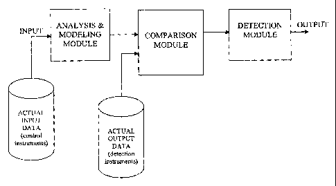
Figure 7 is a block diagram of a system corresponding to an embodiment of the
present
invention. An analysis module receives control instrument data from
infrastructure
12
CA 02596446 2007-08-08
sensors as input. A mathematical model processes the data and outputs an
estimated
behaviour for at least one detection instrument. A comparison module receives
the
estimated behaviour and compares it with actual output data (detection
instruments data)
stored in a database. A set of residuals corresponding to the difference
between the actual
data and the estimated behaviour is generated by the comparison module and
received by
a detection module. The detection module compares the residuals to a
predetermined
threshold and detects an anomaly when the threshold is exceeded. The anomaly
may be
in the form of an alarm or a flag, as described below. It should be understood
that the
mathematical model used to model the behaviour of at least one detection
instrument may
be a CCIM, DCIM, HST, Fuzzy-neural, Bayesian, or other known models, which are
known to a person skilled in the art.
Accessing and visualization of dam instrumentation/sensors data is available
for both the
past data stored in databases and the data that is measured in real-time as
time evolves.
The viewing capabilities extend from viewing a single sensor data in the form
of a table
or a chart to viewing multiple sensor data by simple drag and drop operation.
Furthermore, customized layouts of charts and/or tables for a group of sensors
of more
interest to dam safety operators can be designed and saved into the
application so that
each time by opening the layout the user would be able to see the data for all
those
sensors. Thus, the layouts help the dam safety operators to save a lot of time
by just one-
time loading of the layout of interest without requiring spending so much time
to open
the sensor data one-by-one.
Data validation and pre-processing/pre-filtering is performed in order to
clean up the
sensor data from irregularities and spikes as well as missing values. Such
irregularities
and spikes are quite common due to sensor noise, environmental disturbances,
and human
operator mistakes or miscalculations. Out of bound values, where the user
specifies the
upper and lower bounds, are getting detected and replaced by the interpolated
values.
Similarly, the missing values in the data are replaced by either some fixed
value that is
specified by the user or by interpolation.
For data analysis and modeling purposes, the data for all sensors should have
equal/uniform time-step. However, in almost all existing dam structures there
still exist
lots of manual measurements, as compared against the measurements that are
provided
13
CA 02596446 2007-08-08
by Automatic Data Acquisition Systems (ADAS). While in all ADAS systems it is
fairly
simple to adjust or set the reading frequency of the instruments, the manual
measurements are characterized with sparse and irregularly time spaced
readings. Thus,
for successful and meaningful analysis and modeling purposes, we first need to
generate
time-series with uniform time steps for all the available instrumentation data
of interest.
The present software solution can generate uniform time series from the raw
data with
any required time-step such as monthly, daily, hourly, etc., and any desirable
type of
interpolation techniques including zero-order hold, first-order hold, line
interpolation,
averaging, sinusoidal interpolation, just to name a few. Also we are able to
not only up-
sample the raw data using the interpolation techniques some of which are
mentioned
above, but also the raw data can be down-sampled in cases that the user wants
to have a
time-series with lower reading frequency than the one of the raw data.
There is provided real-time dam health monitoring by the primitive techniques
of bounds
checking for both the sensor data and its rate of change. Based on the a
priori knowledge
on the feasible bounds on a specific sensor and the feasible rate of change of
data for that
sensor, one can check the raw data against those bounds and evaluate the
health status of
that specific sensor. As a simple example consider the sensor data for
piezometers.
Practically, the piezometers data should never show negative values. Thus,
whenever a
negative value is seen in the data it means that there had been some anomaly
such as
calibration problem in piezometers.
The embodiments of the invention described above are intended to be exemplary
only.
The scope of the invention is therefore intended to be limited solely by the
scope of the
appended claims.
14