Note : Les descriptions sont présentées dans la langue officielle dans laquelle elles ont été soumises.
CA 02829617 2013-09-10
WO 2012/129654 PCT/CA2012/000272
MULTI-COMPONENT ELECTROMAGNETIC PROSPECTING APPARATUS AND
METHOD OF USE THEREOF
FIELD OF THE INVENTION
This invention relates to electromagnetic prospecting methods. More
particularly, this
invention relates to methods of electromagnetic prospecting for conductive
bodies.
BACKGROUND OF THE INVENTION
Controlled source electromagnetic (EM) systems have been used for many years
for
prospecting for minerals (Grant and West, 1965; Nabighian, 1991). In more
recent years,
they have also been used for groundwater investigations, environmental
investigations (Ward,
1990), the detection of unexploded ordnance (e.g., Billings et al., 2010) and
more recently in
agricultural mapping (Luck and Milner, 2009). Electromagnetic systems have
also been used
in resistivity logging tools (Wang et al., 2009; Davydycheva, 2010a; 2010b)
and in seafloor
controlled source electromagnetic (CSEM) systems (Chave and Cox, 1982;
Cheesman et al.,
1987; 1988; MacGregor and Sinha, 2000; Ellingsrud et al., 2002; and Constable
and Srnka,
2007).
These controlled source EM systems comprise a transmitter and a receiver. The
transmitter is generally a loop carrying a time varying current. According to
Ampere's law,
this current has a magnetic field that radiates away from the transmitter in
all directions,
including below the ground surface. If this field, called the primary field,
varies as a function
of time, then there is an electric field that circulates around the time
varying magnetic field. If
this electric field passes through a region of the subsurface that has a non-
zero electrical
conductivity, then the product of the electrical conductivity and the electric
field gives a
current density (Ohm's law). These currents induced in the ground are called
secondary
currents. The secondary currents have an associated secondary magnetic field
(Ampere's
law) which radiates everywhere, including above the surface of the earth,
where it can be
measured by a receiver coil. The receiver coil also measures the primary field
that comes
directly from the transmitter. Generally, there has to be some form of
communication or
timing link between the transmitter and the receiver so that the measured
field can be
1
CA 02829617 2013-09-10
WO 2012/129654 PCT/CA2012/000272
decomposed into a field that is similar in shape and timing (phase) to the
primary. This
component is called the "in-phase" response. Anything that is not in-phase can
be considered
the out-of-phase or "quadrature phase" component. The systems that have
transmitter current
waveforms that are sinusoidal are classified as frequency-domain systems, ones
with
waveforms that switch off suddenly in some manner are known as time-domain
systems.
Both time and frequency domain systems have in-phase and quadrature components
(Smith,
2001).
Systems have been designed to have the transmitters and receivers on the
ground and
mounted on aircraft. In some cases the transmitters and receivers are
connected to the
aircraft, in other cases the transmitter is attached to the aircraft and the
receiver towed by a
long cable behind the aircraft and housed in a "bird". There is an enormous
variety of EM
systems operating with different geometrical configurations and different
waveforms.
EM systems generally fall into two categories: profiling methods and large-
loop
methods (Frischknecht et al., 1991; Parasnis, 1991; Nabighian and Macnae,
1991). In the
profiling methods, the transmitters and receivers move together over the
volume to be
investigated with the transmitter and receiver a fixed distance apart. In some
cases, more than
one separation will be used to provide more data or to look to different
depths. The large-
loop methods generally have the transmitter in one location and the receiver
in multiple
locations. In some cases, multiple transmitter loop locations will be used to
provide more
data or to excite the earth at different locations or with a primary field
with different
directions. The receivers can be on the ground or airborne and the
transmitters can be
airborne or on the ground. Semi airborne methods have one subsystem (e.g. the
transmitter)
on the ground and the other in the air (Smith et al., 2001).
The Slingram or horizontal loop EM systems (Telford et al., 1976; Frischknecht
et al.,
1991) are a simple example of a profiling system. These systems generally use
a single
component transmitter and a single component receiver at a fixed separation.
The airborne
methods generally use a transmitter and receiver pair at a particular
separation. The early
airborne systems used one transmitter and one receiver (Davidson, US Patent
2652530).
Additional information about the geometry of the target in the ground was
obtained using two
pairs of transmitters and receivers, one pair coaxial, where the transmitter
and receiver coils
2
CA 02829617 2013-09-10
WO 2012/129654 PCT/CA2012/000272
are aligned so that their dipole direction (or normal vector) is pointed along
the direction of
flight and one pair coplanar, where the transmitter and receiver coils lie in
a common plane ¨
generally horizontal (Fraser, 1979; Fraser, US Patent 4367439). It was also
recognized that
using a single transmitter and multiple component receivers could also provide
extra
geometric information (Fraser, 1972; Arman, 1986; Best and Bremner, 1986; and
Smith and
Keating, 1996). Specifically, Fraser (1972) and Smith and Keating (1996)
showed that it was
possible to determine the depth, dip strike and offset of conductors with the
information from
multiple receiver components. As an extension to this concept, Hogg (1986)
proposed a
system with three component receivers and two component transmitters and
performed some
model studies to show that the multiple components provided a wealth of data
that could be
used to infer the depth and orientation of the subsurface conductor.
The large loop systems (Parasnis, 1991; Nabighian and Macnae, 1991) generally
have
the loops laid out horizontally. Multiple receiver positions are then
occupied; usually one
receiver is moved sequentially over the survey area, but occasionally one or
more receivers
can be moved in parallel. The strength of this configuration is that the large
loop has a strong
field that will penetrate to great depth and excite strong currents in
conductive zones. The
weakness of the large loop configuration is that the magnetic field vector at
any point in the
ground only points in one orientation. The electric field circulating around
the magnetic field
is also in one orientation. If there is no conductive pathway in this
orientation, then a
substantial current will not be induced. In the jargon of electromagnetic
prospecting, in this
case, the primary field is said to couple poorly to the conductor. If the
field is oriented so the
electric field is aligned with a conductive pathway, then the field couples
strongly to the
conductor. The magnetic field directly below a large loop is vertical, so this
primary field
will couple well to horizontal conductors. In order to couple well to a
vertical conductor, the
field must be horizontal, which is only true at some distance and some depth,
where the
primary fields are weak. One solution to this problem is to design a loop in
the shape of a
figure eight symbol (8) or infinity symbol (00), either in parallel (Spies
1975) or in series
(Brube et al., US Patent 7116107 B2). If there is some uncertainty as to the
orientation or
location of a conductor, a well designed survey will often include a number of
transmitter
positions to provide multiple coupling directions in a zone of interest. Each
additional large
3
CA 02829617 2013-09-10
WO 2012/129654 PCT/CA2012/000272
loop takes time to lay-out and thus increases the cost of the survey. Seismic
methods (Telford
el al, 1976) have developed the concept of arrays of receivers and
transmitters (seismic
sources) to reduce noise.
The ability to detect and discriminate extremely good conductors is very
important in
mineral exploration. This means that the highly conductive copper and nickel
ore deposits
can be discriminated from other less conductive bodies such as iron and zinc
deposits and
graphite and clay. One of the difficulties in doing this is that the response
from the highly
conductive body has a waveform that is identical to the waveform coming from
the
transmitter. This identical waveform is called an "in-phase" response or
signal as it has both
the same waveform and the same timing or phase as the transmitter (primary)
waveform.
Because the response is in-phase, special methods are required to identify
these
extremely conductive deposits. One method is to make the transmitter and
receiver a fixed
distance apart and then use a special "bucking coil" to cancel out the primary
field from the
transmitter (McLaughlin, et al., US Patent 3015060; McLaughlin et al, Canadian
Patent
684662). The bucking coil is usually smaller than the transmitter, closer to
the receiver and is
positioned and oriented so that the field from the transmitter and bucking
coil cancel at the
receiver. Whitton (Canadian Patent Application 2420806) proposed that the
transmitting,
receiving and bucking coils be concentric. For these types of systems to work
well, it is
necessary that the transmitter and bucking coil transmit exactly the same
waveform and that
the distances and orientation of all the coils do not change. These systems
are called rigid
boom systems and examples such as those described by Ruddock et al. (Canadian
Patent
667736) and Taylor and Shaw (Canadian Patent 680143) were attached to or towed
below
helicopters. A patent held by De Brie Perry and Gribble (Canadian Patent
653286) mounts a
pair of coaxial and a pair of coplanar transmitters a small distance below the
extremes of the
wing tips of a fixed-wing aircraft. The intention of their patent is to
minimize the relative
movement of the transmitter and receiver coils, so they are attempting to make
the system as
rigid as possible. Methods that orient the receiver so that it is null coupled
with the
transmitter (e.g. Davidson, US Patent 2652530; Ruddock and Brant, US Patent
2887650) will
also measure no primary field. These methods also rely on the geometry being
held rigid.
Bucking coils have been proposed for non-rigid systems (Puranen and Kahma, US
Patent
4
CA 02829617 2016-12-07
2741736), but never implemented successfully as it is labourious, time
consuming and costly
(Robinson, Canadian Patent 854344).
A second approach is to continually monitor the geometry of the transmitter
and
receiver (e.g. the lateral offset and the orientation) and then predict the
field from the
transmitter. This predicted field can be subtracted and the residual is the
field from the
extremely good conductor. Hefford et at. (2006) showed that the closer the
transmitter and
receiver are to each other, the more stringent the accuracy that the geometry
must be known.
This approach is used successfully with ground or borehole EM systems (West et
al., 1984;
Smith and Balch, 2000), but not with airborne systems due to the very
stringent accuracy
requirement.
A third approach, proposed by Zandee (Canadian Patent 1202676), suggested
cross
correlating a transient transmitter signal with the received signal to
decompose the response
into in-phase and quadrature components at a number of frequencies and to use
the very low
frequency in-phase signal to correct for relative motion of the transmitter
and receiver.
However, this system was never demonstrated to work in practice. Another
patent by Zandee
and Ros (Canadian Patent 1247195) suggested sending a primary compensation
signal to the
receiver down the tow cable.
A fourth approach is to use two transmitters with different orientations and
exploit the
fact that the field from these two transmitters has different amplitudes.
Cartier et al (US
patent 2623924; Canadian Patent 564361) proposed using a coaxial and a
coplanar coil pair.
The field from the former will be twice as big as the field from the latter,
so deviations from
this ratio should identify when there are excellent conductors proximal to the
electromagnetic
system. This system assumes that the receivers lie along an axial line defined
by the
orientation of the coaxial transmitter and that the orientation of the
receiver is such that the
direction of the coaxial coil is along the line from the transmitter and the
coplanar coil is
perpendicular to this and parallel to the coplanar transmitter.
The implementation of this system had the receiver towed behind an aircraft,
so the
correct geometry could only be ensured at times when the winds were very calm.
Cartier et al
(US patent 2623924; Canadian Patent 564361) argued that the response was
relatively
insensitive to the relative position of the transmitter and receiver; however,
they also proposed
5
CA 02829617 2016-12-07
that a servo system could rotate the transmitter coils so that the axis of the
coaxial coil was
always pointing towards the receiver. A variation of this approach was taught
by Shaw and
Taylor (US Patent 2955250), who added an additional coil in the same
orientation as one of
the other coils, but transmitted a signal at a different frequency. A
subsequent invention by
Shaw and Taylor (US Patent 2955251) suggested that the relative position
between the
receiver and transmitter be guided by a modulated beam of light and controlled
by fins on the
transmitter and/or receiver.
Other methods of airborne electromagnetic systems that are not rigid, avoid
the
measurement of the in-phase response. Robinson (Canadian Patent 854344),
suggests
measuring the field in quadrature with the currents in the transmitter and the
aircraft. Time
domain systems (Barringer, Canadian Patent 662184; Kamenetsky et al., Canadian
Patent
889478) that measure in the off-time are essentially measuring the quadrature
field (Smith,
2001). Other approaches measure the total phase difference between an
operating frequency
and a lower frequency (Puranen and Kahma, US Patent 2642477) or differences in
the
response in two receivers when the transmitter radiates a rotary field
(Hedstrom and Tegholm,
US Patent 2794949). These systems are not sensitive to extremely conductive
bodies.
Another approach taught by Seigel (US Patent 2903642) measures the in-phase
distortion in the angle of the total field measured from two primary fields.
However, this
method is also insensitive to extremely good conductors, as the distortion of
the in-phase
response from the extremely good conductor will essentially be identical at
both frequencies.
Puranen (US Patent 2931973) teaches a method that uses two orthogonal
transmitters and two
orthogonal receivers and measures the in-phase and quardature components. An
airborne
method described by McLaughlin et al. (US Patent 3014176) proposes a single
transmitter
and receiver pair, a novel bird for controlling the geometry, a signal from
the transmitter to
cancel the receiver signal and measuring the quadrature component.
An invention taught by Nilsson (US Patent 4492924) suggested measuring the
electric
field, which, to the knowledge of the inventor, has not yet been successfully
commercialized
in an airborne EM system. Ronka (US Patent 3042857) suggested an airborne
system
comprising two coaxial (or coplanar) single-component transmitters with
moments with
opposite sign and magnitudes adjusted so that changes in geometry will result
in an increase
6
CA 02829617 2016-12-07
from one transmitter that nullifies the decrease from the other transmitter.
The preferred
embodiment suggests a three-axis receiver, a configuration that was not used
in practice in an
airborne electromagnetic system until the mid 1990s. Dzwinel (Canadian Patent
1188363)
teaches a method that uses a single-component transmitter and a three-
component receiver
towed below the transmitter. The patent described here introduces the use of
non-rigid,
separated three-component transmitters and receivers in the electromagnetic
system.
More recent patents relate to other innovations. One group proposes the use of
helicopters and controlling transmitter-receiver geometry (Taylor, Canadian
Patent 2187952;
Kremer, Canadian Patent 2232105; Klinkert, Canadian Patent Application
2564183), but not
specifically for the purposes of detecting extremely conductive bodies.
Another patent
suggests towing a small aircraft behind the aircraft (Klinkert, Canadian
Patent 2315781).
Morrison et al. in Canadian Patent Application 2450155 have designed a system
with a large
loop towed below an aircraft, but in the preferred embodiment, the aircraft is
a helicopter.
Another helicopter towed system comprising a large loop and a large minimum or
null
coupled receiver is described by Miles et al. in Canadian Patent Application
2584037 and US
Patent 7646201.
Multi-component transmitters and receivers are used in other fields of
investigation.
In the aerospace engineering and medical instrumentation fields, three-
component co-located
orthogonal dipoles and three component co-located orthogonal dipoles are used
to accurately
track and determine the relative position of objects (Knipers, US Patent
3,868,656; Raab, US
Patent 4054881; Raab et al., 1979; Anderson, US Patent 7,715,898; Schechter,
US Patent
Publication No. 2008/0309326). These systems are currently being used in a
variety of
applications. It has been recognized that the results provided by these
instruments are
perturbed by nearby conductive material (e.g. Jascob et al., US Patent
6636757; Anderson,
US Patent Publication 2006/0154604; Khalfin and Jones, Canadian Patent
2388328). US
Patent Publication No. 2010/0168556 provides a method for tracking a medical
device where
an electromagnetic error correction tool is employed to correct for local
metal distortion
effects. Other more complex systems have been developed subsequently (e.g.
Anderson, US
Patent 7015859 B2).
7
CA 02829617 2016-12-07
In the field of unexploded ordnance (UXO) detection, arrays of multiple
transmitters
and receivers are now being employed. The UXO detection instruments have the
transmitters
and receivers together in one housing that moves across the ground so they are
essentially
profiling instruments, housing the transmitters and receivers in one unit and
intending to
identify the UXO in a single pass over the ground. Generally, these UXO
detection systems
use an array of multiple transmitters and receivers arranged in a fixed-
geometry grid (Bell et
al., 2008) or a gradient measurement (e.g. Billings et al., 2010). Fan et al.
(2010) have also
recently proposed the use of multiple transmitters to direct the propagation
direction of a field.
The ALLTEM system (Wright et al., 2006) uses a three-component transmitter and
measures the vertical field response; the horizontal fields are all sensed by
measuring specific
gradients ¨ primarily the vertical gradients (Asch et al., 2009; 2010). The
reason for the
emphasis on gradient measurements is because the sensors are very close to the
transmitters,
so measuring the gradient is required to cancel the strong primary field. In
addition to
measuring gradients, other techniques are necessary to reduce the impact of
the primary field
(Asch et al., 2008). One of the advantages of the ALLTEM (Wright et al., 2005)
is its ability
to measure the on-time response; West et al. (1984) demonstrate that this
allows identification
of highly conductive electromagnetic responders or ferrous objects (magnetic
responders).
The ability to identify these on-time responses requires that the geometry is
fixed or known.
This is true for the ALLTEM system. The multiple component measurements in the
ALLTEM system are to provide additional geometric information about the
geometry of the
UXO.
A UXO system described by Zhang et al. (2010) uses a single component
transmitter
and a multiplicity of three-component receivers. Another UXO profiling system,
named BUD
(Smith et al., 2007; Gasperikova et al., 2008, Morrison and Gasperikova, US
Patent
Publication No. 2009/0219027), uses a three-component transmitter and eight
pairs of
differenced receivers (16 vertical dipoles) arranged in a fixed geometry
array. Another
system, the AOL (Snyder and George, 2006; Snyder et al., 2008) used a three-
component
transmitter and an array of three component receivers inside the horizontal
transmitter loop.
The Geonics UXO system EM63-3D-MK2 also used an orthogonal three-component
receiver
and an orthogonal three-component transmitter. In all cases, the UXO systems
have the
receivers rigidly connected to the transmitters. In addition, compared with
the size of the
8
CA 02829617 2016-12-07
targets and the size and position of the receivers, these UXO transmitters
could not be
considered as dipoles.
Three-component receivers have been taught in US Patent Publication No.
2010/0244843, filed by Kuzmin, where first and second sensor systems employing
three-axis
receivers are employed for measuring naturally occurring magnetic fields,
where parameters
are calculated that are independent of the rotation of the first or sensor
systems. Kuzmin also
teaches using the disclosed three-component receiver as part of a system that
uses a single
axis transmitter to generate artificial magnetic fields.
US Patent No. 4,628,266, issued to Dzwinel, discloses an electromagnetic
prospecting
system in which a transmitting system, suspended vertically from a helicopter,
is adapted to
radiate electromagnetic fields of many different frequencies and many
different orientations
controlled automatically. The transmitting operation is carried out over
several hundred
combinations of transmitting system characteristics: helicopter altitude,
electromagnetic field
frequency and transmitter loop inclination and direction. A receiving system,
suspended
vertically from the transmitting system, is adapted to detect signals of three
orthogonal
components of electromagnetic deviations as a function of helicopter altitude,
frequency,
transmitter loop orientation and receiver antenna orientation. A processing
system is provided
to store and process an enormous volume of data directly into probability
levels of
hydrocarbon presence or absence over the area explored.
Three-component transmitter and receivers have also been used in the triaxial
induction tools used in the hydrocarbon exploration industry. These tools
contain the
transmitters and receivers a fixed distance from each other (Wang et al.,
2009; Davydycheva,
2010a; 2010b) and the tool is moved up and down a borehole to measure the
anisotropy of the
resistivity of the sedimentary formations, any invasion zones, or any faults
that make the
geometry three dimensional. As the transmitters and receivers move as a single
entity down
the hole, these instruments are essentially acquiring a single profile down
the borehole.
Unfortunately, the aforementioned systems for detecting extremely good
conductors
are limited by their requirement for maintaining and controlling a fixed
spatial relationship
between the transmitter and receiver and often lack sensitivity in detecting
highly conductive
9
CA 02829617 2016-12-07
bodies. A system with a three component transmitter and a three component
receiver removes
this limitation.
Also, the profiling methods used for EM prospecting are limited in their depth
penetration and the large loop methods require that the coupling of the
transmitter to the target
in the subsurface be known. Accordingly, there remains a need for a versatile
and sensitive
electromagnetic prospecting system with improved sensitivity and
directionality in locating
conductive bodies.
SUMMARY OF THE INVENTION
Embodiments provided herein utilize a transmitter for electromagnetic
prospecting
comprising three co-located dipoles where no two dipoles are on the same plane
(non-
coplanar) and ideally are close to orthogonal. For brevity this transmitter
will be termed a
"three-component transmitter". This three-component transmitter can couple to
any target at
any orientation in the subsurface. In selected embodiments, by combining the
response
detected from one or more transmitters over multiple locations in a post-
processing step, an
array of multiple transmitters and optionally multiple receivers can be formed
for achieving
an improvement in the signal to noise ratio and the potential depth that the
system could
sense. Advantageously, such arrays of multiple three-component transmitters
can be used to
effectively focus the electromagnetic signal at a particular location for
increased sensitivity.
Accordingly, in a first aspect, there is provided a method of electromagnetic
sensing
comprising the steps of: a) driving each co-located transmitter of a three-
component electric or
magnetic dipole transmitter provided at a transmitter location to generate
three multiplexed
electromagnetic fields, and, while driving each transmitter of said three-
component transmitter,
measuring signals with each receiver of a three-component receiver provided at
a receiver location,
thereby obtaining nine received signals; b) repeating step (a) for a plurality
of different transmitter
locations, different receiver locations, or a combination thereof, thereby
obtaining a set of received
signals; c) evaluating said set of received signals to assess the presence of
a conductive body.
According to another aspect of the invention, there is provided a method of
electromagnetic sensing comprising the steps of a) driving each co-located
transmitter of a
three-component transmitter provided at a transmitter location to generate
three multiplexed
CA 02829617 2016-12-07
electromagnetic fields, and, while driving each transmitter of the three-
component transmitter,
measuring signals with each receiver of a three-component receiver provided at
a receiver
location, thereby obtaining nine received signals; b) repeating step (a) for a
plurality of
different transmitter locations, different receiver locations, or a
combination thereof, thereby
obtaining a set of received signals; c) selecting a sensing direction and a
sensing position; d)
determining a set of transmitter weights, such that wherein the weights are
multiplied by
electromagnetic fields produced at the sensing position by each transmitter at
each transmitter
location, and wherein a resulting set of weighted electromagnetic fields are
summed over
each transmitter location, a summed weighted field is enhanced in the sensing
direction at the
sensing position, and substantially suppressed at other positions and
directions; e) multiplying
each signal of the set of received signals by a corresponding transmitter
weight, wherein, for a
given three-component receiver, the corresponding transmitter weight is a
weight determined
in step (d)
1 Oa
CA 02829617 2016-12-07
for a transmitter that was active when a signal was recorded with the given
three-component
receiver; f) summing a resulting set of weighted signals to obtain a focused
signal; and g)
inferring a presence or absence of a conductive body at the sensing position
according to a
strength of the focused signal.
The method may further comprise the steps of: h) selecting one or more of an
additional sensing direction and an additional sensing position; and i)
repeating steps d) to g),
and may optionally further comprise repeating steps h) and i) one or more
times to scan one or
more of a spatial and angular region.
A three-component transmitter may be provided to one or more of the different
transmitter locations by translating a single three-component transmitter, or
alternatively
a physically separate three-component transmitter may be provided at one or
more of the
different transmitter locations. Similarly, a three-component receiver is
provided to one or
more of the different receiver locations by translating a single three-
component receiver, or
alternatively a physically separate three-component receiver may be provided
at one or more
of the different receiver locations. Each three-component receiver may
comprise three dipole
receivers suitably arranged to be capable of detecting an electromagnetic
field in any
direction. The transmitter and receiver dipoles can be magnetic or
electromagnetic dipoles.
The method may further comprise the step of determining, based on the set of
signals,
a location from which a secondary electromagnetic field was generated.
The method may further comprise the step of calculating a reference signal
produced
by a theoretical conductive body located at the sensing position, and
comparing the reference
signal with the focused signal. The step of comparing the reference signal
with the focused
signal may comprise cross-correlating the reference signal with the focused
signal.
The multiplexed electromagnetic fields may be multiplexed in the time domain
or the
frequency domain.
In another aspect, there is provided a method of electromagnetic sensing
comprising
the steps of: a) driving each transmitter of a three-component co-located
transmitter provided
at a transmitter location to generate three multiplexed electromagnetic
fields, and, while
driving each transmitter of the three-component transmitter, measuring signals
with each
receiver of a three-component receiver provided at a receiver location,
thereby obtaining nine
11
CA 02829617 2016-12-07
received signals; b) repeating step (a) for a plurality of different
transmitter locations,
different receiver locations, or a combination thereof, thereby obtaining a
set of received
signals; c) forming an a set of equations relating the set of received signals
to the properties of
one or more subsurface conductive body in response to primary electromagnetic
fields
transmitted by the three-component transmitter; and d) solving theses
equations using any
well-known non-linear inversion method to obtain locations of the one or more
subsurface
conductive bodies. Examples of non-linear algorithms that are familiar to
those experienced in
the art are described by Marquardt (1963) and Gill and Murray (1978).
In yet another aspect, there is provided a method of detecting the presence of
a
conductive body, the method comprising the steps of: providing a three-
component co-located
transmitter and a three-component receiver, driving each transmitter of the
three-component
transmitter to generate three multiplexed electromagnetic fields; detecting
the three
multiplexed electromagnetic fields with each receiver of the three-component
receiver,
thereby obtaining measured values for nine electromagnetic field components;
generating
equations that relate the nine electromagnetic measurements to the position
and orientation of
the three-component transmitter; solving the equations using well-known non-
linear inversion
techniques to estimate a position and orientation of the three-component
transmitter relative to
the three-component receiver; employing the position and orientation to
calculate predicted
values of the nine electromagnetic field components, and calculating a
residual
electromagnetic field by subtracting predicted values from the measured
values; and inferring
a presence of a conductor based on a non-zero residual electromagnetic field.
The three-component transmitter may comprise three non-coplanar dipole
transmitters
and the three-component receiver comprises three non-coplanar dipole
receivers. The step of
inverting the equations may comprise performing any well known non-linear
iterative
method, for example those cited by Marquardt (1963) and Gill and Murray
(1978).
The three-component transmitter and the three-component receiver may be
separated
by an initially unknown distance.
The multiplexed electromagnetic fields may be multiplexed in the time domain
or the
frequency domain.
12
CA 02829617 2016-12-07
In another aspect, there is provided a method of detecting the presence of a
conductive
body, the method comprising the steps of: providing a three co-located
transmitter and a
three-component receiver, driving each transmitter of the three-component
transmitter to
generate three multiplexed electromagnetic fields; detecting the three
multiplexed
electromagnetic fields with each receiver of the three-component receiver;
generating a set of
equations relating vector or scalar products derived from the three
multiplexed
electromagnetic fields, said products and equations are invariant to rotation
of the receiver;
solving the equations to determine a position of the three-component
transmitter relative to
the three-component receiver; generating a linear combination of the three-
component fields
that would have fields that are equivalent to the fields from a rotated three-
component
transmitter such that one dipole of the three-component transmitter is
directed along an axis
passing through the location of the three-component transmitter and the three-
component
receiver; and inferring a presence of a conductive body based on a non-zero
value of one or
more vector or scalar products of said linearly combined fields from the
rotated transmitter, or
a combination of vector and scalar products, that are expected to be zero in
absence of the
conductive body.
The three-component transmitter may comprise three non-coplanar dipole
transmitters
and the three-component receiver comprises three non-coplanar dipole
receivers. The
multiplexed electromagnetic fields may be mutually orthogonal at a location of
the three-
component receiver.
The three-component transmitter and the three-component receiver may be
separated
by an initially unknown distance.
The multiplexed electromagnetic fields may be multiplexed in a time domain or
a frequency domain.
A further understanding of the functional and advantageous aspects of the
invention
can be realized by reference to the following detailed description and
drawings.
BRIEF DESCRIPTION OF THE DRAWINGS
Preferred embodiments of the invention will now be described, by way of
example
only, with reference to the drawings, in which:
13
CA 02829617 2016-12-07
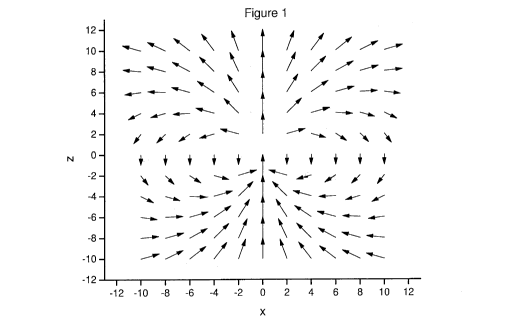
Figure 1 illustrates the magnetic field produced by a magnetic dipole at the
origin
directed up the z axis m=(0,0,1) (the magnitude of each vector has been
multiplied by 471r3/ 0
to increase the magnitude of the arrows distant from the dipole).
Figure 2 plots the vector magnetic fields at a subsurface point (-10,-10,-10)
from a
transmitter comprising three dipoles all co-located at the origin. The fields
A, B and C are
from transmitters in the X, Y and Z directions respectively.
Figure 3 plots the vectors at the same point as in Figure 2 when the three-
component
transmitter is rotated so that one axis (in this case the z axis) is aligned
with the vector joining
the subsurface point to the transmitter, where the dipole along the rotated z
axis (ZR) has a
field (CR) that is coaxial (also points along the axial vector); the rotated X
axis (XR), now
pointing down and in, has a field (AR) that is anti-parallel (pointing up and
out); and the
rotated Y axis (YR), now pointing left and in, has a field (BR) that is anti-
parallel, pointing
right and out.
Figure 4 illustrates the effect of multiplying the magnitude of the X
transmitter by -
0.5 and multiplying the Y and Z transmitters by 0.5 and then adding the
resulting fields,
where the resultant field at the point (-10, -10, -10) is purely in the x
direction. This is
equivalent to a similar linear combination of the fields A, B and C at the
same point
associated with the X, Y and Z component transmitters, and as a result, linear
combinations of
transmitters can thus direct the field at any point.
Figure 5 illustrates the outcome when an array of multiple transmitters, all
directed to
give an x-directed field at (0, -10, -4) are summed together, where the field
at this point
(circled) is even stronger than it would be for one three-component
transmitter location (note
however that the field at other locations is in different orientations and can
also be stronger).
Figure 6 illustrates how a linear combination of the fields from all the
transmitter
locations adjusted to give a strong x-directed field at the location of
interest (circled) and
weak fields elsewhere (note that the relative sizes of the arrows depicting
the transmitter
fields have been adjusted in proportion to their strength).
Figure 7 illustrates a matrix equation that is employed to calculate the
transmitter
weights.
14
CA 02829617 2016-12-07
Figure 8 shows a current induced in the ground in a conductive body at
location (0,-
10,-4) oriented such that the dipole that represents the field points along
the x axis direction,
where the arrow representing this dipole at this location has been circled.
The field at the
surface (z=0) from this dipole has the vector components shown. A receiver
array with
multiple receivers laid out at the locations of the arrows would measure the
shown response.
Figure 9 is a flow chart illustrating a method of detecting the presence of a
conductive
body using three-component transmitters.
Figure 10 is a system level diagram showing the components of a system that
may be
employed for the detection of a conductive body using an array of three-
component
transmitters.
Figure 11 schematically illustrates an embodiment of a computing system for
use in
the system shown in Figure 9.
Figure 12 is a flow chart illustrating a method of detecting the presence of a
conductive body using a three-component transmitter and a three-component
receiver
separated by an arbitrary distance, where the method involves subtracting a
calculated
transmitter field from the measured signal at the receiver.
Figure 13 is a flow chart illustrating another method of detecting the
presence of a
conductive body using a three-component transmitter and a three-component
receiver
separated by an arbitrary distance, where the method involves the solution of
a set of invariant
equations.
Figure 14 plots the changing geometric relationship between a three-component
transmitter and a three-component receiver as a function of distance along a
profile, where the
offset of the receiver from the transmitter is given by the x, y and z values
and the orientation
of the receiver is defined by the roll, pitch and yaw in the bottom three
panels.
Figure 15 plots the rotational invariants of the total field (from the
transmitter and the
anomalous body) at the receiver, where, in this case, the transmitter if
oriented with its z axis
vertical. Most of the variation observed in the invariants is due to changes
in the x, y and z
offset (the invariants have units of (A/m)2).
Figure 16 plots the rotational invariants of the total field (from the
transmitter and the
anomalous body) at the receiver, where, in this case, the transmitter is
rotated so that its z axis
CA 02829617 2016-12-07
is oriented along the vector joining the transmitter and receiver. As shown in
the Figure,
when 4j the 1-4=11.1= terms are zero, except where there is a secondary
response, in which case
the term shows a non-zero anomalous response. In the case when the two vectors
in the dot
product are the same (=j) there is not an anomalous response (the invariants
have units of
(A/m)).
Figure 17 plots the value of equations 28 and 29 involving combinations of the
1-11-H1
terms, where these combinations now have a zero response away from the
conductor and an
anomalous response at the conductor.
DETAILED DESCRIPTION OF THE INVENTION
As required, embodiments of the present invention are disclosed herein.
However, the
disclosed embodiments are merely exemplary, and it should be understood that
the invention
may be embodied in many various and alternative forms. The Figures are not to
scale and
some features may be exaggerated or minimized to show details of particular
elements while
related elements may have been eliminated to prevent obscuring novel aspects.
Therefore,
specific structural and functional details disclosed herein are not to be
interpreted as limiting
but merely as a basis for the claims and as a representative basis for
teaching one skilled in
the art to variously employ the present invention. For purposes of teaching
and not limitation,
the illustrated embodiments are directed to a multi-component electromagnetic
prospecting
apparatus and methods of detecting subsurface conductive bodies.
As used herein, the ten-ns, "comprises" and "comprising" are to be construed
as being
inclusive and open ended, and not exclusive. Specifically, when used in this
specification
including claims, the terms, "comprises" and "comprising" and variations
thereof mean the
specified features, steps or components are included. These terms are not to
be interpreted to
exclude the presence of other features, steps or components.
As used herein, the term "exemplary" means "serving as an example, instance,
or
illustration," and should not necessarily be construed as preferred or
advantageous over other
configurations disclosed herein.
16
CA 02829617 2016-12-07
As used herein, the terms "about" and "approximately", when used in
conjunction
with ranges of dimensions of particles, compositions of mixtures or other
physical properties
or characteristics, are meant to cover slight variations that may exist in the
upper and lower
limits of the ranges of dimensions so as to not exclude embodiments where on
average most
of the dimensions are satisfied but where statistically dimensions may exist
outside this
region. It is not the intention to exclude embodiments such as these from the
present
invention.
As used herein, the term "aircraft" is intended to encompass any flying
vehicle,
including, but non-limited to, fixed-wing aircraft, rotary-wing (helicopter)
aircraft, blimps,
airships, unmanned airborne vehicles, balloons, and the like. When
instrumentation is
"carried by an aircraft" it can be attached to the aircraft or towed.
Embodiments disclosed herein provide improved electromagnetic prospecting
apparatus and methods for exploring a volume of material beneath the surface
of the earth,
and identifying conductive bodies. Unlike known solutions, the present
embodiments employ
a transmitter that comprises three co-located dipoles and/or receivers, where
said three-
component transmitter and receivers may be rotated (or subjected to equivalent
operations)
virtually via mathematical rather than physical operations.
The key feature of said three-component transmitter is that the exciting field
from the
transmitter is able to induce currents in a target body that has an arbitrary
location and
orientation.
In selected embodiments, an array of three-component transmitters is employed
to
generate a localized electromagnetic field at a specific orientation at a
selected subsurface
location. This will induce a secondary field at this specific location.
Advantageously, the
utilization of multiple transmitter locations focuses the field and improves
the strength of the
secondary field generated at a given subsurface location. Furthermore, by
using three-
component receivers at multiple locations, the signal-to-noise ratio of the
measured signal
may be further increased.
In another embodiment, a three-component dipole transmitter is employed in
combination with a simple (non-gradient) three-component receiver dipole that
is not a fixed
(or precisely known) distance, but is separated from the transmitter by a
variable distance. As
17
CA 02829617 2016-12-07
shown below, when both the transmitter and receiver possess three components,
the response
of highly conductive bodies can be detected without knowing a-priori the
precise geometric
relation of the transmitter to the receiver, or holding the relative geometry
between the
transmitters and receivers constant. It is instead sufficient to maintain the
relative orientation
of each component with respect to the other two components in the transmitter
(or receiver).
The embodiments provided below overcome the difficulty of limited variety in
coupling
direction, while retaining the large signal strengths associated with a large
loop survey.
Prior to describing various embodiments in detail, a heuristic introduction is
provided
in order to explain the principles of electromagnetic prospecting, and the
relative advantages
afforded by solutions provided herein. For the purposes of teaching and not
limitation, the
examples provided below assume that the electromagnetic transmitters and
receivers are
magnetic dipoles. Generally speaking, embodiments disclosed herein involve the
use of dipole
transmitters and receivers for the generation of electromagnetic fields and
the detection of
secondary electromagnetic fields that are remotely produced by conductive
bodies. A
magnetic dipole is generated by an antenna that typically comprises one or
more loops of a
conductive coil. An electric dipole is a short conductor that injects an
electric field into the
medium.
The formula for the magnetic field vector H(r) at a location r=(x,y,z) from a
magnetic
dipole located at the origin (0,0,0) is given by the following equation
(Billings et al., 2010,
after correction)
H (r) = _______________________ (3 (in' = r')/-1 - (1)
4 n-r2.
where r is the scalar distance from the dipole to the observation location (x2
ty2 +z2 )I/2, m is
the magnitude of the dipole moment of the transmitter, m' is the unit-vector
orientation of the
dipole moment, E' is the unit vector from the dipole to the observation
location, and the'
symbol denotes a unit vector. The formula for the electric field from an
electric dipole is
identical except M is the electric dipole moment and there is a dielectric
permittivity on the
bottom line of the term out the front. If the magnetic dipole vector is
oriented up the z axis,
then the unit-vector orientation is m'=(0,0,1). In the case when the
observation point is
aligned along the axis of the transmitter dipole, then m'---- r' and m' r' =
1. This means that
18
CA 02829617 2016-12-07
(r) = _________________________________ (2 mil (2)
4r.rra
and the magnetic field is in the m' direction. In the case when the
observation point is in the
plane that is normal to the dipole orientation and contains the dipole, then
m' and r' are
perpendicular and m'= r'= 0. This means that
11(r) = ___ (m') (3)
(3)
45rr2
and once again the magnetic field is in the m' direction, although in this
case it is pointing in
the opposite (negative) direction. The magnitude is half that when the
observation point is on
the axis (for the same value of r). When the observation point is away from
these two special
locations, the orientation of the field is a linear combination of the r' and
m' directions.
The magnetic field vectors of a dipole located at the origin and oriented up
the z axis is
illustrated in Figure 1. The lengths of the arrows have been multiplied by
47rr3 so that the
vectors more distant from the dipole can be seen. The field of a dipole is
axially symmetric
about the z axis, so this image should be rotated about the z axis to create
the field in three
dimensions. The locations where the field contains only a vertical component
is when it is up
(on the z axis) and down (on the x-y plane where z=0). In the latter case, the
plane where the
field is pointing down will be called the normal plane, as it is the plane
that contains the
dipole and is normal to the dipole orientation. At the origin the dipole field
is singular.
Elsewhere, the dipole field contains a non-vertical component.
To take advantage of these properties of the dipole field, one may consider
the
situation where a three-component transmitter excites subsurface materials
located beneath
the ground. Figure 2 shows a transmitter, which without loss of generality,
all three dipoles
are co-located at the origin. The field at a location in the subsurface at (-
10, -10, -10) is
shown with the three arrows A, B, and C. The field designated A, originates
from the field
produced by the transmitter dipole aligned along the x axis; field B is from
they-axis aligned
transmitter dipole and field C is from the z-axis aligned transmitter dipole.
Note that these
fields are not orthogonal. Moving the location in the ground produces other
fields that can be
more or less orthogonal.
The transmitter shown in Figure 2 has the coils rigidly aligned in an
orthogonal set.
The coil set can alternatively be rotated so that one of the axes lies along
the axial vector from
19
CA 02829617 2016-12-07
the subsurface point to the transmitter. Figure 3 illustrates the case where
the x axis is first
rotated by 45 degrees around the z axis towards they axis, and then the z axis
is rotated
around they axis 54.7 degrees towards the horizontal plane. This rotated
transmitter set is
designated XR YR ZR and importantly, the three fields from these transmitters
AR, BR and CR
now form an orthogonal set (as can be seen in Figure 3).
The reason for the orthogonality of the remote transmitted field is that one
dipole (in
this case the ZR dipole) is aligned along the axial vector, so any field along
the axis from this
dipole will also be aligned along the axial vector. The XR and YR transmitters
are orthogonal
to the axial vector and orthogonal to each other. The axial vector lies at the
intersection of
both the normal planes of the XR and YR transmitters, so that the field along
the axial vector
from these transmitters is anti-parallel to each transmitter dipole and hence
also orthogonal to
the axial vector and each other.
As a result, the subsurface field on the axial vector now comprises an
orthogonal set
and from basic vector theory, a field at any arbitrary orientation can be
constructed as a linear
combination of this orthogonal set. The orthogonal set was obtained by
rotating the
transmitter set, but the same effect can be mathematically obtained by
performing a virtual
rotation by summing a linear combination of the transmitters shown in Figure
2. For
example, the ZR = (0.5773, 0.5773, 0.5773) = 0.5773 X + 0.5773 Y + 0.5773 Z.
Similarly, as it is known that a linear combination of the transmitter dipole
can be used
- 20 to construct an orthogonal set at the subsurface point, it also
follows that a linear combination
of the original fields A, B and C can be used to construct an orthogonal set.
As an example of
this result, if it is desired to construct a field that points along the x
(1,0,0) direction, one can
solve for the coefficients xl, x2, x3 that satisfy the equation
(A1\4- (13 1') 1) (1\
Xi A2 X2 B2 1-- X3 C2 = 0 , (4)
Asi \B3, C3 \.0/
where A, are the individual elements of the field A due to the X transmitter
(similarly for B,
and C,).
In the case of Figure 2, one can solve this equation and obtain (x1,x2,x3)=(-
0.5, 0.5,
0.5). Accordingly, by multiplying the original moments of the X, Y and Z
directed
transmitters by these three coefficient weights directly and summing, the
resultant three fields
CA 02829617 2016-12-07
will yield the primary field, in the desired (x) direction (Figure 4). Other
linear combinations
of the transmitter can give the other cardinal directions, and indeed any
arbitrary direction.
This linear combination of orthogonal transmitter dipoles to give a directed
vector in the
subsurface will henceforth be referred to as a "directed transmitter".
As shown above, one directed transmitter will give a directed primary field at
a
subsurface location. If multiple transmitters are provided and directed to
give the same
primary directed field, then the strength of the field at the subsurface
location can be
increased in proportion to the number of transmitters used. As shown in Figure
5, multiple
transmitters are all directed to generate a primary field in the x direction
at location (0 -10 -4),
shown by the circled vector in the Figure. Notice that the field at this
location is indeed
horizontal, as desired. It is noted, however, that the fields at shallower
depths are larger, as a
result of the fact that the field from a dipole decreases rapidly as a
function of depth.
Referring now to Figure 6, an exemplary illustration is provided, in which all
the
transmitter dipoles reside on the plane z=0. The length of each dipole is
proportional to the
weight applied to each dipole (the relative magnitude of the excitation
current provided to
each dipole). The subsurface field of this array is shown at a 3D grid of
representative points
below the surface. As prescribed, the transmitter dipole amplitudes are
selected such that the
only significant field is the desired horizontal field at location (0, -10, -
4), again, as shown by
the circled vector in the Figure. In the present example, the dipole
amplitudes and transmitter
rotations have been selected so that all other fields are suppressed by a
factor of
approximately one thousand (accordingly, these much smaller vectors are not
visible in the
Figure). A different linear combination of the fields produced by the
transmitter dipoles could
be used to focus the electromagnetic energy on any other desired location at
any other desired
orientation in the volume of interest.
In the exemplary case shown in Figure 6, a large number of three-component
transmitters were employed. I Iowever, if fewer transmitters are included in
the array, it is
expected that the ability to focus the field and/or suppress fields in other
locations would be
reduced. Furthermore, although the example illustrated in Figure 6 relates to
a sensing
position located at the edge of the volume below the transmitter array, it is
expected that
improved field focusing and non-local field suppression would be achieved for
a sensing
21
CA 02829617 2016-12-07
position located beneath the center of the transmitter array. Preferably, the
transmitters should
be located such that their spacing is comparable or smaller than the size of
the targets being
sought and the volume being investigated is within a projection of the
transmitter array plane.
A receiver is provided to sense the secondary field radiated by a conductive
feature
located at the sensing location. The signal-to-noise and position sensing
ability of the system
may be further improved by employing an array of receivers. Further
improvements will
come with the use of three-component receivers, as shown in Figure 8.
For example, using the same subsurface point as in the previous example, one
may
assume that a conductive body exists at that point and currents could flow in
a vertical plane
parallel to the y-z plane. A dipole representing these currents would be
directed along the x
axis (shown by the circled arrow in Figure 8). The secondary fields from a
dipole at this
position would have a three-component response as shown at each receiver
location in the
plane (the lengths of the arrows shown at the receivers are proportional to
the lengths of each
individual component that would be measured). In this figure, it is assumed
that the receivers
that make up the receiver array are all at the same locations as the
transmitters in Figures 5
and 6 (which they need not be).
It is expected that the use of a focused transmitter arrays and focused
receiver arrays
will enable the directed investigation of the subsurface at specific
locations. The strong signal
enhancement and noise rejection of the transmitter and receiver arrays will
enable sharper
resolution images and greater depth of investigation. In one embodiment, the
fields detected
by the array of three-component receivers may be employed to locate the
position from which
the secondary field originated, and to compare this sensing location to the
location where the
transmitted field was focused. This comparison can be useful in confirming
that the detected
field represents a conductive body.
In one embodiment, aspects of the preceding examples are utilized to achieve
an
increase in sensitivity. As illustrated in the flow chart provided in Figure
9, one or more three-
component transmitters are employed to sequentially generate primary
electromagnetic fields
that probe a spatial region of interest. In step 100, each transmitter of the
three-component
transmitter is separately and sequentially excited. Multiple transmitters can
transmit
simultaneously if multiplexed in the frequency domain as described below. In
step 110, a
22
CA 02829617 2016-12-07
three-component receiver is provided to individually detect, with each
receiver of the three-
component receiver, secondary electromagnetic fields produced in response to
the
electromagnetic fields from the three transmitter dipoles. Accordingly, nine
separate signals
are obtained by the three-component receiver. This process is repeated, as
shown at step 120,
for multiple transmitter locations to obtain receiver signals, for each
component in the three-
component receiver, that are obtained for each transmitter of the three-
component transmitter
at multiple locations near the region to the region of interest.
The principle illustrated graphically in Figure 6 and mathematically in Figure
7 may
then be employed to post-process the receiver signal data in order to obtain a
focused signal at
a selected position. This is because the signal response detected with the
three-component
receiver varies in a linear manner with the transmitter signal and a linear
combination of
transmitter dipole strengths may be employed as a post-processing step to
effectively focus
the transmitter field at a specific location and orientation. As shown in step
130, the post-
processing is performed by determining the weights associated with each
transmitter that may
be multiplied with the corresponding individual receiver signals such that the
sum over all the
weighted transmitters is used to obtain a signal at each receiver position.
This sum over
transmitters is intended to provide enhanced directional sensitivity to a
selected subsurface
position and direction, while substantially suppressing the sensitivity of the
receiver to other
subsurface positions. This weighted sum is obtained in step 140, for each
component of the
three-component receiver, thereby generating a focused signal at the selected
position and
direction. The focused signal improves the signal at the desired subsurface
location relative to
other locations. If a conductive feature is present at the desired subsurface
sensing location,
then currents induced in the ground at that location may be detected with
improved signal to
noise. As shown at step 150, the focused signal may therefore be assessed to
infer the
presence or absence of a conductor with enhanced sensitivity.
The preceding steps produce an enhanced signal response and sensitivity at a
specific
position and direction. In order to probe other directions and/or positions,
the post-processing
may be repeated, as shown at step 160. Advantageously, this may be performed
at any time
after having gathered the receiver data, and does not require additional
measurements.
23
CA 02829617 2016-12-07
The values for the weights applied to the transmitter each can be determined
by
solving a matrix equatiOn. A matrix is constructed that contains the predicted
fields from
each transmitter at each subsurface location in three orthogonal orientations.
Each row
represents the field in the x, y or z orientation at one of the subsurface
locations (three rows
for each subsurface location) and the columns are the fields from a different
transmitter (three
dipole orientations means three columns for each transmitter location). These
matrix
elements are multiplied by the vector that contains the strength of the field
of each transmitter
dipole (three vector elements for the three dipoles at each location). The
right-hand-side
vector is the field at each location in the three subsurface orientations for
the sum of all the
transmitter dipoles at the different transmitter locations.
This matrix equation is illustrated in Figure 7. The transmitter weights are
Wk, where i
denotes the orthogonal directions (1, 2 or 3) of the dipole and k is the index
for the transmitter
location (k=1,m). The field at the subsurface location is B31 where] is the
orthogonal
direction (1, 2 or 3) and 1 denotes the subsurface location (I=1,n). The
matrix elements are
auki which is the field from a transmitter dipole is the ith orientation and
the lcth transmitter
location at the subsurface location 1 in the subsurface orientation j.
To determine the transmitter weights for the subsurface sensing position, set
all
elements in the right-hand-side vector to zero, except at the one desired
location and
orientation, and then invert the matrix to solve for the transmitter weights.
These transmitter
weights are then applied to the receiver signals that correspond to that
transmitter dipole at
that transmitter location.
The measurements at different transmitter locations may be performed by
providing an
array of three-component transmitters at known locations spanning a region.
However, since
the transmitters are activated sequentially (or multiplexed in the frequency
domain), a single
transmitter or a partial transmitter array may be physically translated to the
various transmitter
locations, provided that the locations and orientations are recorded. The
relative locations and
orientations may be determined using a position sensing system, such as a
global positioning
system, and optionally an orientation sensing device such as a compass and
spirit level or a
gyroscopic device.
24
CA 02829617 2016-12-07
In another embodiment, the receiver signals may be collected at more than a
single
receiver location in order to take advantage of the principle illustrated in
Figure 8. As in the
case of the transmitter array, these receivers may be employed to produce a
detected signal
from a linear combination of receivers; one linear combination could be used
for one
subsurface position and direction and another linear combination for another
position and
direction. The weights in these linear combinations could be set in many ways.
One way is to
make the weights large when the field from a dipole target at the specified
location (and
orientation) is large.
In one embodiment, the focused signal calculated based on the receiver signals
could
be compared (e.g. cross correlated) with the theoretical field from a dipole
at the subsurface
location and orientation of interest (i.e. the theoretical fields in Figure
8). If the correlation
coefficient exceeds some threshold, then it is more likely that there is a
conductive feature at
the location of interest. It is noted that the sensitivity and position
sensing ability of the
receiver array is dependent on the number of receivers employed in the array.
As noted above, the sensitivity is enhanced at the position of interest by
weighing and
summing the measured response signals with weighting functions that are
mathematically
obtained to give a non-zero sum when the source of the field is at the desired
location and
orientation (for substantially co-located receivers). This effectively
enhances the field
detected from the sensing location, and suppresses the detection of fields
from other
subsurface locations. These weighting functions are the same functions used to
focus the
transmitter at the desired location (e.g. Figure 6) and are determined using
the matrix
inversion procedure described above. Using the principle of reciprocity in
electromagnetics, a
dipole at any of the non-target locations in the subsurface will give a zero
sum after
multiplying by these weights and adding. The sum of the fields from a body at
the target
location will be non zero.
In another embodiment, post-processing is employed, but using a method that
does not
involve transmitter and receiver weighting. Instead, the large data set
provided by the three
component transmitters and multiple receivers is employed to solve a large
inverse problem.
For example, the magnitude of the subsurface conductive body could be unknowns
and these
unknowns could be estimated by using linear inversion techniques to find the
dipole
CA 02829617 2016-12-07
magnitudes that are consistent with the response measured in all the
transmitter/receiver
combinations.
The data obtained according to the above embodiments could also be used as
input to standard
techniques used in geophysical interpretation. For example, non-linear
inversion techniques
are well known, such as Cox et al. (2010) and Oldenburg et al. (2010), for
estimating a
conductivity structure that is consistent with the measured data. The
additional data provided
by the multiple three-component transmitters and the receiver array would
provide more data
for better constraining the inversion, providing a better result.
Figure 10 provides a schematic illustration of the equipment used to acquire
the data.
System 200 includes the transmitter controller (210) and one or more three
component
transmitters 220. As noted above, the three-component transmitter 220 may be
physically
translated to the different transmitter locations 225, or an array of three-
component
transmitters may be provided such that one three-component transmitter is
provided at each of
the different locations 225. Transmitter controller 210 includes electronics
for driving the
transmitters (transmitters may be industry standard dipole transmitters).
Transmitter
controller 210 is configured to electrically drive each transmitter of each
three-component
transmitter with a continuous current (the current is either held constant or
if it changes, the
specific values are recorded so that the effect of changes can be removed in
later processing).
Each component in each transmitter transmits separately and/or distinctly,
such that its signal
may be uniquely detected, by multiplexing in the time-domain or the frequency-
domain as
described below. Each transmitter can be received by a single receiver
component or a
multiplicity of receivers and receiver components.
System 200 further includes a receiver system 230 comprises one or more
receivers
240 for detecting a secondary electromagnetic field radiated by a conductive
body located at
the sensing location. Receivers are preferentially three-component receivers,
but in selected
embodiments may comprise a single- or dual-component receiver. As shown, an
array of
three-component receivers 245 may be provided for enhanced sensitivity. The
array of
receivers (245) can be build up either by using a single receiver and moving
it sequentially to
all locations (240) for each transmitter position, or multiple receivers (245)
at multiple
locations moved so as to cover the whole area.
26
CA 02829617 2016-12-07
System 200 further comprises position and angle sensing devices 214 and 216
for
recording the position and orientation of the three-component transmitter 220
and three-
component receiver 240, respectively. The position sensing device may be, for
example, a
global positioning system (GPS) receiver, and the orientation sensing device
may be a
compass and spirit level or a gyroscopic device. Note that there is no
connection between the
transmitter and receiver, except that they must be synchronized to a common
clock. This may
be performed using industry standard techniques, such as GPS synchronization,
crystal
clocks, or a radio link.
As shown in Figure 10, the system may be controlled and/or interfaced with
computing system 250, which performs the processing steps outlined above for
determining
the weights, solving the inversion problem, determining the timing of the
driving of the
transmitters, and/or controlling the positioning of the three-component
transmitters. In one
embodiment, computing system 250 is programmed with locations and orientations
of
transmitters 220, and calculates appropriate weights for each transmitter
location within array
225 in order to generate the required virtual rotations and amplitudes for
obtaining a focused
electromagnetic field at a given sensing location, and substantially
suppressed field values in
neighbouring locations. Computing system 250 then applies the transmitter
weights to the
individual receiver signals and calculates the vector sum of all the weighted
receiver signals,
as described in Figure 9.
An example of computing system 250 is illustrated schematically in Figure 11.
Computing system 250 can be, for example, desktop computer, workstation,
laptop computer,
smartphone, or any other similar device having sufficient memory, processing
capabilities,
and input and output capabilities to implement the embodiments described
herein. The device
can be a dedicated device used specifically for implementing the method or a
commercially
available device programmed to implement the method.
Once the data from the multiplicity of transmitter receiver combinations have
been
collected, they can be processed to reveal the subsurface structure. This can
be done in a
multiplicity of ways as described above. As shown in Figure 11, computing
system 250
preferably contains a processor 255, a memory 260, a storage medium 265, an
input device
270, and a display 275, all communicating over a data bus 280. Although only
one of each
27
CA 02829617 2016-12-07
component is illustrated, any number of each component can be included. For
example,
computing system 250 may include a number of different data storage media 265.
The processor 255 executes steps of the aforementioned method under the
direction of
computer program code stored within computing system 250. Using techniques
well known in
the computer arts, such code is tangibly embodied within a computer program
storage device
accessible by the processor 255, e.g., within system memory 260 or on a
computer readable
storage medium 265 such as a hard disk, CD ROM or flash memory. The methods
can be
implemented by any computing method known in the art. For example, any number
of
computer programming languages, such as Java and C++, can be used.
Furthermore, various
programming approaches such as procedural or object oriented can be employed.
In cases
when the transmitter array is constructed by sequentially moving the
transmitter from one
location to the other, the transmitter can be carried by any of a number of
suitable methods,
such as manually transported by an operator, transported in a ground-based
vehicle, or
transported within or connected to an airborne vehicle. The receiver could
also be moved by
any of these different methods, with the transmitter and receiver being
movable according to
any combination of these methods.
In one embodiment, multiple receivers reside on the ground and the transmitter
is
moved over all the locations of the survey area (using ground or airborne
transportation). In
another embodiment, the transmitter resides at one location on the ground and
the receiver is
moved across the survey area using a ground or airborne vehicle. The
transmitter is then
moved to a different position and then the whole survey area is again covered
by moving the
receiver.
Both transmitter and receivers could be airborne, but care would be required
to ensure
all transmitter and receiver combinations are covered and the airborne
vehicles do not collide.
This might be possible with a large slow moving vehicle such as a blimp
carrying the
transmitter slowly across the survey area and smaller unmanned vehicles
carrying the
receivers. Those skilled in the art will appreciate that there are additional
suitable methods of
acquiring the data. Note that transmitters and receivers can also be placed in
boreholes below
the ground surface. Combinations of receivers or three-component transmitters
in boreholes
28
CA 02829617 2016-12-07
and three-component transmitters and/or receivers on the ground and/or in the
air are also
possible.
While it is preferable from a practicality standpoint for the locations of the
transmitters
in the array to be orthogonal, it is to be understood that the embodiment may
be practiced
with non-orthogonal (i.e. non coplanar) transmitters, provided that the
spatial relationship and
orientation among multiple transmitters remains known and/or controllable.
Although the transmitter array has been described as an array of three-
component
transmitters, it is to be understood that the dipoles forming a given three-
component co-
located transmitter triplet need not be precisely spatially centered in space.
For example, small
variations in the relative positioning of the dipoles forming a three-
component transmitter of
the transmitter array will not strongly affect the focusing of the field at a
location that is
distant from the array (i.e. provided that the distance between the
transmitter and the sensed
location is very large relative to the separation of the dipoles forming the
transmitter).
After having recorded secondary fields detected by the receiver (or receiver
array)
over a given region or volume, the results can be analyzed to infer the
presence or absence of
conductive bodies. In one non-limiting example, the results from a scan can be
displayed on a
user interface where the individual scanned volume elements (voxels) can be
coloured (or
otherwise distinguished, for example, shaded) according to the intensity of
the response from
the focused transmitter/receiver arrays. In another example, vectors could be
plotted at the
subsurface location in proportion to the response from the focused
transmitter/receiver array.
Alternatively, normal planes to the vectors could be plotted, as these
represent the current
flow paths in conductive features.
In other embodiments disclosed below, apparatus and methods are provided for
the
detection of conductive bodies involving a single three-component transmitter
and a single
three-component receiver, where geometrical relationships are employed to
enable the
detection of extremely conductive bodies without requiring that the distance
between the
transmitter and receiver be known or fixed.
The traditional method for detecting extremely conductive bodies is to examine
the
detected secondary field for a temporal response that is essentially identical
in shape and
timing (in phase) with the transmitter response. However, it is difficult to
distinguish the in-
29
CA 02829617 2016-12-07
phase secondary field produced by the conductor from those produced by the
transmitter, as
they have a substantially identical waveform shape and timing.
Provided that the geometric relation between the transmitter and receiver is
known
precisely, then the amplitude of the in-phase field from the transmitter can
be predicted and
removed. What is left is the field from the extremely conductive body in the
subsurface.
Known methods have applied this principle for the detection of conductive
bodies, where the
spatial relationship and relative distance of the transmitter and receiver are
known and fixed
in position and orientation.
In contrast to these known methods, the forthcoming embodiments employ three-
component co-located dipole transmitters and receivers where the in-phase
field from the
transmitter can be identified without knowing or fixing the distance between
the transmitter
and receiver. This is instead achieved by maintaining a virtual orientation of
the transmitter
with respect to the receiver, and taking advantage of geometric aspects of the
transmitted field
at the receiver location.
For example, if the three-component transmitter dipole is rotated so that one
transmitter has its axial vector intersecting the receiver location, then the
three fields from the
three component transmitter will all be orthogonal. As shown above with
reference to
equations (1) to (3), the axial field will be twice as large as the two
transverse fields. As this
property is true along the axis intersecting the transmitter and receiver
locations, it is not
necessary to know a-priori the distance of the transmitter to the receiver.
Accordingly, a number of embodiments are henceforth described in which this
principle is employed for the sensitive detection of conductive bodies. In one
embodiment, as
shown in Figure 12, the measured magnetic field components are employed to
infer the
position and orientation of the receiver.
In step 300, the three-component transmitter and receiver are provided at an
arbitrary
separation (such that the receiver is sufficiently close to detect a secondary
field produced by
a conductive body in response to a primary field generated by the
transmitter). The magnetic
field components are then measured by the three-component receiver in step
310. Nine
components are measured: the magnetic field for each transmitter dipole (3)
measured for
each receiver dipole (3).
CA 02829617 2016-12-07
In step 320, the equations describing the nine components are then inverted
using a
non-linear iterative method to estimate a posteriori the orientation and
position of the receiver
with respect to the transmitter. The nine equations are derived from equation
(1). There are
three transmitters, in the x, y and z directions (in the coordinate system of
the transmitter), so
in is (1,0,0), (0.1,0) and (0,0,1) respectively. This gives three equations
for the three magnetic
fields. These three fields are then rotated by the roll pitch and yaw of the
receiver, giving the
fields measured at the receiver. As each field is a three component vector,
this gives nine
scalar equations. There are six unknowns: the offsets from the transmitter to
the receiver in
the, x, y and z directions and the roll pitch and yaw of the receiver.
The geometry may be determined by adjusting the relative orientation and
position of
the receiver with respect to the transmitter until the fields calculated using
equation (1) arc
close to the measured fields. There are many algorithms for doing this
adjustment; in addition
to the methods cited above, the Levenberg-Marquardt inversion algorithm in
Press et al.,
(1992) is another method known for solving the equations.
Having estimated the orientation and position of the receiver, the primary
fields are
calculated and subtracted from the measured fields in step 330. The remaining
residual field
is then assessed in step 340, and a substantially non-zero residual is
indicative of conductive
bodies in the subsurface. The steps may then be repeated for different
locations, as shown by
350, to investigate and/or scan other spatial regions.
In another embodiment, one or more vector and scalar products of the measured
field
components are calculated, and these terms are assessed to infer the presence
of a conductive
body. In particular, some linear combinations of vector and scalar products of
the fields
measured at the receiver are independent of the orientation of the receiver
and hence the
coordinate system used to measure the vectors.
Figure 13 provides a flow chart that illustrates the steps that may be
followed to
perform the present embodiment. In step 400, a three-component transmitter and
a three-
component receiver are provided at an arbitrary separation. A set of equations
including linear
combinations of vector and scalar products of the magnetic field of the
transmitter at the
location of the receiver are obtained in step 410, where the equations are
invariant under a
change in the coordinate system. For example, the following are invariant
under a change of
31
CA 02829617 2016-12-07
coordinate system, the dot products of two fields 1/1=Hi=, the magnitude of
the cross product of
two fields Hixl-liand the scalar product of three fields. In the following
It., Hy and H, are the
vector fields measured at the receiver from the transmitter dipoles oriented
in the x, y and z
directions (where these directions are in the coordinate frame of the
transmitter). For the
three-component receiver, the formulae for these quantities are
mxmx 2 4 )
j
Hx = Hx = (4irr2)2 1 k 3 + -t-, (5)
rx2
H 11
klymy Cxy
- ¨ '
X Y (4 irra )2 r2 )' (6)
II, -11. ¨ _____________________________________ mxmz (3xn (7)
2" (41rr2 )2 k, r2 J '
Al Mr 3 y2
H . = H . = Y ___________________________ - + I),
(
(8)
m3z)
II. 2r
H ¨ (y
' (9)
Y z (4zr2 )2 µ,.. r2 P
Hz - Hz =( _______________________________________ mzmz2 µ1/4 (3z2 +1) (10)
2 2 p
,47tr . r
,
MyMy srif,
F1x " (Hv X Hz) -- Z. - ' ____________________________________________ ( 1 1
)
1H,, X HI=' ____________________________
IL/vNiv r __ 7
' "4,x- + 4y2 + z2,
(12)
r(4Yrr2 )2 11
Illx X H,1 --=-: r(4 .mxmz)2 f4x2 + y2 + 4,e, (13)
- 71-ra 'V
M.114
H. x H I = ______________________ 'ix2 4y2 + 4z2, (14)
z r(41-rr2 )2 1
The invariants on the left-hand side can be measured as can the moments of
each of
the transmitters Mx, M, and M.-, so the only unknowns are x, y and z. These
equations are then
solved in step 420 to obtain the relative position and orientation of the
transmitter and
receiver. There are 10 equations and three unknowns, so there are many ways to
solve these
equations to find the unknowns.
A simple method involves employing equation (11) to estimate r=(x2+y2+z2) 1
/2,
and
then equations (5), (8) and (10) to estimate x, y and z respectively. The
above method
provides a non-limiting example in which the position and orientation of the
transmitter may
32
CA 02829617 2016-12-07
be determined. However, it is to be understood that other suitable methods may
be employed,
such as the orthogonal Procrustes rotation method (Golub and Van Loan, 1996;
Key and
Lockwood, 2010), which can be used to estimate rotation angles.
Having determined the relative position between the transmitter and receiver,
the axial
direction is now known. Accordingly, the transmitter orientation can be
rotated in step 430 so
one transmitter (say the z directed transmitter) is aligned along the axial
direction (the
transmitter can point towards or away from the receiver). The rotation can
either be a real
rotation, or a virtual mathematical rotation, as described above.
In the new coordinate frame of the transmitter, the receiver location is now r
= (0,0,z)
and the above equations become
mx.MY
ll Hx (15)
(43-rz2)2
H H = 0
x y (16)
11,õ Hz = 0, (17)
H H _________________________________ =
Y Y (4 TrZ2 ) (18)2
- Hz = 0, (19)
Hz - Hz = 4 mzmz
(20)
.(147rza)2 '
Hx. = (Hy X Hz) ¨ 224xmY'z (21)
(47-Eza)2 '
Mr -
y
I11x X 1 = 2 (22)
yrza )
X H,I = 2Mz , (23)
irz 2 )2
1H,. X lid 2M).Mz (24)
(47r-z2 )2
These ten invariants may be recalculated in step 440, and the cross terms of
the dot
products (equations 16, 17 and 19) should all be zero. These equations, which
should equal
zero, are assessed in step 450 to determine whether or not their computed
values are nonzero.
If a substantially non-zero result is obtained, then it may be inferred that a
conductive body is
33
CA 02829617 2016-12-07
present. The steps may then be repeated for different locations, as shown by
460, to
investigate and/or scan other spatial regions.
Also, the relative size of each of the non-zero terms is known from equations
15, 18,
20-24, so that the following quantities should be zero if there is no
conductor present:
m
21H, x H - x 11,1 0, (25)
Mõ x
2lHx
x H I IH . x11,1 = 0, (26)
lit z
IIll,:Hz] - IH xH 1-05 (27)
m
(28)
411 H - ---H = 0, (29)
x z
At?,
4ll H - -H H = 0,
y y m2 z z (30)
14*-
(31)
x x y
m2 2
H._ H - 2-z H H 2 __ 4 IT H, 0. 0.
z x x re Y Y (32)
a '
There is a large number of other combinations could also be constructed that
sum to
zero, including for example combinations which include the scalar triple
product (equation
21).
The procedures described above assume that the secondary field from the
conductor
does not distort the estimates of r and x, y and z. This is normally a good
approximation for
deep conductors, as demonstrated in the following example. The example
involves a three-
component transmitter, and the effect of changing x, y and z offsets of the
receiver (Rx) from
the transmitter (Tx) are shown in Figure 14 as a function of distance along
survey line or
"profile" traversed by a system comprising a transmitter and receiver. Also
shown in Figure
14 is the change in orientation of the receiver coil as it moves along the
profile. The
transmitter is assumed to have its z axis oriented vertically. (A non-vertical
z transmitter is
equivalent to a different x, y and z offset.)
34
CA 02829617 2016-12-07
The primary field at the receiver was then calculated at each location. Also,
the
secondary field from a sphere of radius 50 m buried 50 m below the ground
surface was
calculated and added to the primary field. The rotational invariants were then
calculated and
plotted on Figure 15. Note that the lateral changes in the invariants along
the profile are
largely a function of the changes in transmitter-receiver offset ¨ there is no
secondary field
apparent on the profiles.
The values of the invariants at each location were then used to estimate the
offsets x, y
and z using a non-linear inversion routine. Then, the three-component
transmitter was
mathematically rotated so that the axis of the z component dipole lies along
the line joining
the transmitter and receiver. The invariants in this situation are shown on
Figure 16. Note
that the dot products .14.Hi for the cases when 4j have a zero response away
from the
conductor and an anomalous (non-zero) response over the conductor at location
1500 m. The
dot products H,. for the cases when i=j are not zero, their magnitude is a
function of r and
the dipole moment.
Using equations 29 and 30 as an example, one can also calculate a quantity
which is
zero where there are no conductors present, and which is anomalous where there
is a
conductor (Figure 17). If the secondary field from the conductor is distorting
the estimates of
the offsets x, y and z, it is not hindering the ability of the method to
identify where there is a
conductor and where there is not one.
If procedures equivalent to the above are applied to the in-phase and
quadrature
components of the response and a conductive body in the subsurface is
recognized in the in-
phase component and not the quadrature component, then it can be clearly
identified as an
extremely conductive body.
The three transmitters can be utilized in a time-domain multiplexed format, or
may
transmit independent frequencies simultaneously. In the time-domain
multiplexed format,
each transmitter is activated in turn with the other two transmitters switched
off. For time--
domain waveforms, the simultaneous transmission option would involve
transmitting at base
frequencies which had harmonics that interleave (e.g. a triplet of base
frequencies at 1 Hz, 2
Hz, and 4 Hz has sets of harmonics at the following frequencies 3, 5, 7, ... I
Iz; 6, 10, 14, ...
CA 02829617 2016-12-07
Hz and 12, 20, 28, ... Hz so there is no overlap). This could also be called
frequency-domain
multiplexing.
In practice, a set of frequencies that does not have any harmonics at power-
line
frequencies would be chosen. In North America, where the power-line frequency
is 60 Hz,
this could be 1.5625 Hz, 3.125 Hz and 6.25 Hz for example. This process would
allow the
data to be collected three times faster, but the disadvantage is that in order
to combine the
results from the individual transmitter dipoles, it would be necessary to
interpolate the data
from all transmitters to a common frequency so that linear combinations of the
results data
from each transmitter could constructed.
The foregoing embodiments exploit the unique properties of three-component
transmitters and receivers. It is noted, however, that the dipoles need not be
exactly
orthogonal. Just as a linear combination of different dipoles can effectively
rotate the
transmitter, a linear combination of dipoles that are not exactly orthogonal
can be used to
construct a linear combination that is orthogonal.
This can be achieved provided that no two of the three transmitter dipoles lie
in the
same plane (non-co-planar). The specific linear combination required to
achieve
orthogonality would be unique to each three-component set and could be
determined as part
of a calibration procedure once each set is constructed. Note that the set
must be rigid, so that
each time the relative angles between the dipoles change, the calibration
procedure must be
repeated. As described above, the orthogonality of the physical dipoles is not
necessary, as a
virtual orthogonal set can be constructed mathematically.
It is also to be understood that the embodiments may be practiced without
purely
dipole fields. Those skilled in the art will appreciate that non-dipole fields
generated with
relatively small loops can be considered to be dipolar fields at sufficiently
large distances
from the transmitter. Accordingly, provided that the receiver is about 5-10
times further away
from the transmitter as the radius of the transmitter loop, then the field of
the transmitter at the
receiver could be very well approximated by a dipole field.
As noted with regard to the previous embodiment, although the transmitter
array has
been described as an array of three co-located dipole transmitters, it is to
be understood that
the dipoles forming a given three-component transmitter triplet need not be
precisely co-
located in space. For example, small variations in the relative positioning of
the dipoles
36
CA 02829617 2016-12-07
forming a three-component transmitter of the transmitter array will not
strongly affect the
focusing of the field at a location that is distant from the array (i.e.
provided that the distance
between the transmitter and the sensed location is very large relative to the
separation of the
dipoles forming the transmitter). In practice, if the spatial separation of
the centers of each
dipole is less than the size of each dipole, then the dipoles can be
considered to be co-located.
While the foregoing embodiments have been illustrated in terms of airborne
detection,
it is to be understood that the scope of the embodiments is not intended to be
limited to
airborne excitation and/or reception of fields. Indeed, the transmitters
and/or receivers may be
in the air, on the ground surface, in boreholes, underground, or a combination
thereof. The
transmitters and receivers need not be a fixed distance from each other, and
may be separated
by an arbitrary distance.
The foregoing description of the preferred embodiments of the invention has
been
presented to illustrate the principles of the invention and not to limit the
invention to the
particular embodiment illustrated. It is intended that the scope of the
invention be defined by
all of the embodiments encompassed within the following claims and their
equivalents.
37
CA 02829617 2016-12-07
REFERENCES
Annan, A. P., 1986, Development of the PROSPECT I airborne electromagnetic
system, in
Palacky, G. J., (Ed), Airborne resistivity mapping. Geological Survey of
Canada, Paper 86-22,
63-70.
Asch, T. Ei et al., 2008, ALLTEM UXO detection and discrimination: Society of
Exploration
Geophysicists, SEG Expanded Abstracts 27, 2892-2896.
Asch, T. H. et al., 2009, The ALLTEM UXO detection and discrimination system,
IVIK2: in
Proc. of the Symp. on the Application of Geophysics to Engineering and
Environmental
Problems, 1083-1096.
Asch, T. H. et al., 2010, ALLTEM UXO classification and discrimination results
from the
Yuma proving ground standardized test site: in Proc. of the Symp. on the
Application of
Geophysics to Engineering and Environmental Problems, 1024-1037.
Bell, T. et al., 2008, EMI Array for Cued UXO Discrimination: SEG Expanded
Abstracts 27,
2907-2911.
Best, M. E., and Bremner, T. G. T., 1986, The SWEEPEM airborne electromagnetic
system,
in Palacky, G. J., (Ed), Airborne resistivity mapping. Geological Survey of
Canada, Paper 86-
22, 71-77.
Billings, S. D. et al., 2010, Unexploded ordnance discrimination using
magnetic and
electromagnetic sensors: Case study from a former military site: Geophysics,
75, B103¨B114.
Chave, A. D. and Cox, C. S., 1982, Controlled electromagnetic sources for
measuring
electrical conductivity beneath the oceans, 1. Forward problem and model
study: Journal of
Geophysical Research, 87, 5327-5338.
Cheesman, S. J. et al., 1987, On the theory of sea-floor conductivity mapping
using transient
electromagnetic systems. Geophysics, 52, 204-217.
Cheesman, S. J. et al., 1988, First results of a new short baseline sea floor
transient EM
system. SEG Expanded Abstracts 7,259-261.
Constable, S. and Srnka, L. J., 2007, An introduction to marine controlled-
source
electromagnetic methods for hydrocarbon exploration. Geophysics, 72, WA3-WA
12.
Cox, L. H. et al., 2010, 3D inversion of frequency-domain AEM surveys with a
moving
footprint, SEG Expanded Abstracts 29, 639-643.
38
CA 02829617 2016-12-07
Davydycheva, S., 2010a, Separation of azimuthal effects for new-generation
resistivity
logging tools ¨ Part I: Geophysics, 75, E31¨E40.
Davydycheva, S., 2010b, 3D modeling of new-generation (1999-2010) resistivity
logging
tools, The Leading Edge, July, 780-789.
Ellingsrud, S. et al., 2002, Remote sensing of hydrocarbon layers by seabed
logging (SBL):
results from a cruise offshore Angola. The Leading Edge, 21, no 10, 972-982.
Fan, Y. et al., 2010, Increasing the sensitivity of Controlled Source
Electromagnefics by using
Synthetic Aperture, SEG Expanded Abstracts, 29, 805-810.
Fraser, D. C., 1972, A new multicoil aerial electromagnetic prospecting
system: Geophysics,
37,518-537.
Fraser, D. C., 1979, The multicoil II airborne electromagnetic system:
Geophysics, 44, 1367-
1394.
Frischknecht, F. C. et al., 1991, Profiling methods using small sources, in M.
N Nabighian,
ed., Electromagnetic methods in applied geophysics, volume 2 part A: Society
of Exploration
Geophysicists, Investigations in Geophysics 3, 105-270.
Gasperikova, E. et al., 2008, UXO discrimination using a multiple-component
AEM system:
SEG Expanded Abstracts 27, 2897-2901.
Gill, P.E., and Murray, W., 1978, Algorithms for the solution of the nonlinear
least-squares
problem. SIAM Journal on Numerical Analysis. 15 (5): 977-992.
doi:10.1137/0715063.
Golub, G. H., and C. F. Van Loan, 1996, Matrix computations, 3rd ed.: Johns
Hopkins
University Press.
Grant, F. S., and West, G. F., 1965, Interpretation theory in applied
geophysics: McGraw-Hill.
Hefford, S.W. et al., 2006, Quantifying the effect that changes in transmitter-
receiver
geometry have on the capability of an airborne electromagnetic survey system
to detect good
conductors. Exploration and Mining Geology, 15, nos 1-2, 43-52.
Hogg, R.L.S., 1986, The Aerodat multigeometry, broadband transient helicopter
electromagnetic system, in Palacky, G.J., Airborne resistivity mapping, Geol.
Surv. Canada,
Paper 86-22, 79-89.
Key, K. and Lockwood, A., 2010, Determining the orientation of marine CSEM
receivers
using orthogonal Procrustes rotation analysis. Geophysics 75, F63-F70.
39
CA 02829617 2016-12-07
Luck, E. and Miller, M., 2009, Forward to special issue, Near Surface
Geophysics, 3.
MacGregor, L. M. and Sinha, M. C., 2000, Use of marine controlled source
electromagnetic
sounding for sub-basalt exploration, Geophysical Prospecting, 48, 1091-1106.
Nabighian, M. N., 1991, Electromagnetic methods in applied geophysics, volume
2
Applications, part A and B. Investigations in Geophysics 3. Society of
Exploration
Geophysicists, Tulsa.
Marquardt, D., 1963, An Algorithm for Least-Squares Estimation of Nonlinear
Parameters.
SIAM Journal on Applied Mathematics 11(2): 431-441. doi:10.1137/0111030.
Nabighian, M. N. and J. C. Macnae, 1991, Time domain electromagnetic
prospecting
methods, in M. N Nabighian, ed., Electromagnetic methods in applied
geophysics, volume 2
Applications, part A and B: Society of Exploration Geophysicists,
Investigations in
Geophysics 3, 427-520.
Oldenburg D. W., Yang, D. and Haber E., 2010, Inversion of Multi-source TEM
data with
Applications to Mt. Milligan: SEG Expanded Abstracts 29, 3888-3892.
Parasnis, 1991, Large layout harmonic field systems, in M. N Nabighian, ed.,
Electromagnetic
methods in applied geophysics, volume 2 part A: Society of Exploration
Geophysicists,
Investigations in Geophysics 3, 271-283.
Press, W.H. et al., 1992, Numerical recipes in C: the art of scientific
computing second
edition, Cambridge University Press.
Raab, F. H. et al., 1979, Magnetic position and orientation tracking system:
IEEE transactions
on aerospace and electronic systems, AES-15 (5), 709-718.
Smith, J. T. et al., 2007, Multitransmitter null coupled systems for inductive
detection and
characterization of metallic objects: Journal of Applied Geophysics, 61, 227-
234.
Smith, R.S., 2001, On removing the primary field from fixed-wing time-domain
airborne
electromagnetic data: some consequences for quantitative modelling, estimating
bird position
and detecting perfect conductors: Geophysical Prospecting, 49, 405-416.
Smith, R.S. and Balch, Si., 2000, Robust estimation of the in-phase response
from impulse-
response TEM measurements taken during the transmitter switch-off and the
transmitter off
time: Theory and an example from Voisey's Bay: Geophysics, 65, 476-481.
Smith, R.S. and Keating, P.B., 1996, The usefulness of multicomponent, time-
domain
airborne electromagnetic measurements: Geophysics, 61, 74-81.
CA 02829617 2016-12-07
Smith, R.S., Annan, A.P. and McGowan, P.D., 2001, A comparison of data from
airborne,
semi-airborne and ground electromagnetic systems: Geophysics, 1379-1385.
Snyder, D.D., and George, D.C., 2006, Qualitative and quantitative UXO
detection with EMI
using arrays of multi-component receivers, in Proc. of the Symp. on the
Application of
__ Geophysics to Engineering and Environmental Problems, 19, 1749-1760.
Snyder, D.D. et at., 2008, An assessment of three dipole-based programs for
estimating UXO
target parameters with induction EM, SEG Expanded Abstracts 27, 2902-2906.
Spies, B. R., 1975, The dual loop configuration of the transient
electromagnetic method:
Geophysics, 40, 1051-1057.
__ Telford et al. 1976, Applied Geophysics, Cambridge University Press,
Cambridge,
UK.Wang, G. L. et at., 2009, Fast simulation of triaxial borehole induction
measurements
acquired in axially symmetrical and transversely isotropic media: Geophysics,
74, E233-
E249.
Ward, S. H., 1990, Geotechnical and environmental geophysics, 3 volumes,
Investigations in
__ Geophysics 5. Society of Exploration Geophysicists, Tulsa.
West, G.F., Macnae, J.C., and Lamontagne, Y., 1984, A time-domain
electromagnetic system
measuring the step response of the ground: Geophysics, 49, 1010-1026.
Wright, D.L. et al., 2005, ALLTEM, A triangle wave on-time time-domain system
for UXO
applications, in Proceedings of the Symposium on the Application of Geophysics
to
__ Engineering and Environmental Problems, 1357-1367.
Wright, D.L. et al., 2006, ALLTEM for UXO applications ¨ first field tests, in
Proc. of the
Symp. on the Application of Geophysics to Engineering and Environmental
Problems, 1761-
1775.
Zhang, Y. et al., 2010, Dual-mode, fluxgate-Induction sensor for UXO detection
and
__ discrimination, Journal of environmental and engineering geophysics, 15(2),
51-64.
41