Note: Descriptions are shown in the official language in which they were submitted.
21250~6 ~ ~
METHOD AND APPARATUS FOR DEDUCING BIOELECTRIC
CU~RENT SOURCES
BACKGROUND OF THE INYENTION
(1) Field of the Invention
This invention relates to a method and apparatus -
for deducing positions, orientations and sizes of
bioelectric current sources.
~2) Description of the Related Art
A stimulus given to a living body breaks polariza-
tion across cell membranes and generates bioelectric
currents. Such bioelectric currents taXe place in the
brain and the heart, and are recorded as an electro-
oeneephalogram or an electrocardiogram. The magnetic
fields formed by such bioelectric currents are recorded
as a magnetoencephalogram or a magnetocardiogram.
In recent years, a senor using a SQUID (Super-
conducting Quantum Interface Device) has been developed
as a device for me~suring minute magnetic fields in the
living body~ This sensor may be placed outside the
head to measure, in a painless and harmless way, minute
magnetic fields formed by current dipoles (hereinafter
simply called current sources also) which are bioelec-
tric eurrent sources oceurring in the brain. The
positions, orientations and sizes of the current
2~25~8& ~ ~
sources relating to a lesion are deduced from the
magnetic field data thus gained. The current sources
deduced are superposed on sectional images obtained
from a radiographic CT apparatus or MRI apparatus, to
determine a physical position and other features of a
d sease or the like.
One example of conventional methods for deducing
current sources uses a least norm method (see, for
example, W. H. Kullmann, K. D. Jandt, K. Rehm, H. A.
Schlitte, W. J. ~allas and ~. E. Smith, Advances in
Biomagnetism, pp. 571-574, Plenum Press, New York,
1989).
The conventional method of deZucing current
sources using the least norm method will be described
hereinafter with refarence to Fig. 1.
As shown in Fig. 1, a multichal.nel SQUID sensor 1
is disposed adjacent an examinee M. The multichannel
SQUID sensor 1 has a mu'tiplicity of magnetic sensors ;~
(pickup coils) S1 to Sm immersed in a coolant such as
. . :
liquid nitrosen within a vessel called a Dewar.
on the other hand, a multiplicity of lattice
:. ~
points "1" to "n" are set in a region to be diagnosed,
e.g. the brain, of the examinee M. Unknown curr~nt
sources tcurrent dipoles) are assumed for the respec~
tive lattice points, which are expressed by three-
- 212~0~6
dimensional vectors VPj (j = 1 to n). Then, the
respective magnetic sensors S1 to Sm of the SQUID
sensor 1 detect magnetic fields B1 to Bm which axe
expressed by the following equations (1):
B1 = ~ (VPj alj)
j=1
B2 = ~ (VPj-a2j)
... (1)
Bm = ~ (VPj-amj)
j=l
In the equations (1), VPj = (Pjx, Pjy, Pjz), and
aij = (aijx, aijy, aijz). aij is a known coefficient
representing intensity of a magnetic field detected in
the position of each magnetic sensor S1 to Sm, where
the current sources of unit sizes in X, Y and Z direc-
tions are arranged on the lattice points. ~
If [B] = (B1, B2, .. ...Bm), and [P] = (Plx, Ply, ~:
Plz, P2x, P2y, P2æ, ..... Pnx, Pny, Pnz), then the
equations (1) are rewritten as the following linear
relationship (2):
[B] = A~P] .... (2)
In the eguation (2), A is a matrix having 3n X m
elements expressed by th~ following equation (3):
-- ~1 --
` 212S~86
hllX, all~, allZ ... alnX, alnY, alnZ
A = . . .
. . . ,.,
amlX, cmlY, amlZ .... omnX, amnY, omnZ
... (3)
If the inverse matrix of A is expressed by A , [P]
is expressed by the following equation (4):
[P] = A [B] ... (4)
The least norm method is based on the premise thatthe number of unknowns 3n ~where the sizes in X, Y and
Z directions of the current sources assumed for the
respective lattice points are taken into account) is
greater than the number of equations m (the number of
magnetic sensors Sl to Sm). This mPthod finds solu~
tions for current sources [P] by applying the condition
that norm ¦[P]¦ of current sou ces [P] is minimized.
The solutions could be obtained un formly by equalizing
the number of equations m and the number of unknowns
3n, but such solutions would be very unstable. For
this reason, the least norm ~ethod is employed.
By applying the condition that norm ¦[P]¦ of
current sources [P] is minimized, the above equation
(4) is rewritten as the following equation (5):
[P] = A [B] ........................... (5) -
' .~ '
-- 4 ~
212~086
where A is a general inverse matrix expressed by
the following equation (6):
A+ = A tAA ) ... (6)
where A is a transposed matrix of A.
The orientatins and sizes of the current sources
VPj on the respective lattice points are deduced by
solving the abo~e equation (5). The current source
having the greatest value thereamong is regarded as the
closest to a true current source. This is the princi-
ple of the current source deduclng method based on the
least norm method.
In order to improve the position resolving power
of the least norm method, proposals have been made to
gain least norm solutions repeatedly while subdividing
the lattice points (see, for example, Y. Okada, J.
Huang and C. Xu, 8th International Conference on Bio-
magnetism, Munster, August 1991). This method will be
described briefly with reference to Fig. 2.
Fig. 2 is an enlarged view of part of the lattice
points N shown in Fig. 1. Reference J in Fig. 2
denotes the lattice point havlng the current source
deduced by the above least norm method as being close
to the true current source. A group of subdivided
lattice points M tshown in small black spots in Fig. 2)
is additionally established around this lattice point
2~25~86
J. The technique described above is applied to the
newly established group of lattice points M as included
in the initially established group of lattice points N,
to deduce a current source still closer to the true
current source.
The prior art described above has the following
disadvantage.
The conventional method illustrated in Fig. 2
involves an increased number of lattice points since
the subdivided lattice points M are newly established
in addition to the initially es'ablished lattice points
N. Consequently, vector ~P] in equation (5) has a
large number of elements which lowers the precision in
computing the least norm solutions.
SUMMARY OF THE INVENTION
This invention has been made having regard to the
state of the art noted above, and its primary object is
to provide a method and apparatus for deducing bioelec~
tric current sources with high precision.
The above object is fulfilled, according to this
invention, by a method of deducing physical quantities
such as positions, sizes and orientations of bioelec-
tric current sources, comprising:
a magnetic field measuring step for measuring
-- 6 --
~, - . " , .
. :~. . . .. . .. .
212~086
minute masnetic fields formed by the bioelectric
current sources in a region under examination of an
examinee, with a plurality of magnetic sensors arranged
adjacent the region under examination;
a lattice point setting step for setting a plu-
rality of lattice points in the region under examina-
tion;
a current source computing step for deriving
physical quantities of the current sources by solving a
relational expression of unknown current sources at the
lattice polnts and field data provided by the magnetic
sensors, with a condition added thereto to minimize a
norm of a vector having the current source at each of
the lattice points;
a lattice point rearranging step for moving the
lattice points toward a lattice point having a large
current value among the current sourc~s computed;
a checking step for checking whether a minimum
distance among the lattice points having been moved is
0 below a predetermined value; and
a current source identifying step for repeating
the current source computing step to the checking step :
for the lattice points having been removed, when the
minimum distance exceeds the predetermined value, and
regarding as a true current source the current source
2125086
corresponding to a magnetic field occurring when the
minimum distance is determined to be below the prede-
termined value at the checking step.
This invention has the following functions.
The lattice point having a large current value
among the current sources compu~ed at the current
source computing step is not a true cur.ent source but
a current source close to the true current source.
Thus, at the lattice point rearranging step, the other
lattice points set at the lattice point setting step
are moved toward the lattice point having a large
current value. Current sources are deduced similarly
for the rearranged lattice points. That is, according
to this invention, a true current source is deduced by
moving the lattice points without varying the number of
lattice points. Consequently, a true current source is
deduced with precision while maintaining the compùting
precision of the least norm method.
Where a plurality of true current sources (current
sources having a large value) exist, the above method
poses a question which lattice point should be selected
as ~ne toward which the other are to be moved. It is
preferred, in such a cas~, that likelihood of current
sources being present at the lattice points is derived
from the physical quantities of the current sources at
, .
.. . .: .; .~, -
, . . .
2125086
the lattice points deduced, and the lattice points are
divided into a plurality of groups based on the likeli-
hood derived. Then, current sources may be deduced
with precison even where a plurality of true current
sources are present.
In the above techni~ue, the physical quantities of
the current sources for determining likelihood of i~
current sources being present at the respective lattice
points are, for example, the size of the current source
10 at each lattice point and density of lattice points ;
around that lattice point. It is then necessary to
determine empirically a parameter representing the
degree of influence of the lattice point density on the ~ ;
likelihood of current sources. However, this parameter
15 setting is not necessarily easy, and an improper value ~;
selected will lower the current source deducing preci-
sion.
To obviate such parameter setting, it is prefera-
ble to measure simultaneously three orthogonal compo-
nents (vector measurement) of the minute magneticfields formed by the bioelectric current sources in the
region under examination, and to deduce current sources
based on measured field data of the three orthogonal
components. With such vector measurement, the measured
field data have a high degree of mutual independence,
j~ ~; . t,A ,,, ~ ! ~ * ;~, ~ ? ~, ~ j ,~ ., j
2125086
resulting in improved spatial resolving power. Since
this eliminates the need to consider lattice point
density around each lattice point as a factor applied
to the likelihood of a current source being present at
each lattice point, the above parameter setting is made
unnecessary.
For example, a group function showing the influ- ;
ence of a current source at a certain lattice point on
the other lattice points is used in dividing the
lattice points into a plurality of groups based on the
likelihood of current sources being present at the
lattice points. It is then necessary to determine
empirically a parameter (moving parameter) determining
a form of the group function. However, this parameter
setting is not necessarily easy either, and an improper
value selected will lower the current source deducing
precision. Preferably, this moving parameter is auto-
matically optimized with a condition to minimize a norm
of a solution (a vector having the current source at -
each lattice point as an element).
The deducing method using the least norm method
described above is based on the premise that the number
of unknowns 3n (n being the number of lat.ice points),
where the sizes in X, Y and Z directions of the current
sources assumed for the respective lattice points are
-- 10 --
2125û~6
taken into account, is greater than the number of
magnetic sensors m (the number of e~uations), i.e.
3n>m. Consequently, the coefficient matrix represent-
ing the relationship between the unknown current
sources at the lattice points and measured magnetic
fields could be lowered in level to render the solu-
tions unstable. Further, at the step of identifying an
optimal current source, whether a minimum distance
between lattice points is below a predetermined value
10 (convergent criterion) is used as a determination -
condition. Thus, deduction results could vary with the
predetermined crlterion. This problem is solved by a ~ -~
method according to a further aspect of this invention.
Thus, this invention provides a method of deducing ~;
physical quantities such as positions, sizes and
orientations of bioelectric current sources, compris-
ing:
a magnetic field measuring step for measuring
minute magnetic fields formed by the bioelectric
current sources in a region under examination of an
examinee, with a plurality of magnetic sensors arranged
adjacent the region under exam nation;
a lattice point setting step for setting a plu-
rality of lattice points in the region under examina-
tion, the lattice points being smaller in number than
- 11 -
- 212508~ ~
the magnetic sensors;
a first current source computing step for deriving
unknown current sources by adding a condition to -:-
m.nimize a square error of a magnetic field formed by
an unknown current source at each of the lattice points
and a magnetic field measured by each of the magnetic
sensors;
a checking step for checking whether the square
error of the magnetic field computed from the current
source derived and the magnetic field actual measured
by each of the magnetic sensors is a global minimum;
a lattice point rearranging step for moving the
lattiee points toward a lattice point having a large :
eurrent value among the eurrent sources computed at the
first eurrent souree computing step, when the square
error is determined to differ from the global minimum
a current sou.ee identifying step for repeating
the first eurrent souree eomputing step to the lattiee
point rearranging step, and regarding as a true current
souree the eurrent source corresponding to a magnetic
field occurring when the square error is determined to
be a global minimum at the checking step.
According to this method, the number of magnetic
sensors is larger than the number of unknowns for the
lattice points set, to obtain stable solutions (current
- 12 -
:,, : , -
212508~
sources). The current sources may be deduced with
increased precision by adopting the condition to
minimize a square error of a magnetic field formed by
an unknown current source at each of the lattice points
and a magnetic field actually measured. Further, since
the current source occurring when the square error is
determined to be a global minimum is regarded as a true
current source, the convergent determination value need
not be set at the step of deducing a final current
source. Thus, the final current source deduction may
be effected uniformly.
When the above group function is used in rearrang~
ing the lattice points at the above lattice point
rearranging step, a troublesome operation is involved
such as for setting par~meters. Further, since the
lattice points is moved little by little within each
group, a considerable time is consumed before results
of the deduction are produced. To overcome such
disadvantages, it is preferred that current sources at
the lattice points are newly derived, when the square
error is determined to differ from the global minimum
at the checking step, by adding a condition to minimize
a sum of the square error and a weighted sum of squares
of the current source, and the lattice points are moved
toward a lattice point having a large current value
- 13 -
' r. . - -.' ': ',`: : . : .. ~ i : .
~ ?~
2125~86 ~ :~
dmong the current sources. This technique employs the ~ -
square error combined with a penalty term which is a
weighted sum of squares of the current source as an
evaluation function for moving the lattice points. -
Consequently, stable solutions are obtained even where
the lattice points are not in the true current source.
This allows the lattice points to be moved at a time to
the vicinity of the greatest current source, thereby to ~ ~-
shorten the time consumed in Zeducing the current
sources. The lattice points are rearranged wlthout
using a group function, which dispenses with an opera- ~ -
tion to set parameters.
In the above technique of determining current
sources at the respective lattice points by the linear
least squares method, if noise mixes into the magnetic
fields measured, noise components may also be calculat-
ed as solutions (current sources). This results in the
disadvantage that the position of each current source
deduced ~ends to vary. To overcome this disadvantage,
it is preferred that the first current source computing
step is executed to derive current sources at the
lattice points by adding a condition to minimize a sum
of the square error of the magnetic field formed by the
unknown current source at each lattice point and the
magnetic field actually measured, and a weighted sum of
- 14 -
s
212508~
squares of the current source, the checking step is
executed to check whether the sum of the square error
and the weighted sum of squares of the current source
computed is a global minimum, and when the sum is
determined to differ from the global minimum, the
lattice points are moved toward a lattice point having
a large current value among the current sources comput-
ed. At the checking step for deducing an optimal :
current source, this technique evaluates the function
having a weighted sum of squares of the current source(penalty term) added to the square error. The penalty
term has the smaller value, the closer the current
sources lie to one another. Consequently, nolse
components occurring discretely have little chance of
being adopted as solutions.
The influence of noise components is avoided by
evaluating, at the checking step for deducing an
optimal current source, the function having a weighted
sum of squares of the current source (penalty term)
added to the square error, as noted above. However,
the current sources at the lattice points deduced tend
to consolidate. This results in the disadvantage that,
where current sources are distributed over a certain
range, a true current source could be difficult to
deduce correctly. In such a case, for the condition
- ~.5 -
'.`, ' ' . . : `: - - ~ ' ' ",,, ,.. : ~ , , . . ! . ' ,, , ~ `
212~086 :-~
added at the first current source computing step, i.e.
the condition to minimize a sum o~ the square error and
a weighted sum of squares of the current source, a
weight for the current source is set to have the
smaller value the smaller a distance is between the
lattice points. At the checking step, the penaity term ~ -
is e~cluded to check whether the square error between
the magnetic fields formed by the current sources
obtained at the first current source computing step and
10 the magnetic fields actually measured is a global ;~
minimum or not. If the square error is found not to be
a global minimum, the lattice points are moved toward a
lattice point having a large current value among the
current sources computed. According to this technique,
when the lattice points concentrate locally, the
influence of the penalty term diminishes. Further,
since the penalty term is excluded from the criterion
for identifying optimal current sources, the current
sources deduced are not unnecessarily concentrated.
Thus, current sources distributed over a certain range
may be deduced correctly.
BRIEF DESCRIPTION OF THE DRAWINGS
For the purpose of illustrating the invention,
there are shown in the drawings several forms which are
- 16 -
~12~086
presently preferred, it being understood, however, that
the invention is not limited to the precise arrange~
ments and instrumentalities shown.
Fig. 1 is an explanatory view of a conventional
method of deducing bioelectric current sources, using
the least norm method;
Fig. 2 is an explanatory view of another conven-
tional method of deducing current sources;
Fig. 3 is a block diagram showing an outline of an
apparatus embodying the present invention;
Fig. 4 is a flowchart of current source deduction
processing in a first embodiment;
Fig. 5 is an explanatory view of lattice point
movement in the first embodiment;
Fig. 6 is a flowchart of current source deduction
processing in a second embodiment;
Fig. 7 is an explanatory view of group functions;
Fig. 8 is an explanatory view of lattice point
movement in divided groups in the second embodiment;
Fig. 9 is an explanatory view of lattice point
movement in further divided groups in the second
embodiment;
Fig. lOA is an explanatory view of a model used in
a simulation of the second embodiment;
Fig. lOB is a schematic view of a magnetic sensor
- 17 -
.,.. -. ,,,.. . .-; ~ , : . ., , : . . . . .. . .
~:"
212~0~6 - ~
used in the simulation of the second embodiment;
Fig. llA is a view showing a setting of current
sources in the simulation of the second embodiment;
Fig. llB is a view showing a reconstruction of the
current sources shown in Fig. llA;
Fig. 12A is a view showing a different setting of
current sources in the simulation of the second embodi-
ment;
Fig. 12B is a view showing a reconstruction of the
current sources shown in Fig. 12A;
Fig. 13 is a flowchart of current source deduction
processing in a third embodiment;
Fig. 14 is a schematic view of a magnetic sensor
used in the third embodiment;
Fig. 15A is a view showing a reconstruction of
eurrent sources obtained in a simulation of the third
embodiment;
Fig. 15B is a view for comparison with Fig. 15A,
and showing a reeonstruction of current sources based
on measurement in radial direetions;
Figs. 16A and 16B are views shcwlng norm varia-
tions of solutions corresponding to moving parameter
values;
Fig. 17A is a view showing a reconstruction of
current sources eorresponding to Fig. 16A;
~ 18 ~
2125086 : :
Fig. 17B is a ~Tiew showing a reconstruction of
current sources corresponding to Fig. 16B;
Fig. 18 is a flowchart of current source deduction
processing in a fourth embodiment;
Fig. 19 is a view showing a reconstruction of
current sources obtained in a simulation of the fourth
embodlment;
Fig. 20 is a flowchart of current source deduction
processing in a fifth embodiment;
Figs. 21, 22 and 23 are views showing reconstruc-
tions in different stages of current sources obtained
in a simulation of the fifth embodiment;
Fig. 24 is a flowchart of cur.ent source deductlon
processing in a sixth embodiment;
Fig. 25 is a view showing a reconstruction of
current sources obtained by improper parameter setting,
for comparison with the sixth embodiment;
Fig. 26 is a view showing a reconstruction of
current sources obtained without using a penalty term,
for comparison with the sixth embodiment;
Figs. 27, 28 and 29 are views showing recons'cruc-
tions in different stages of current sources obtained
in a simulation of the sixth embodiment;
Fig. 30 is a flowchart of current source deduction
processing in a seventh embodiment;
Lg
. : ' :: :: .' ~: . '::::
.~, ?~:,: . ~ . . ~ ~, . . . . . .
' ~:
212S086 ::
Fig. 31 is a view showing a reconstruction of
current sources obtained from the sixth embodiment, for
comparison purposes; -
Fig. 32 is a view showing a reconstruction of
current sources obtained in a simulation of the seventh
embodiment;
Fig. 33 is a flowchart of current source deduction
processing in an eighth embodiment;
Fig. 34 is a view showing a reconstruction of
current sources obtained from the seventh embodiment,
for comparison purposes; and ;~
Fig. 35 is a view showing a reconstruction of
current sources obtained in a simulation of the eighth
embodiment.
DETAILED DESCRIPTION OF THE PREFERRED E~30DIMENTS
Preferred embodiments of this invention will be
described hereinafter with reference to the drawings.
First Embodiment
An outline of an apparatus embodying this inven- ~ ~
20 tion for deducing bioelectric current sources will be ; ~;
described with reference to Fig. 3.
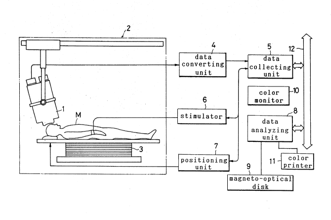
Numeral 2 in Fig. 3 denotes a magnetic shield
room. The magnetic shield room encloses a bed 3 for
supporting an examinee M lying thereon, and a multi-
- 20 -
r , , ., ,,., ;, j ,, . , ,.,, ; , ; . .. .
212~086
channel SQUID sensor 1 disposed adjacent the brain of
the examinee M, for example, for measuring, in a
painless and harmless way, minute magnetic fields
formed by bioelectric current sources occurring in the
brain. ~s noted hereinbefore, the multichannel SQUID
sensor 1 has a multiplicity of magnetic sensors im-
mersed in a coolant within a De~ar. In this embodi-
ment, each magnetic sensor consists of a pair of coils
for detecting a magnetic field component in a radial
direction, with the brain being regarded as a spherical
body.
Field data de,ected by the multichannel SQUID
sensor 1 are applied to a data converting unit 4 for
conversion to digital data to be stored in a data
collecting unit 5. A stimulator 6 applies electric
(acoustic, optical or other) stimulation to the
examinee M. A positioning unit 7 determines a posi-
tional relationship of the examinee to a three-dimen-
sional coordinate system based on the multichannel
SQUID sensor 1. For example, small coils are attached
to a plurality of sites on the examinee M, and the
positioning unit 7 supplies power to these small coils.
Then, the coils generate magnetic fields to be detected
by the multichannel SQUID sensor 1, thereby enabling
25 determination of the position of the examinee M :~
- 21 -
~" ~ " "': , ' ~ . '
F~ . .
.,,:., ,, . . . :
,., . :......... : . . . ~ ,. : . . ; .
~.
`--` 2~25~86
relative to the multichannel SQUID sensor 1. Other
methods may be used to determine tne position of the
examinee M relative to the SQUID sensor 1. For exam-
ple, a projector may be attached to the Dewar to emit a
light beam to the examinee M to determine the position-
al relationship. Various other methods are available
as disclosed in Japanese Patent Publications (Unexam-
ined) No. 5-237Q65 and No. 6-738925.
A data analyzing unit 8 is used to deduce current
sources in a region to be diagnosed of the examinee M,
from the field data stored in the data collecting unit
5. A magneto-optical disk 9 associated with the data
analyzing unit 8 stores sectional images obtained from
a radiographic CT apparatus or MRI apparatus, for
example. The current sources deduced by the data
analyzing unit 8 may be superposed on these sectional
images for display on a color monitor 10 or for print-
ing by a color printer 11. The sectional images
obtained from the radiographic CT apparatus or MRI
apparatus may be transmitted directly to the data
analyzing unit 8 through a communication line 12 shown
n Fig. 3.
A sequence of current source deduction executed by
the data analyzing unit 8 will be described hereinafter
with reference to the flowchart shown in Fig. 4.
- 22 -
~ `~
212~08fi
As noted above, a positional relationship of the
examinee M to the three-dimensional coordinate system
based on the multichannel SQUID sensor 1 is measured
and stored first. Then, as in the prior art illustrat-
ed in Fig. 1, three-dimensional lattice points N are
set evenly in a region to be diagnosed, e.g. the brain,
of the examinee M (step Sl). - -
The respective coefficients in the matrix A
expressed by equation ~3) are computed by Biot-Savart's
law (the coefficients in matrix A being computed each
time the lattice points are moved as described later).
Subsequently, a current source (least norm solution) at
each lattice point is determined by the least norm
method (step S2).
Next, the lattice points are moved toward a
lattice point having a current source of large value
among the current sources determined at step S2 (step
S3). Fig. 5 shows how this step is taken. Reference N
in Fig. 5 denotes the group of lattice points initially
20 set at step Sl. The lattice point marked "x" is the -~
lattice point having a current source of large value
among the current sources determined at step S2. The
other lattice points are moved toward this lattice
point, to form a group of lattice points Nl correspond-
ing in number to the group of lattice points N but
- 23 -
2125086
lying closer together.
Step S3 of moving the other lattice points toward
the lattice point having a current source of large
value may be executed by any suitable method, and the
following is one example. Assume that, by regarding
the size of the current source at each lattice point
determined at step S2 as a mass, and attractive forces
due to gravity act among the lattice points. Then,
each lattice point moves toward a lattice point of
greater mass. The lattice points are collected with
the higher density, the closer they are to a lattice -~
point having a large mass. The moving distance of each - ~-
lattice point is set as appropriate.
Step S4 is executed to check whether a minimum
15 distance between lattice points in the group of lattice ;~
points Nl formed after the movement made at step S4 is
less than a predetermined distance. This distance is
determined as appropriate, based ~sl the precision of
deduced positions of the current sources.
If the minimum distance between lattice points
exceeds the predetermined value, the operation returns
to step S2 to determine, by the least norm method, the
current source of each lattice point in the group of
the lattice points Nl formed by moving the original
lattice points. As noted above, the number of lattice
- 24 -
.
~`~' 212~086
points N1 is the same as the number of original lattice
points N. In the linear equation (5) (set out hereun-
der again) used in the least norm method,
[P'] = A ' [B] ... (5)
the number of elements in vector [P'] is not increased
but is fixed. This means that the computing precision
of the least norm solutions is maintained. On the
other hand, since the lattice points have been moved,
the least norm method executed a second tlme disregards ~ ;;
presence of current sources in hatched regions in Fig.
5. However, these regions are, after all, separate
from a position expected to include a true current
source. The lattice points in these regions have
hardly any chance of including the .rue current source.
lS Thus, there is no fear of lowering the precision of
deduction by excluding these regions.
, . ~ .,
As before, a current source at each of the lattice
points N1 is determined by the least norm method (step ;~;~
S2). It is presumed that a current source of large
value is close to the true current source. Toward the
lattice point having this current source, the other
lattice points are moved to form a new group of lattice
points N2 ~step S3).
When, after repeating the above process, a minimum
distance between lattice points is found to be below
- 25 -
i`-~ 2125086
the predetermined value at step s4, the current sources
of the group of lattice points determined at step S2
executed the last time are regarded as corresponding to
the true current source.
According to this embodiment, as understood from
the foregoing description, the other lattice points are
moved toward the lattice point having a current source
of large value deduced by the least norm method execut-
ed first. Current sources are deduced ~y the least
norm method executed next, with the number of lattice
points remaining unchanged from the previous time, and
with only the distances between the lattice points
diminished. Thus, the current sources may be deduced
with high precision while maintaining the precision in
computing the least norm solutions.
Second Embodiment
Where a plurality of true current sources are
present, the first embodiment poses a question which
lattice point should be selected as one toward which
the other are to be m~ved. The second embodiment
determines likelihood of a current source being present
at each lattice point from deduced physical quantities 1 ~ -
of the current source. Based on the likelihood, the
lattice points are divided into a plurality of groups.
For each group the lattice points are moved toward the
- 26 -
~ 2125086
lattice point having the greatest current source.
The outl~ne of the apparatus and the multichannel
SQUID sensor 1 in this embodiment are the same as in
the first embodiment, and will not be described again.
A sequence of current source deduction will be de-
scribed hereinafter witn reference to the flowchart -~- ~
shown in Fig. 6. - -
As in the first embodiment, three-dimensional
lattice points N are set evenly in a region to be
diagnosed, e.g. the brain, of the examinee M (step
S11).
Then, a current source (least norm solution) at
each lattice point is determined by the least norm -~
method (step S12).
Next, where the position of the "j"th lattice -
point is regarded as vector Vrj, the deduced current
source thereof as vector VPj, the position of the "k"th
(k ~ j) lattice point as vector Vrk, and the deduced
current source thereof as vector VPk, likelihood Q of a
current source being present at the "j"th lattice point
is expressed by the following equation (7), for exam~
ple. This equation is used to determine the likelihood
of presence at each lattice point of the current source
obtained at step S12 (step S13).
':
- 27 -
2125086
Q(Vrj) = ¦VPjj + Y 2 e ~IVrk-Vrjl
k=1, k~j -
In equation (7), ~ is a parameter for adjusting
the degree of likelihood relative to distances between
the lattice paints, and r is a parameter for determin- -
ing a weight of the second term. These parameters are
selected empirically. Further, in the above equation,
"e" is the base of natural logarithm (e = 2.71828 ...),
and "n" is a total number of lattice points.
The first term in equation (7) indicates that the
10 greater the size of the current source at the "j"th -~
lattice point, the greater the likelihood of the
current source being present at this lattice point.
The second term indicates that the higher the density
of lattice points around the "j"th lattice point, the
greater the likelihood of the current source being
present.
In the subsequent processing, lattice points
havin~ less likelihood are moved toward lattice points
of greater likelihood, to deduce current sources from a
more appropriate arrangement of lattice points. To
effect such movement of the lattice points, the lattice
points N are divided into groups by using group func-
tion ~j expressed by the following equation (8), for
example (step S14):
- 28 -
~ 212~086 -
~j(Vrj) = Q(Vrj) e ... (8)
~a :~
Group function ~j indicates influences of the
current source at the "j"th lattice point on the other
lattice points. Vr in e~uation (8) is a position
5 vector of a given point. a is an empirically selected ~
parameter for determining a ~orm of the functions in ~ ~ ;
equation (8).
~A method of dividing the lattice points N into ~- -
groups by using group function ~j will be described
10 with reference to Fig. 7. In the graph shown in Fig. -~
7, the vertical axis represen.s group function ~j, and
the horizontal axis a given position vector Vr.
. .
References A, B and C on the horizontal axis denote ~ ~
-.
lattice points in the group of lattice points N. ~ `-
References ~A, ~B and ~C are group functions ~j of
lattice points A, B and C, respectively. In the
example shown in Fig. 7, the lattice point that gives
the greatest function value at lattice polnt A is B.
In this case, therefore, lattice point A belongs to the
.:. .
same group as lattice point B. On the other hand, the
greatest function value at lattice point C is given by
lattice point C itself. Thus, lattice point C belongs ~
to a different group to lattice points A and B. In ~ ~ -
this way, the lattice points N are divided into a
- 29 -
::
,: . .
: - -::
"'''.",-'.'..
.,. ~:. :
2125~8~
plurality of groups.
The lattice points in each group are moved toward
the lattice point having the greatest function value
~current source size) (step S15). Fig. 8 shows how
5 this step is taken. Reference N in Fig. 8 denotes the ~-
group of lattice points initially set at step S11. The
lattice points marked "x" are the lattice points having
a current source of the greatest value in the respec~
tive groups. The other lattice points in each group -~
10 are moved toward this lattice point, to form a group of ~-
lattice points N1 or N2 lylng closer together. The
number of lattice points in the initial group N equals
the total number of lattice points in the groups of
lattice points N1 and N2. Step S15 of moving the other
lattice points toward the lattice point having the
greatest current source in each group is executed in
the same way as in the first embodiment.
Step S16 is executed to check whether a minimum
distance between lattice points in each group of
lattice points N1 or N2 formed after the movement made
at step S15 is less than a predetermined distance.
This distance is determined as appropriate, based on
the precision of deduced positions of the current
sources.
In the first stage of group division, moving
- 30 -
~ 212S086
distances of the lat~ice points are set so that the
minimum distance between the lattice points exceeds the
predetermined value. Thus, the operation returns to
step S12. The current sources of the rearranged
5 lattice points are determined by the least norm method, - :~
regarding the groups of lattice points N1 and N2 as a -~
new group of lattice points. - -
After the current source of each lattice point in -
the respective groups N1 and N2 is determined, the
likelihood of presence at each lattice point of the
current source is determined for the respective groups
N1 and N2 as before (step S13). Then, the lattice ;-~ -
points in each group N1 or N2 are further divided into~--~--
groups ~step S14). The lattice points in each group
15 are moved (step S15). Fig. 9 shows new groups of ~ ~ -
lattice points N3 to N7 resulting from the above steps. ~ -
When, after repeating the above process, a minimum
distance between lattice points is found to be below
the predetermined value at step S16, the current
sources of the group of lattice points determined at
- step S12 executed the last time are regarded as corre-
sponding to the true current sources.
<simulation>
A simulation was carried out to ascertain validity
25 of the above technique. A ball having an 80mm radius ~--
- 31 -
:`;` 2125086
was conceived as the head acting as the region for
which current sources are deduced. As the magnetic ~ -
sensors S, axial type linear differential gradiometers
(see Fig. lOB) having a 30mm base line were arranged in~ -
5 37 channels over a spherical surface having a 117mm ~-
radius. All the gradiometers had axes extending to the
origin. Current dipoles (current sources) were set in
the ball of the head, and the magnetic fields formed by
the dipoles were calculated by means of Sarvas's
equation (J. Sarvas, Phys. Med. Biol., vol. 32, pp
22, 1987) taking the effect of volume current into
account. These magnetic fields were regarded as
measured magnetic fields. Fig. lOA shows this model.
Next, the space was divided into lattices of 20
cubic millimeters, and 257 lattices lying within the
ball of the head were used as objects of reconstruc-
tion. The sensors S used in this simulation extend in
radial directions "r" of the ball, and therefore cannot
detect magnetic fields formed by current components in
the radial directions. Thus, deduction parameters were
current components in a directions and ~ directions.
The magnetic fields were computed on the assump- ~ ~
tion that two current dipoles acting as cùrrent sources ~ ~-
had the same depth (20,0,50), (-30,0,50). The moment
of both current dipoles were set to ~0,10,0). The
- 32 -
:.,.~, ~,,`.
~ " 212508~
units are mm for the position, and nAm for the moment.
The computed magnetic fields are regarded as measured
values, and the results of deduction carried out in the
above embodiment are shown in Figs. llA and llB. Fig.
llA shows the setting, and Fig. llB shows a reconstruc-
tion. While there are isolated current dipoles, the ~ ~ -
lattices gather around the true values, and the current -
dipoles are reconstructed in the right direction.
Next, a case of setting the two current dipoles to ~-
different depths will be described. The current
dipoles were set to positions (20,0,50~ and (-20,0,30),
and the moment was (0,10,0) for both. The results are
shown in Figs. 12A and 12B. Fig. 12A shows the set-
ting, and Fig. 12B shows a reconstruction. While there ~-
are isolated current dipoles again, the current dipoles
disposed at the different depths can also be recon- ~-
structed substantially correctly.
According to this embodiment, as understood from
the foregoing description, likelihood of current
sources being present on the lattice points is deter-
mined from the physical quantities of the current
sources on the lattice points obtained by the least
.- : -. ..:
norm method. Based on the likelihood, the lattice
points are divided into groups. The other lattice - ~-
points ar~ moved toward the lattice point having the
- 33 -
~. ~- - -
`~ 2~2508~ ~ ~
current source of the greatest function value. The
current sources of the rearranged lattice points are
obtained by the least norm method. Thus, current
sources are deduced by the least norm method, without
increasing the number of lattice points. That is, the
current sources may be deduced with high precision
while maintaining the precision in computing the least -
norm solutions. Even if a plurality of true current
sources are present, each current source may be deduced
with high precision.
Third Embodiment
In what is known as the lattice point moving least
norm method described in the second embodiment, the
parameters, a, ~ and r, must be set empirically. These
parameters are dependent on the positions, sizes and
orientations of the current sources. It is therefore
difficult particularly for an operator having little
experience to set proper values for the parameters
based on isomagnetic field diagrams as described above.
20 The parameters could be set improperly to produce --
results contrary to the true solution.
This embodiment obviates setting of parameters ~
and r, which relate to the likelihood of presence of ~;
the solution on each lattice point, among the above
25 parameters a, 3 and r, to deduce current sources with -
' ' ''' ~", '.'
- 34 ~
212~08~ - `
facility and precision.
Inventors have conducted intensive research and -
found that, by simultaneously measuring the three
orthogonal components (i.e. vector measurement) of the
S magnetic field generated by each in vivo current source
and by using this data in application of the above
lattice point moving least norm method, the current
sources may be deduced properly also by the following
equation (9) in which parameter r in equation (7) is
set to zero ~obviating setting of parameter i~ also)~
Q(Vrj) = ¦VPjl ... (9)
It is believed that the current sources may be -
deduced properly also by equation ~9) not including the
second term of equation ~7) for the following reason.
Generally, as shown in Fig. lOA, the magnetic
sensors S for detecting magnetic fields generated by in
vivo current sources are arranged to have coil axes
thereof extending radially where the area of the
examinee M under examination is a spherical body. As
20 shown in Fig. lOB, each magnetic sensor S has a pair of ~
coils Ll and L2 arranged radially of the spherical body --
~in Z direction in Fig. lOB). Consequently, field data ;~
detected are Z-direction components only. Since only -~
the Z-direction components are detected of the magnetic
25 fields having three orthogonal X-, Y- and Z-direction ` -~
_ 35 -
. ,~"'!
~`- 212~086 ~
components, the field data detected have a low degree
of mutual independence to provide a low spatial resolv-
ing power. Thus, the second term in equation (7), i.e.
the density of current sources adjacent the lattice
points, is considered to have a great influence on
likelihood Q of presence of solutions on the lattice
pointe.
On the other hand, vector measurement of the
magnetic fields generated by in vivo current sources
detects the three orthogonal X-, Y- and Z-direction
components of the magnetic fields in the examinee. The
field data measured have an increased level of mutual
independence to improve the spatial resolving power.
It is thus believed that likelihood Q of presence of
solutions on the lattice points is obtained with high
precision from only the first term in equation (7),
without taking the second term into account.
This embodiment will be described further with
reference to the flowchart shown in Fig. 13.
The multichannel SQUID sensor 1 disposed adjacent
the examinee M is driven to measure simultaneously the
three orthogonal components of minute magnetic fields
in the examinee M (vector measurement) (step S20). The -
magnetic sensors (pickup coils) Sl to Sm of the
multichannel SQUID sensor 1 used here each comprise
.- . .~ ~. ~ ,.. .
- 36 -
~.: - - .. -
` 2125086
three pickup coils having detecting sensitivity in the
three orthogonal directions. This type of pickup coil
may be a three-axis gradiometer, for example. The
gradiometer is formed by dividing the pickup coil into
5 two opposite windings, to cancel uniform magnetic -
fields and detect only magnetic fields having gradi- - ;
ents.
:.
Fig. 14 schematically shows a construction of the
three-axis gradiometer. The pickup coils LX, LY and LZ
detect field components in X, Y and Z directions,
respectively. The three-axis gradiometer is not
; ~ limited to any particular construction. Three-axis
coils may be attached to a cubic core element to be -;-
orthogonal to the six surfaces thereof. A three-axis
15 gradiometer as disclosed in Japanese Patent Publication -~
(Unexam~ned) No. 4-301581 may be used. The latter ~- `
includes a cold temperature resistant flexible material ~ `
rolled into a cylinder, and three pairs of supercon- -~
ducting film coils wound opposite and connected to each
other and formed on surfaces of the flexible material
at varied angles to each other.
Next, three-dimensional lattice points N are set `~
evenly in a region to be diagnosed, e.g. the brain
.. .
(step S21). Then, a current source ~least norm solu-
tion) at each lattice point is determined by the least
-
- 37 - -~
.: ,~ -:
,~,.~
212508~
norm method noted above (step S22).
Next, the likelihood of presence at each lattice
point of the current source is determined using equa-
tion (9) described above (step S23).
To move lattice points havin~ less likelihood
toward lattice points of greater likelihood, the
lattice points N are divided into groups by using group
function ~ expressed by equation (8) (step S24).
Parameter (moving parameterl a in equation (8) is
empirically selected as described hereinbefore.
Next, the lattice points in each group are moved
minute distances toward the lattice point having the
greatest function value (current source size) (step
S25, see Fig. 8). ; ~ -~
The next step S26 is executed to check whether a
minimum distance between lattice points in each group
-. ~
of lattice points (N1 or N2 in Fig. 8) formed after the
movement made at step S25 is less than a predetermined
`distance. This distance is determined as appropriate,
20 based on the precision of deduced positions of the ;~
current sources.
In the first stage of group division, moving
distances of the lattice points are set so that the `~
minimum distance between the lattice points exceeds the
predetermined value. Thus, the operation returns to
- 38 ~
::
-ix 212~086
step S22. The current sources of the rearranged
lattice points are determined by the least norm method,
regarding the groups of lattice points Nl and N2 as a
new group of lattice points. After the current source
of each lattice point in the respective groups Nl and
N2 is determined, the likelihood of presence at each
lattice point of the current source is determined for
the respective groups Nl and N2 as before (step S23).
Then, the lattice points in each group Nl or N2 are -
further divided into groups (step S24). The lattice
points in each group are moved (step S25) to form new
groups of lattice points (N3 to N7 in Fig. 9).
When, after rçpeating the above process, a minimum
distance between lattice points is found to be below
15 the predetermined value at step S26, the current ~ -
sources of the group of lattice points determined at
step S22 executed the last time are regarded as corre~
sponding to the true current sources.
<simulation> ~ -
Simulations were carried out to ascertain validity
of`the above technique. Here, pickup coils as shown in
Fig. 14 were assumed to make vector measurement. The
-~ ~ . ,: ,: :
pickup coils as shown in Fig. lOB were also used to
- . ::: ;.,:
measure only radial components, and magnetic field
- ~ , ,:
generated by the same current source were computed. To
.~ :'~:.':
- 39 ~
:~ ,.
`` 2125086
equalize the conditions for evaluating the two types of
coils, the number of channels and the region for
measurement were set substantially the same. For
vector measurement, the channels were set to 13 X 3 =
39 channels, and the coil pitch to 37.5mm. For radial
measurement, the channels were set to 37 and the coil
pitch to 25mm. The coils were arranged on a ball
having a 117mm radius, with coil axes extending to the
center of the ball. However, since tangential compo-
nents of the magnetic fields are influenced by volumecurrents, the magnetic fields generated by the current
sources were computed using a spherical model to take
the influences of volume currents into account (J. ~ --
Sarvas, Phys. Med. Biol., vol. 32, pp 11-22, 1987). ~ ~-
A deducing simulation was carried out, using -
. .: .. . - . .. ~ ~ . .
equation (9), on each of the field data gained by
vector measurement and radial measurement. A ball
having an~80mm radius was conceived as the head, and
the magnetic sensors were arranged symmetrically about
Z-axis (see Fig. lOA). The sensors were arranged at a
- ~ .
distance of 37mm from the surface of the ball. As the
current sources, two current dipoles were arranged as
follows: ~ ~
position [mm] moment [nAm] ~ -
( 20, 0, 50) (0, 10, 0)
- 40 -
`~-``` 2125D86
(-20, 0, 5) (0, 10, 0)
The results of deduction are shown in Figs. 15A
and 15B. Fig. 15A shows current sources deduced from
the field data of vector measurement. Fig. 15B shows
results of deduction based on the radial measurement.
In the drawings, the circles show set positions of the
current sources, and the arrows show deduced current -
.
sources. As seen from Figs. 15A and lSB, the current
sources are deduced correctly by the technique of this
embodiment which applies the foregoing equation (9) to
the field data obtained from the vector measurement,
: . ~
while the current sources are not deduced correctly
where equation (9) is applied to the field data ob-
tained from the radial measurement.
Thus, this embodiment requires empirical setting
of only parameter a among parameters a, B and r in the
lattice point moving least norm method. The current -
,- ~; .-
sources may be deduced with so much facility and
precision for the non-requirement for setting of
parameters B and Y.
Fourth Embodiment
~ . . .
At step S24 in the third embodiment, parameter
(moving parameter) a is set by experience of the
operator. However, this moving parameter, depending on -~
a value set thereto, could produce a totally different
:
- 41 -
" :~
, - :'~
~` 2125086
result. If this value can be determined by some means~
a deduction technique of high generality requiring no
empirical parameters may be realized in combination
with the technique of the third embodiment described
above.
This embodiment regards the norm of the solution
obtained by the least norm method as a criterion for ~-
determining moving parameter a. With this technique,
the least norm solution is determined by moving the
lattice polnts upon each repetition, and therefore the
norm of the solution changes every time. Thus, varia~
tions in the norm of the solution were checked by
setting various values to moving parameter a for
deduction. Pickup coils for vector measurement as
~lS shown in Fig. 14 were used as sensors. The current
sources and sensors were arranged as in the third
embodiment. Figs. 16A and 16B show norm variations
where a is 0.3 and 0.5, respectively. In Figs. 16A and -~
16B, the horizontal axis represents times of repeti-
20 tion, while the vertical axis represents solution ~ ~ -
norms. Figs. 17A and 17B show results of deduction
thereof. When a is 0.3, the norm of the solution
diverges as shown in Fig. 16A, and produces different ~ ~
deduction results as shown in Fig. 17A. When a is 0.5, ~ --
the norm of the solution converges as shown in Fig.
,' , . ,
- 42 -
~i2~fi
16B, and produces proper deduction results as shown in
Fig. 17B.
These facts show that optimal moving parameter a
may be determined by obtaining lattice point moving
parameter a to minimize the norm of the solution, and
moving the lattice points based on this parameter upon -
each repetition. ~-
A seguence of current source deduction using `-
automatic adjustment of moving parameter a will be
described hereinafter with reference to the flowchart
shown in Fig. 18. -~
Steps S30-S33 in Fig. 18 are the same as steps
S20-S23 of the third embodiment shown in Fig. 13, and
will not be described again.
At step S34, before dividing the lattice points
into groups by using the foregoing equation (8) at step
S35, moving parameter a is optimized by using evalua-
tion function "f" expressed by the following equation
n
J~ -. (10)
In equation (10), VPj(a) is a solution obtained by
the least norm method after moving the lattice points
by using moving parameter a. Thus, evaluation function
"f " is the norm of the solution. ~urther, "n" ~ ~
: ~.
- 43 -
-:
. .
``` 212S086
represents the number of lattice points.
At steps S34 to S36, several parameters al, a2, a3
and so on are applied in advance, the lattice points
are tentatively moved by using these parameters, and
the least norm solutions are obtained, respectively.
These least norm solutions are applied to equation (10) -~
to derive values of evaluation functions f(al), f(a2), : :
; f(a3) and so on. The parameter having the least value
~ is adopted as moving parameter a. The least norm
solution obtained by moving the lattice points based on
the adopted moving parameter a is adopted, and the
least norm solutions based on the other parameters are : ;
discarded.
Then, step S37 is executed to determine an amount -
lS of variation ~f between the norm of the solution
~(evaluation function value fL 1) derived from steps S33
to S36 executed the previous time and the norm of the
solution (evaluation function value fL) derived from
these steps executed this time. If this amount of
variation ~f is below a predetermined value, the
repetition is terminated. Otherwise, the operation
returns to step S33. Steps S33-S36 are repeated until ;
the amount of variation ~f falls below the predeter-
m~ned value.
The technique illustrated in Fig. 18 not only
;" 2125086
requires no empirical parameters a, 3 or Y but employs
the norm of the least norm solution as the condition to
stop the repetition (step S37). Thus, the current
source deduction processing may be stopped after an ~:
5 appropriate number of repetitions. ~ ~-
<simulation>
A simulation was carried out to ascertain validity
.
of the technique of automatically adjusting moving
parameter a. Nineteen pickup coils as shown in Fig. 14
were arranged on a spherical surface to make vector
measurement. Thus, the number of channels was 19 X 3 =
57. The coil pitch was set to 25mm on the spherical
.:,
surface having a 131mm radius. The head was regarded
as a ball having a 80mm radius, and the magnetic fields
were computed taking the effect of volume currents into
account. The sensors were arranged symmetrically about
~- Z-axis, at a distance of 36mm from the ball of the
- : .: ~
head. As the current sources, a plurality of current `~
dipoles were arranged.
The cerebral cortex was assumed to lie inside the
head ball, and three current dipoles were set thereon.
:::
The position and moment of each current dipole are as
follows:
position [mm] moment [nAm]
(-27.08, 4.78, 47.63) (-8.53, 1.50, -5.00)
- 45 -
~ ~ . ~ :. .:
. ~. ~ .
i~
212~086
(-27.08, -4.78, 47.63) (-8.53, -1.50, -5.00)
( 4.91,-56.08, 32.50) ( 0.44, -4.98, -8.66)
Fig. 19 shows the results of current source ~ --
~eduction carried out by the lattice point moving least
norm method while automatically adjusting moving
pa~rameter a. As seen, the current sources are deduced
adjacent proper positions. In deducing the current
sources~by this technigue, a solution is obtained as a
distribution of current dipoles even if the true ~ -
current source comprises a single current dipole. When
the moments of the current dipoles are integrated, the -
value substantially corresponds to the set moment of
the current dipoles, which confirms validity of this
technique.
According to this embodiment, as understood from
the foregoing description, the three orthogonal compo- ~ -
nents of the current sources generated by bioelectric
currents~are detected simultaneously by a plurality of ;;~
magnetic sensors. In the lattice point moving least
. .
norm method, therefore, the likelihood of current
sources being present at the lattice points is deter~
mined by considering the sizes of the current sources
at the lattice points. There is no need for consider-
ing density of the current sources around each latticé
~5 point. It is therefore unnecessary to empirically set
- 46 -
. . :
~bc
~ ,.. , . ,~, . .
~` 212~086 :
parameters for determining levels of influences of the
density of the current sources around each lattice
point on the likelihood of current sources being
present a the lattice points. The current sources may
be deduced with facility and precision accordingly.
Fifth Em~odiment -
The least norm method described above is based on
.
the premise that the number of unknowns 3n (n being the
. .
number of lattice polnts), where the sizes in X, Y and
Z directions of the current sources assumed for the
respective lattice points are taken into account, is
greater than the number of~magnetic sensors m (the
number of equations), i.e. 3n>m. Consequently, coeffi~
cient matrix A in the foregoing equation (2) could be
: - -: ~.
lowered in level (i.e. the same column vector could
appear). This renders the solutions derived unstable.
Further, the least norm method is added only as a
condition for solving simultaneous equation (2). No
clear theoretical basis is provided for minimizing norm
20 I P I of current source [P]. It is therefore difficult .
to conclude whether or not the current sources deduced
by thls method represent a substantially true current
source.
In the lattice point moving least norm methods
proposed in the first and second embodiments also,
- 47 -
~. ~
2125086
whether a minimum distance between lattice points is
below a predetermined convergent criterion is used as a
convergent determination condition for deducing final
current sources in the course of repeating movement of
5 the lattice points and the least norm method. Thus, ~-
deduction results could vary with the predetermined
convergent criterion. This poses a problem of impair- -
ing generality of the deduction method.
This embodiment eliminates the above disadvantag-
10 es. Specifically, this embodiment realizes greater ~ -
accuracy in deducing current sources, requires no
convergent criterion to be set for deduction of current
sources, and enables a final deduction of current
sources to be effected uniformly.
In this embodiment, field data are collected from
the examinee M by the same multichannel SQUID sensor 1
as used in the first and second embodiments. A se-
quence of current source deduction will be described
hereinafter with reference to the flowchart shown in
Fig. 20.
First, three-dimensional lattice points N are set
evenly in a region to be diagnosed, e.g. the brain
(step S41). Here, the number of lattice points N is
selected so that the number of un~nowns 3n is smaller
than the number of magnetic sensors Sl-Sm. This
' ~.
, ' -"
2 1 2 5 0 8 6
enables current sources ~P] to be derived by a linear
least squares method as described later.
Next, step S42 is executed to determine current ~
sources [Pl from magnetic fields [Bd] detected by the ;~ - -
magnetic sensors S1-Sm. The current sources [P] and
magnetic fields [Bd] are in the following relationship
.. .. -
~i ~ as in the foregoing equation (2):
[Bd] = A~P] ~-
As noted hereinbefore, matrix A includes coeffi- -
- .
cient aij representing intensity of a magnetic field
detected in the position of each magnetic sensor S1 to ;;
-~ Sm, where the current sources of unit sizes in X, Y and -~ -~
Z directions are arranged on the lattice points.
Matrix A has 3n X m elements. Thus, current sources ;~
~-- ..
15 [P] can be derived from; - -
[P] = A ~Bd]
as expressed by the foregoing equation (4). However,
- ~ -
no solution is available if the number of equations m
(the number of magnetic sensors S1-Sm) is greater than ~ -
the number of unknowns 3n (the number of current
sources assumed for the lattice points). Then, by
adding a condition to minimize square error ¦~Bd]-[B]~
between measured magnetic fields [Bd~ and current
sources [B] applied to the magnetic sensors S1-Sm by
25 current sources [P] assumed for the respective lattice ~--
:, :
.... : -
~il` 212~086 :
points, current sources [P] may be derived from the
following equation using the well-known linear least
squares method to minimize the square error:
~ P ] = ( AtA ) lAt ~ Bd ] : -
Next, at step S43, the magnetic fields applied to
the magnetic sensors Sl-Sm by current sources [P]
obtained by the linear least squares method at step S42
are derived from the foregoing equation (2), i.e.:
[B] = A[P]
Square error ¦[Bd]-[B]¦ between these magnetic fields
and the magnetic fields actually detected by the
magnetic sensors Sl-Sm are computed, and the square ~ ~
error is checked whether it is a global minimum or not. --
If the square error is a global minimum, it means
that the value is the least among the least square
errors obtained by the above method for the positions
of the respective lattice points when the lattice
~points are moved plural times during repetition of step
S44 described later. Whether the square error is a
global minimum or not may be determined by storing the
least square errors obtained by the method of above - - -
steps S42 and S43 for thè lattice points successively ~ ;
moved in the course of repeating step S44 as described
later, and comparing these square errors to find a
global minimum thereamong. Thus, when the square error
- 50 -
., ,
212~86
, ~ ~;''
obtained is found not to be a minimum at step S43, the
operation proceeds to step S44 to move the lattice
points. If the square error is found to be a minimum,
the operation proceeds to step S45 to finally deduce
current sources [Pl.
At step S44, the lattice points are divided into a ~
plurality of groups and moved based on the likelihood - `
of a current source being present at each lattice
point. Computation of the likelihood of a current ~ ~ -
source being present at each lattice point, and divi-
sion into groups and movement of the lattice points ~
based thereon, are carried out using eguations (7) and -
(8) as in the second embodiment, and will not be ~ -
described again.
After moving the lattice points, the operation ;
returns to step S42 to obtain current sources [P} for
the moved lattice points. This and previous computa- `~
tions are different in coefficients of matrix A identi-
. ~
fied by the position of each lattice point. Step S43 -~
20 is executed again to determine whether the square error -~
is a minimum or not. If the square error is found not
to be a minimum, steps S42-S44 are repeated. If the
square error is found to be a minimum, step S45 is
executed to regard current sources [P] providing the
minimum current source [B] as the true current source.
- 51 -
~! 212 5 0 8 6
This completes the processing sequence.
<simulation>
A simulation was carried out to ascertain func-
tions of the above technique visually. Figs. 21
through 23 show a three-dimensional arrangement of
lattice points, assuming that the number of lattice
poir.ts n is 28, and the number of magnetic sensors m is
129. It is further assumed that a current source (5.6,
5.6, -6.0) [nAm] is present in the position marked with
a circle (16.0, 16.0, 30.0) [mm]. The arrows and black
spots lndicate the lattice points. Lattice points
having large current values are indicated by large
black spots. Lattice points having larger current
values are indicated by the arrows. Lattice points
having small current vaIues do not appear in these
drawings. Thus, the drawings show fewer lattice points -
than the actual number thereof.~
Fig. 21 shows current sources [P] deduced immedi-
:
ately after the lattice points were set evenly. The
square error was f=1.454925e~3 at this time. Fig. 22
shows current sources [P] after the lattice points were
moved plural times. It will be seen that, compared ;;~ ~
with Fig. 21, the lattice points have been collected ~ ;
around the true current source. The lattice points -
having large current values as indicated by the arrows
- 52 -
~ ` 212508~
appear adjacent the true current source. The square
error was f=4.119901e 06 at this time. Fig. 23 shows
positions of the current sources when the square error
is minimized. The plurality of lattice points having ~-
large current values as indicated by the arrows in Fig.
22 now overlap the true current source, showing that
the true current source is deduced correctly.
As described above, this embodiment employs the
magnetic sensors larger in number than the unknowns
corresponding to the set lattice points. Thus, stable
solutions ~current sources ~P]) are derived from the
magnetic fields [Bd] measured by the magnetic sensors.
The current sources are derived from the measured
magnetic fields on condition that the square error ~ -
between the magnetic fields [B] due to unknown current
sources [P] at the lattice points and the magnetic
fields [Bd] measured by the magnetic sensors is mini-
mized. This allows the current sources [P] to be `~
deduced accurately. In addition, the current sources
~P] occurring when this square error is a global
minimum is regarded as the true current source. It is -~
therefore unnecessary to set a convergent criterion for
deducing final current sources, thereby allowing a
uniform deduction of final current sources. -~
- 53 -
, . . .
2125086
Sixth Embodiment
The fifth embodiment described above uses group
functions, and therefore requires parameters to be set
for deduction of current sources. Further, since the
lattice points are moved little by little within each
group, the lattice points are moved a large number of
times and a considerable time is consumed in computa-
; tion before results of deduction are produced. This
embodiment overcomes these disadvantages of the fifth
embodiment. This embodiment requires no parametersetting, and moves the lattice points at a time, to
allow current sources to be deduced in a short time.
This embodiment will be described hereinafter with
reference to the flowchart shown in Fig. 24.
First, at step S51, lattice points are set evenly
:
in a region to be diagnosed, as in the fifth embodi-
ment. Then, step S52 is executed to determine unknown
current sources [P] at the respective lattice points by
the least norm method. At step S53, the square error
- ~20 between magnetic fields lB] derived from the current
sources [P] obtained at step S52 and magnetic fields -
[Bd] actually detected by the magnetic sensors S1-Sm is
.~, ~. .:
checked whether it is a global minimum or not. ~ ~ -
If the square error is found not to be a global
25 minimum at step S53, the operation proceeds to step S54 - - ;
. : ..
54
'' .' `~`~`'~'`
...:.. .~ .
~`"` 212508fi
for newly determining current sources at the lattice
points under the condition to minimize evaluation
function f to which a penalty term is added as follows:
n 2 3m
f = ~ (Bdi-Bi) + ~ ~ (wi Pi2) ... (11)
i=l i=l
In this case, A in equation (5), [P] = A [B],
can be derived from the following equation (12):
A = (A A+~-W) 1-At ... (12)
where
wl '~
w2 0
W = w3 -- (13)
O . :. ;.
w3n -~
15Generally, the closer current source Pi is to a
field measuring plane, the greater current source is -~
measured. Thus, by setting matrix W as follows, for
example;
m ~-~
Wi = ~ Aji2 ---(14)
j=l .. ~
the influence of the distance to the field measuring
plane may be canceled for current source Pi derived.
Further, the term of the square error of magnetic
fields (AtA) and the penalty term (W) may be substan-
tially equalized by setting weight A f the penalty
term to ¦AtAI/lW~
~ .
: ~ . .
- 55 -
.., .,., ~...
2125086
Thus, current sources P on the respective lattice
points are derived from equations ~5) and (12). At
step S55, the lattice points are moved to the vicinity
of the lattice point having the greatest of the current
sources P determined at step S54. In the mode of
movement employed here, without being limitative, eight
lattice points having small currents deduced are moved
to the corners of a cube with the lattice point of the
greatest current deduced lying in the center thereof.
10 The cube has a size corresponding to a half of the -~
distance between the lattice point of the greatest
current deduced and the lattice point closest thereto. -
After moving the lattice points in the above -~
sequence, the operation returns to step S52 for newly
~ 15 obtaining current sources [P} for the moved lattice
;~points. Then, step SS3 is executed again to determine ;~
~; whether the square error is a global minimum or not.
If the square error is found not to be a minimum, steps
. . ,
S52-S55 are repeated. If the square error is found to
be a global minimum at step S53, step S56 is executed
to regard current source [P] providing the globally ~ -
minimum current source [B] as the true current source. ^` ` -
This completes the processing sequence.
According to this embodiment, current sources are
determined invariably by using the evaluation function
' ,,,; :..' ,-
- 56 -
' ' ':
" ;~
2125086
in moving the current sources at the lattice points.
The greatest current source may be determined by a
simplified sequence. Further, since the penalty term
which is a weighted sum of squares of the current
sources is added to the evaluation function, stable
solutions are obtained even where the lattice points
are not in the true current source. This allows the
lattice points to be moved at a time to the vicinity of
the greatest current source. The greatest current
source may be determined without using the group
function described in the fifth embodiment. Conse~
quently, this embodiment dispenses with a complicated
seguence, for example, of setting parameters for -
deducing the current sources. In the fifth embodiment,
the lattice points are moved little by little within
each group. Consequently, the lattice points are moved
a large number of times and a considerable time is
:. ~ .. -
consumed in computation before results are produced.
In the sixth embodiment, as described above, the
.. ..
20 ~ lattice points are moved at a time, thereby allowing -~
the current sources to be deduced in a short time.
<simulation>
Simulations were carried out to ascertain func- ;
tions of the above technique visually. Fig. 25 shows
results of a simulation of the fifth embodiment for
- 57 - ;
~-``` 2125086
which improper parameter setting is assumed. Fig. 26
shows results of current source deduction done with the
penalty term removed from the evaluation function in
equation (11) noted above. Figs. 27 through 29 are
results of the simulation showing the current sources
deduced in the sixth embodiment. Each of Figs. 25
through 29 shows a three-dimensional arrangement of
lattice points, assuming that the number of lattice
points n is 32 and the number of magnetic sensors m is ~ ~;
129, and that a current source (-10~2, 10¦2, 0) [nAm] -~
- is present in the position marked with a circle (16.0,
16.0, 60.0) [mm]. The arrows and black spots indicate ~ ~ -
the lattice points. Lattice points having large
current values are indicated by large black spots.
Latti¢e polnts having larger current values are indi-
cated by the arrows. Lattice points having small
c~urrent~values do not appear in these drawings. Thus,
~- f the drawings show fewer lattice points than the actual
number thereof, i.e. 3~2. ; -~-
As shown in Fig. 25, the true current source is ` `~
not deduced correctly if wrong parameter setting is -~
. . . -. -
made in the fifth embodiment. According to the sixth
em~odiment, as shown in Figs. 27 through 29, as the
lattice points are moved repeatedly, a plurality of
current sources seen in Fig. 27 approach the true
;
- 58 - '
- "~ ' '.
2125086
current source, and ultimately overlap the true current
source as shown in Fig. 29, thereby allowing the true
current source to be deduced correctly.
Seventh Embodiment
The fifth and sixth embodiments described above
determine current sources at the respective lattice
points by the linear least squares method. If noise
mixes into the magnetic fields measured, noise compo-
nents may also be calculated as solutions (current
sources). This results in the disadvantage that the
position of each current source deduced tends to vary.
This embodiment is intended to eliminate the instabili~
-ty due to such noise components.
This embodiment will be described hereinafter with
- -:.
reference to the flowchart shown in Fig. 30.
At step S61, three-dimensional lattice points N
are set evenly in a region to be diagnosed, e.g. the
brain, as in the fifth and sixth embodiments. Here
again, the number of lattice points N is selected so
20 that the number of unknowns 3n lS smaller than the - -~
number of magnetic sensors S1-Sm.
Next, step S62 is executed to determine current
sources [P] from magnetic fields [Bd] detected by the
magnetic sensors S1-Sm, using e~uation (4) noted
hereinbefore.
- 59 -
~;~ 212S086
~P] = A [Bd] ... (4)
Matrix A includes 3n X m elements as expressed by
equation (3) also noted hereinbefore.
With equation (4), no solution is available since
5 the number of equations m (the number of magnetic ~ -~
sensors S1-Sm) is greater than the number of unknowns
3n (the number of current sources assumed for the
lattice points). Thus, current sources [P] are derived
using the linear least squares method by adding a -
condition to minimize evaluation function f expressed
by a sum of square error ¦[Bd]-~B]¦ between measured
magnetic fields ~Bd] and current sources ~B] applied to
the magnetic sensors S1-Sm by current sources [P]
assumed for the respective lattice points, and the
15 penalty term shown hereunder. This evaluation function ;~
is the same as~equation (11) described in the sixth
- embodimènt, which is set out below again.
n 3m
f = E: (Bdi-~i)2 +A ~ (wi-Pi2) ... (11)
By adding the condition to minimize evaluation
function f, equation (4) is rewritten as~
~P] = A ~B] ... (5)
A+ can be derived from equation ~12) described in the ;
sixth embodiment.
The second, penalty term in equation (llJ has the
- 60 -
-
~':,
212S086
smaller value, the closer the current sources lie to
one another. Consequently, noise components occurring ~ -
discretely have no chance of being adopted as solu-
tions.
After current sources lP] are determined, step S63 ~ -
is executed to check whether the sum of square error
between current sources [B] applied to the magnetic
sensors Sl-Sm by current sources [P] assumed and
measured magnetic fields [Bd], and the above penalty
term, is a global minimum or not. If the sum is found
not to be a global minimum, the operation proceeds to
step S64 for moving the lattice points to the vicinity
of the lattice point having the greatest of current
sources ~P] obtained at step~S62.
After moving the lattice points, the operation
returns to step S62 for newly obtaining current sources
;[P] for the moved lattice points by the linear least
squares method, adding the condition to minimize the
eva1uation function as noted above. Then, step S63 is
20 executed again to determine whether the sum of the - -
square error and penalty term is a global minimum or
not. If the sum is found not to be a minimum, steps
S62-S64 are repeated. If the sum is found to be a
g~obal minimum at step S63, step S65 is executed to
regard current source ~P] providing the globally
- 61 -
`~
212~086
minimum current source [B] as the true current source.
This completes the processing sequence.
<simulation>
Simulations were carried out to ascertain func-
tions of the above technique visually. Fig. 31 shows
~; 5 results of a simulation of the foregoing sixth embodi-
ment which assumes that a current sources (-10/~2,
10/J2, 0) ~nAm] is present in the position (16.0, 16.0,
48.0) [mm], and 32 lattice points are set to magnetic ---
fields determined by measuring these current sources
10 with 129 magnetic sensors (with a signal to noise ratio ~ ;
= 20). According to the sixth embodiment, the current
sources obtained are scattered under the influence of
noise.
Fig. 32 shows results of a simulation of the
seventh embodiment which assumes that a current source
(10, 0, 0) ~nAm] is present in the position ~0, 10,
69.0) ~mm~, a current source ~10, 0, 0) [nAm] in the
position (0, -10, 49.0) ~mm], and 32 lattice points are
set to magnetic fields determined by measuring these
magnetic fields with 129 magnetic sensors (with a
signal to noise ratio = 20). It is seen that, accord-
ing to this embodiment, the current sources are deduced
accurately even if noise is mixed into the magnetic
fields measured.
- 62 -
212508~
Eiqhth Embodiment
The technique described in the seventh embodiment
is capable of excellent deduction where the current
sources are assumed to be current dipoles. However,
the current sources deduced tend to consolidate (or
concentrate locally) since the penalty term is added to
the particular criterion for an optimal current source
~step S63 in Fig. 30). This results in the disadvan~
tage that, where current sources are distributed over a
certain range, such current sources are difficult to
deduce correctly. In vlew of this disadvantage, this
embodiment is intended to correctly déduce distributed
current sources.
This embodiment will be described hereinafter with
reference to the flowchart shown in Fig. 33.
; At step S71, lattice points are set evenly in a
region to be diagnosed, as in the seventh embodiment.
Then, step S72 is executed to determine current sources
~P] from magnetic fields [Bd] detected by the magnetic
sensors S1-Sm, using the linear least squares method.
At this time, as at step S62 in the seventh embodiment,
this embodiment also adds the condition to minimize
evaluation function f expressed by the sum of square
error ¦[Bd]-[B]¦ between measured magnetic fields CBd]
and current sources [B] applied to the magnetic sensors
- 63 -
- ' - ~ -
,X,~, ,"~,,",",;.~
,`'.' .~.. ~, '
` 2125086
S1-Sm by current sources [P] assumed for the respective
lattice points, and the penalty term.
Here, weight ~ of the penalty term in equation
(11) is determined according to distances between
lattice points. Specifically, a distance between each
lattice point and the lattice point closest thereto is
determined. Then, weight ~ is determined using an
average of the distances such that the smaller the
average is, the smaller wei~ht ~is. Consequently, -~ -
weight ~ increases when the lattice points are scat~
tered, thereby increasing the influence of the penalty
term in equation ~11). In this way, variations in the
deduced current sources due to noise components may be
suppressed. On the other hand, weight ~ decreases when
the lattice points are locally concentrated, thereby
; diminishing the influence of the penalty term in
equation (11). Thus, an undue concentration of the
current sources may be avoided. ~-
After current sources [P] are determined, step S73 ~ ;
is executed to check whether the square error between
current sources [B] applied to the magnetic sensors --
S1-Sm by current sources [P] assumed and measured
magnetic fields [Bd] is a global minimum or not. That
is, since the penalty term is excluded from the partic- -
ular criterion for optimal current sources, adoption of
'' ~..~.:
- 64 -
"`' '.-~ `';.` ".
~ "~} ~ "~ " ~"~
212508fi
unnecessarily concentrated current souxces as optimal
current sources is avoided. If the square error is
found not to be a global minimum, the operation pro-
ceeds to step S74 for moving the lattice points to the
vicinity of the lattice point having the greatest
current source as in the seventh embodiment. Then, the
operation returns to step S72 for newly obtaining -~
current sources ~P] for the moved lattice points by the
linear least squares method to which the penalty term
0 lS added as before. Then, step S73 is executed again -~
to determine whether the square error is a global
minimum or not. If the square error is found not to be
a minimum, steps S72-S74 are repeated. If the square
error is found to be a global minimum at step S67, step ~ -
575 is executed to regard current source [P] providing
the globally minimum current source [B] as the true
current source. This completes the processing se-
quence.
<simulation>
Simulations were carried out to ascertain func-
tions of the above technique visually. Fig. 34 shows
results of a simulation of the foregoing seventh
embodiment which assumes that current sources of lOnA
are uniformly distributed around a position (0, 20, 60)
[mm] in a cube of 20mm at each side. Based on the
: ': '
- 65 -
.
' ~' : .
~`~
212508~
magnetic fields determined by measuring these magnetic
fields in a uniform distribution with 129 magnetic
sensors (with a signal to noise ratio = 20), 32 lattice
points are set. According to the technique of the
seventh embodiment, the current sources deduced are
excessively concentrated. Fig. 35 shows results of a ~ ;
simulation of the eighth embodiment in which a similar
uniform distribution of current sources are deduced.
It is seen that, according to the eighth embodiment, -
10 the current sources in the uniform distribution are ~
deduced in a correct form. ~ -
The present invention may be embodied in other -
specific forms without departing from the spirit or
essential attributes thereof and, accordingly, refer-
ence should be made to the appended claims, rather than
to the foregoing specification, as indicating the scope
of the invention.
- 66 -