Note: Descriptions are shown in the official language in which they were submitted.
CA 02228~94 1998-02-0~
WO 97/05969 PCT/CA96/00516
M~THOD OF SORTING PI~ OF ~AT~RI~T
TF~cHNIc~Tl FI~T.n
This invention relates to the field of sorting pieces
of material into output batches having predetermined
composition targets.
R ~CKGROUN~ A~T
Sorting pieces of material composed of aluminum (Al),
non-Al metallic compositions (such as stainless steel,
brass, bronze, and zinc alloys) and polymers into
output batches having a predetermined composition
established to maximize the value of the output is
becoming an increasingly important function in the
blending and reprocessing industry.
Prior art material processing systems are generally
directed to either optimized bulk blending or real-
time piece-by-piece sorting with no blending.
For example, a blending system developed by Keystone
Systems, Inc. called the Alloy Blending System (ABS)
involves the optimized blending of melting furnace
composition from bulk material having known aggregate
compositions. The ABS uses off-line optimization to
generate the best groupings of material into output
batches to m~; m; ze the aggregate value of the
outputs. In particular, ABS determines, in advance of
the physical sorting function, the optimal grouping of
material into output batches to maximize the value of
the input material.
The optimization is a relatively slow procedure due to
the extensive processing required to calculate the
optimum output batches. It is suitable for bulk
blending applications such as melting furnace batching
CA 02228~94 l998-02-0~
W097/05969 PCT/CA96/00516
but it is too slow ~or making real-time piece-by-piece
sorting decisions.
A system where optimization is used to re~ine sorting
parameters without blending is disclosed in United
States Patent No. 5,333,739 (Stelte) issued on August
2, 1994. Stelte teaches a method ~or sorting bulk
material, such as scrap glass. Stelte focuses on the
logic required to m;n;m;ze the cross contamination o~
the groups of items being sorted due to the
variability in the item properties and in the
imprecision o~ the analytical method. The objective
of Stelte is to sort the material by the pre-existing
groups in the bulk input material and to minimize the
cross contamination in the sorted groups.
To increase sorting speed, real-time sequential
sorting systems have been proposed in the prior art.
For example, United States Patent No. 5,042,947 issued
August 27, 1995 entitled Scrap Detector discloses a
process ~or analysing metal particles to determine
their composition and to generate a sorting signal.
However, real-time sorting systems do not approximate
an of~-line optimised blending solution (~rom the ABS,
for example), since only the composition o~ the
currently analysed piece is considered in making the
real-time sorting decision.
In summary, sorting and blending systems of the prior
art principally involve two methods. The first is an
optimized batching procedure involving pre-processing
to assign output bin designations to each piece o~
material having known compositions prior to the actual
physical sorting process. The second is a real-time
sorting process that does not require pre-processing,
but does not accurately approximate an optimized
solution.
CA 02228~94 1998-02-0~
W097/05969 PCT/CA96/00516
Consequently, there is a need for a method of sorting
pieces of material that combines the advantages of
optimized batching with the speed of real-time
sequential sorting.
In particular, there is a need for a method of sorting
pieces of material in which sorting parameters are
established to permit real-time piece-by-piece
batching that approximates global optimized results
of blending pieces having different compositions to
arrive at the compositions of the sorted products that
are required by the customers. These output product
compositions are, in general, different than the
composition of any group pre-existing in the unsorted
starting material.
DIS~TOSURT~'. OF T~ INV~TION
An object of the present invention is to provide a
method of sequentially sorting pieces of material
that accurately approximates an optimized solution,
that is one which optimally mixes different
compositions to arrive at pre-determined compositions
of sorted product.
Another object of the present invention is to provide
a method of sequentially sorting pieces of material
that optimally mixes pieces having different
compositions to arrive at predetermined compositions
of sorted product.
Another object of the present invention is to provide
a method of piece-by-piece batching that minimizes the
number of output groups and minimizes the amount of
input material that has to be downgraded into low
value compositions.
CA 02228~94 1998-02-0~
W097/05969 PCT/CA96/00516
In accordance with one aspect of the invention there
is provided a method of sequentially sorting an input
batch of pieces of material each having a composition
defined by at least one control element, each of said
pieces having a concentration for each of the control
elements and a weight, said sorting being from the
input batch into a plurality of output bins each
assigned a target concentration for each of the
control elements, pieces in each of said output bins
having a cumulative aggregate weight and an aggregate
concentration for each of the control elements,
comprising the steps of: (a) establishing a bin order
for a selected one of said pieces; (b) calculating in
the bin order an aggregate composition of the output
bins after the addition of said selected piece; (c)
placing the selected piece in a selected bin, said
selected bin being the first bin for which the new
aggregate composition falls within the target
concentration limits for all the control elements; and
(d) repeating steps (a) to (c) for each subsequent
piece in the input batch.
In accordance with another aspect of the present
invention there is provided a method of sequentially
sorting an input batch of pieces of material each
having a composition defined by at least one control
element, each of said pieces having a concentration
for each of the control elements and a weight, said
sorting being from the input batch into a plurality of
output bins based on a plurality of predetermined
sequential sort parameters, comprising the steps of:
(a) establishing a bin order for a current one of said
pieces; (b) calculating in the bin order an aggregate
composition of the output bins after the addition of
said current piece; (c) placing the current piece in a
bin for which the new aggregate composition falls
within limits established by the sequential sort
CA 02228~94 1998-02-0~
W O 97/05969 PCT/C A96/00516
parameters; and (d) repeating steps (a) to (c) for all
subsequent pieces.
RRIEF DFSCRIPTION OF T~ DRAWINGS
Embodiments of the invention will be described by way
of example in conjunction with the drawings in which:
Fig. 1 illustrates a schematic representation of
a sequential material sorting apparatus;
Fig. 2 represents a flow chart of a piece
specific bin ordering method according to an
embodiment of the present invention;
Fig. 3 represents a flow chart of a piece
specific bin ordering method according to another
embodiment of the present invention; and
Fig. 4 represents a flow chart of fixed bin
ordering methods according to an embodiment of the
present invention.
R~T MODE(S) FOR C~RRYING OUT T~F INV~NTION
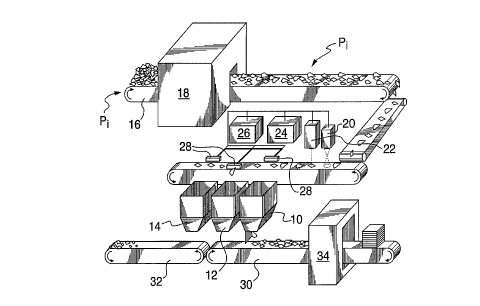
Referring to Fig. 1, numerals 10, 12, and 14 represent
three output bins used to hold pieces of material of
various compositions designated generally as Pi. The
pieces Pi are loaded on a conveyor belt 16 that feeds
the pieces Pi into a material preparation area 18
where the pieces are distributed on the conveyor 16.
Each piece Pi passes under a trigger device 20 to
signal a laser 22 that another piece Pi is to be
analyzed.
A spectrometer 24 reads the reflections of the laser
22 and supplies the data to a computer 26. The
computer 26 processes this information to direct the
diverter arms 28 to place the pieces Pi into one of
the output bins (10, 12 or 14). The output bins can
then deposit their contents onto output conveyors 30
and 32 with conveyor 30 leading to a bailing station
CA 02228~94 l998-02-0~
WO97/05969 PCT/CA96/00516
34 and conveyor 32 leading to a ~oundry processing
station (not shown).
The three output bins are illustrative only, and the
actual number of output bins is dependent on the
particular input batch of material being sorted and
customer driven output requirements. The real-time
piece-by-piece sorting methods of the present
invention will be discussed in conjunction with
aluminum alloy scrap. However, the methods described
can readily be adapted ~or sorting non-aluminum
compositions (such as Mg and Zn alloys, stainless
steel, brass, bronze) and polymers.
Further, the methods described also apply in sorting
any mixture comprised of individual pieces of
material. For example, in the case of a manufacturing
process that by its nature produces at some stage a
mixture of different pieces that requires a sorting
step to batch the input pieces in a plurality of pre-
specified output groups.
The output bins 10-14 are assigned target compositions
and weight levels based on customer requirements or
based on information obtained from historical sorting
runs for similar input material. For example, in the
case of sorting alllm;nl~m, the bins 10, 12, and 14 will
each have prescribed maximum levels of the six major
alloying elements (Cu, Fe, Mg, Mn, Si and Mn) and a
prescribed maximum (target) bin weight.
Input batches are considered similar when their
associated unique composition table contains like
compositions in a like weight distribution. A unique
composition table summarises data on the composition
of an input batch containing hundreds of thousands of
individual pieces. It is a weight distribution table
CA 02228~94 1998-02-0~
W097/05969 PCT/CA96/00516
of unlque combinations of control elements. It is the
basic starting point ~or all off-line calculations
including histogram generation and global
optimization, which will be discussed in further
detail hereinbelow.
Each piece Pi is analyzed sequentially in real-time to
determine the following information:
(a) piece composition; and
(b) piece weight (actual or estimated).
To determine the actual composition of each piece Pi a
composition analysis method is used such as laser
induced breakdown spectroscopy (LIBS) or X-RAY
Fluorescence (XRF). For example, LIBS supplies
information of the chemical composition of the six
alloying elements, and on selected trace elements that
may be found in large concentrations in some aluminum
alloy (i.e. Li, Sn, Cr and Ni).
During real-time sorting of pieces of material it is
not normally possible to weigh each individual piece
Pi to obtain an actual piece weight due to the high
sorting speed. However, an estimate of the piece
weight is necessary for the sorting calculations.
Consequently, after a historical optimized sort of a
similar input batch the weight of the material in each
output bin lO, 12, or 14 and the number of pieces Pi
sorted in each bin is known. A calculated average
piece weight can provide an estimate of the actual
piece weight, which is used to drive the real-time
sequential sorting process.
The inventors have found that for most practical cases
of randomly shredded piece of material where piece
composition is not correlated with piece weight,
calculated average piece weight for the entire batch
CA 02228~94 1998-02-0~
W O 97/05969 PCT/CA96/00516
of material i8 sufficient because random error
averages out over the large number o~ pieces sorted
Specifically, sorting based on estimated piece weight,
or fixed weight (for all pieces being sorted) instead
of actual piece weight was ~ound to yield very similar
sorting results. Further, it was also found that the
sorting results were insensitive to the fixed weight
assigned to each piece.
For example, sorting with both 50g and 200g fixed
piece weights produced the same composition error in
trial experiments, equal to approximately 8~. This is
a reasonable result since scaling piece weights from
50g to 200g does not a~fect how pure pieces balance
impure pieces. Balancing a 200g impure piece with a
200g pure piece is exactly the same as balancing with
50g pieces.
After the actual composition and estimated weight of
each piece Pi have been obtained, it is assigned a bin
order. The bin order is used during a composition
check in which each piece Pi is compared to the output
bin target composition.
Each piece Pi is placed into the first bin that can
accept the piece without exceeding the m~; ml7m control
element concentrations prescribed by the output bin.
The term "element" in the context of "control element
referenced in the present application refers to a
constituent that is a part of a complex whole. For
example, control elements can represent an actual
Periodic Table element, molecular constituents,
material subcomponents and the like.
CA 02228~94 1998-02-0~
W O 97/05969 PCT/CA96/00516
The bin order for each piece Pi is established using
one of the following methods:
(A) Fixed bin order giving priority to the output
bin with the highest output weight target.
For example, if bins 10, 12, and 14 were
assigned absolute target weights of x, y,
and z (units) respectively, where x>y~z,
then the bin order for each piece Pi would
be [bin 10; bin 12; bin 14].
(B) Modified fixed bin order in which priority is
given to the high value output bin with the
highest target concentration of alloying
elements.
For example, assume the same weight
information recited in (1), if bin 12 has
the highest target concentration of alloying
elements (relative to bins 10 and 14), then
the bin order for each piece Pi would be
[bin 12; bin 10; bin 14]. Bin 12 takes
priority ranking order over the heavier
target weight of bin 10 due to the target
composition of the bin.
(C) Piece specific bin order that gives higher
priority to the output bin having the best match
with the composition of the current piece.
For example, if the bins were assigned the
following composition targets:
(a) bin 10 Cu=a, Fe=b, Mg=c, Mn=d,
Si=d, Zn=d;
(b) bin 12 Cu=b, Fe=a, Mg=f, Mn=a,
Si=a, Zn=a; and
CA 02228~94 l998-02-0~
W097/05969 PCT/CA96/005l6
(c) bin 14 Cu=a, Fe=d, Mg=e, Mn=a,
Si=e, Zn=a,
where a-f designate control
element concentrations expressed
in terms of a batch weight
histogram to be described
hereinbelow; and
a current piece being sorted,
designated P1 has a composition of
Cu=a; Fe=d, Mg=c, Mn=a, Si=e, Zn=c then
the piece order for P1 would be [bin
14; bin lO; bin 12]. Bin 14 is listed
first because the piece P1 is the best
composition match (4 of 6 elements) in
comparison to bin lO (2 of 6 elements)
and bin 12 (1 of 6 elements). Bin lO is
listed second because the piece P1 is a
better composition match in comparison
to
bin 12.
(D) Piece specific bin order that is determined
by a closest match with the destination
distribution of a batch of similar input material
when sorted according to an optimized method.
For example, assume the target compositions
of the bins (10-14) as outlined above, using
historical data more of the material with
the composition of the current piece P1
would have been placed in bin 12 than bin
lO, or bin 14. Consequently, the bin order
for piece P1 would be [bin 12; bin lO; bin
14].
35 To provide data to the sorting methods described
above, a procedure termed by the inventors' as a
global optimization calculation is used to define the
CA 02228~94 l998-02-0~
W097/05969 PCT/CA96/00516
11 '
sort parameters for the real-time sequential sort.
Using standard linear programming techniques various
parameters can be defined including target bin
compositions, target prime dilution/hardener levels,
target optimum quantities for each output bin, and
distribution of the material compositions to the
output bins. The sort parameters of the global
optimization procedure are used to guide the actual
real time sorting methods of the present invention.
Specifically, global optimization involves a solution
of a model consisting of a system of algebraic
equations and non-equality constraints that permits
optimization of blending of individual pieces into
output bins with pre-determined composition. This
model is designed to maximize total dollar value of
alloys produced while maintaining customer specified
composition limits in the output bins.
The material in each output bin is assigned a value in
dollars per unit weight (e.g. $/lb; $/kg etc.) before
optimization begins. The net dollar value of sorted
material in each bin after sorting equals bin weight
multiplied by bin alloy value minus cost of additional
input materials such as sorted scrap, alloying
hardeners and pure prime material.
In addition to the maximum net dollar value for sorted
material collected in all output bins, the optimum
model solution can specify distribution of each unique
composition among output bins, the target bin
compositions and weights for the sorted pieces of
material.
A customer generally specifies the required output
weight, the output composition after dilution and
addition of hardeners and the current market price for
CA 02228594 1998-02-0~
W O 97/05969 PCT/CA96/00516
12
each output composition. These factors are used as
constraints on the global optimization calculation
performed on a historical input batch of material
characterized by similar weight distribution among the
unique compositions. These calculations yield sorting
parameters (A to C): target bin composition limits
(parameter B), final bin weights (parameter C), and
the distribution histogram of the material weight for
each output bin (parameter A).
If the global optimization calculation is not done
parameters B and C can be arbitrarily set and
parameter A can be replaced by a histogram of
distribution of input material weight among the
control element concentration intervals (parameter D).
In this case, however, there is generally no assurance
that the output targets can actually be met during
actual sorting.
In summary, a subset of the following sort parameters
generated from the global optimization calculation are
provided to the real-time sequential sorting methods
of the present invention as discussed in detail
hereinbelow:
p~r~meter A rOutput B; n ~; s~ogram (wt~)l:
Percent of input material element weight
found at each concentration interval for all
control elements, one histogram being used
per output bin;
Par;~meter R rCom~os;t; on T;m;t (m~c;mum
wt~)l: Composition limits, six control
elements are set per bin;
CA 02228~94 l998-02-o~
W097/05969 PCT/CA96/00516
13
Par~meter C rF; n~l B; n Weiqh~ (wt~ Bin
weight as weight percent of input material,
one final weight being set per bin; and
p~r~meter D rR~tch We;ght Histogram (wt~)l:
Percent of input material weight found at
each concentration interval for all control
elements, one histogram being defined per
input batch.
Piece Specific Bin Order Using Batch Weight Histogram
Referring to Fig. 2, a sequential sorting method 95
according to an embodiment of the present invention is
illustrated in the form of a flow chart.
Setup section 98 is performed in steps 100-and 102 to
prepare for the sequential real-time sorting of pieces
of material. Sorting method 95 uses parameter D
(batch weight histogram) from historical batch
composition data, and parameters B (bin composition
limits) and C (final bin weight).
Step 102 specifies the maximum allowable bin
composition limits for all control elements for the
output bins before adding diluents. For example, the
target compositions for bins 10, 12 and 14 could be
defined as:
(a) bin 10: [A] having the following
concentration limits (in relative percentages):
0.4~ Fe; 1.0~ Mn; 0.3~ Mg; 0.2~ Si; 0.04~ Zn; and
0.15~ Cu;
(b) bin 12: [B] having the following
concentration limits: 0.26~ Fe; 0.3~ Mn; 1.6~ Mg;
0.71~ Si; 0.06~ Zn; and 0.24~ Cu; and
(c) bin 14: residue bin with composition limits
set artificially high (i.e. 99~ for each control
element).
CA 02228~94 l998-02-0~
W097/05969 PCT/CA96/00516
14
The designations tA] and [B] represent specific
product designations based on standards established in
a particular industry. For example, the Aluminum
Association would designate composition [A] as alloy
3003, and composition [B] as alloy 6061.
The target weight distribution of sorted material
among output bins is also established at step 100.
For example, for a 20 ton batch of input material, for
the output bins 10-14 of Fig. 1, bin 10 [A] could be
set to 9 tons; bin 12 [B] could be set to 4 tons; and
bin 14 (residue) could be set to 7 tons.
Parameters B (output bin composition limits) and C
(final bin weight) are either assigned based on
customer specifications or calculated by global
optimization.
The histogram file (parameter D) is read in step 102,
which is used to calculate a bin order for each piece
of material in an input batch. The histogram file is
a cumulative table that is generated based on data
from a historical table of unique compositions.
The histogram file shows how batch weight is
distributed in the batch as a function of control
element concentration. For example, a low iron
concentration may be found in only 10~ or in as high
as 30~ of the pieces by batch weight.
Knowing the distribution of pure pieces relative to
maximum bin concentration limits makes it possible to
put difficult bin compositions first in the calculated
bin order each time a rare/pure piece arrives for
sorting. This effectively matches pure pieces with
the appropriate output bins.
CA 02228~94 l998-02-o~
W097/0s969 PCT/CA96/00516
A sample of a histogram file is shown in Table 1 that
was generated from a batch of historical pieces
(termed a historical batch) sorted prior to an actual
real-time sort of a similar input batch of material.
Table 1 compresses information from hundreds of
thousands of historical pieces (i.e. 200,000 lOOg
pieces in a 20 ton batch) into a single 6 by 126
element array.
The definition of the intervals (shown in the first
column of Table 1) is detailed in Appendix A.
Appendix A includes a base range of 2.5wt~ that is
used for all control elements and three extended
ranges 5~, 10~ and 27.5~ used to accommodate some
elements that can have much higher concentrations.
For example, interval 22 defines a minimum
concentration of 0.525 wt~ for Fe, Mn, Mg, Si, Cu, or
Zn; interval 98 defines a m;n;mllm concentration of
2.425 wt~ for Fe, Mn, Mg, Si, Cu, and Zn; interval 114
defines a minimum concentration of 3.8 wt~ ~or Fe, Mn,
and Cu; and interval 126 defines a minimum
concentration of 27.5 wt~ for Si.
T~RTT 1
nterv~l Fe Mn Mg S i Cu Zn
1 .72 48.45 16.66 4.82 64.32 51.13
2 .80 49.01 17.56 6.17 73.07 53.02
3 1.15 49.30 24.52 19.87 73.60 63.90
4 1.44 49.37 24.83 25.52 74.21 64.64
Rows 5 to 124 not ~hown.
125 lO0 100 100 100 100 99.87
126 100 100 100 100 100 100
CA 02228~94 l998-02-0~
W097/0s969 PCT/CA96/005l6
16
Each entry in Table 1 represents a cumulative batch
weight (percent), one for every interval of element
concentration. For example, 1.44 of interval 4 for
iron (Fe) indicates that 1.44~ of the historical batch
weight lies at or below interval 4 for Fe; and 19.87
of interval 3 for silicon (Si) indicates that 19.87
of the historical batch weight lies at or below
interval 3 for Si.
The batch weight histogram file of Table 1 is built
off-line (i.e. not during actual real-time sorting)
from the historical weight distribution table of
unique compositions in a similar input batch (i.e. a
weight distribution table of unique combinations of
control elements). The batch weight histogram does
not depend on the weights of the individual pieces but
rather on the aggregate weights of unique
compositions.
More specifically, Table 1 is generated by:
(a) adding a weight corresponding to a selected
one of the unique compositions to a plurality of
prescribed concentration intervals that are equal
to or greater than a prescribed concentration
level for a selected one of said control
elements;
(b) repeating step (a) for each of the plurality
of unique compositions; and
(c) repeating steps (a) and (b) for each of the
control elements.
During actual sequential sorting each piece is
assigned a bin order that is calculated in a bin order
section 104 performed in steps 106 to 110. The bin
order section 104 arranges bins to minimize the change
in the target bin composition. Diluting, reducing the
CA 02228~94 1998-02-0~
WO 97/05969 PCT/CA96/00516
17
alloying element concentrations is termed
undershooting, and hardening, increasing the alloying
element concentrations is termed overshooting.
For each piece to be sorted step 106 calculates the
piece statistics consisting of piece composition and
estimated piece weight. For example, in the case of
sorting alloy scrap, the LIBS analysis, performed at
step 107, would provide information about the chemical
composition of the major alloying elements (Cu, Fe,
Mg, Mn, Si and Mn).
Overshooting and undershooting arrays are calculated
at step 108 from element concentrations transformed
into batch weight levels from the histogram (Table 1)
read in step 102. Specifically, the actual
concentration of the control element is first
converted to the concentration interval and then the
cumulative weight percentage is read from the
histogram (Table 1).
Repeating the operation for each control element one
obtains the concentration vector expressed in terms of
cumulative weight percentage of the batch purer than
the current piece.
This effectively scales elements of different
concentration ranges. The composition values are
expressed in terms of ~ of the batch weight purer than
the selected control element concentration. For
example, if exactly 90~ of the batch by weight is
equal to or below both 1~ iron (interval 41 Appendix
A) and 10~ silicon (interval 108 Appendix A), then
these element levels after transformation to the
histogram value (90~) would be considered equal.
CA 02228~94 l998-02-0~
WO 97/05969 PCT/CA96/00516
18
The transformed piece composition vector is compared
with the bin target composition transformed in the
same way. Using these scaled compositions the amount
the piece overshoots or undershoots the bin target for
every element can be determined by subtracting the bin
composition vector from the piece composition vector.
Positive values represent overshoot levels and
negative values represent undershoot levels. At step
10 108 the overshoot and undershoot arrays are added for
each bin over all six control elements. One bin order
for overshoots is indexed in ascending order, and
another bin order for undershoots is indexed in
descending order.
For example, for material sorted into five bins where
bin 5 is the residue bin Table 2 shows the arrays used
for calculating the bin order. The array index is
fixed for all pieces to be sorted, and the array
contents is variable and may change with each new
incoming piece.
Undershooting and overshooting are accounted for
separately since overshooting by one element could be
cancelled by undershooting of another element giving
the same value as two elements that are very close to
the target.
The principle is to select the bin composition that
most closely matches piece composition based on both
overshooting and undershooting.
CA 02228~94 l998-02-0~
W O 97/05969 PCT/CA96/00516
19
T~RT ~F~ ;2
TTNnT~ T-ToOT ARRAY OVERSHOOT ARRAY
(Diluting) (Hardening)
over 5 4 3 2 1 1 2 3 4 5 under
shoot shoot
rank rank
bin 5 3 1 4 2 5 1 4 2 3 bin
The bin order is calculated at step 110 using a table
of combinations shown in Table 3. The table of
combinations is used to produce bin orders for
composition checking by identifying matching bin
numbers between the overshoot and undershoot arrays
calculated in step 108.
For example, for the five bin shoot arrays shown in
Table 2, match checking starts at combination order 1
in Table 3, the lowest combination of overshoot and
undershoot, and continues until all twenty-~ive
combinations have been checked. The first matching
bin number identifies the first bin in the bin order
for composition checking, the second identifies the
second and so on.
Specifically, undershoot rank 3 and overshoot rank 2
both correlate (see Tables 2 and 3) with bin 1 in the
contents array. Therefore, bin 1 is assigned first in
the bin order. Undershoot rank 2 and overshoot rank 3
both correlate with bin 4 in the contents array so bin
4 is second in the bin order. The r~in~ng bin order
is established the same way. The match for the last
bin (bin 5, in present example) is not calculated
because the last bin is arbitrarily assigned to the
last rank.
CA 02228594 1998-02-05
WO 97/05969 PClr/CA96/00516
TART .F'. 3
COMBINATION PAIR UNDER OVER MATCH RANK
ORDER SHOOT SHOOT IN BIN
NUMBER RANK RANK ORDER
2 2 2
3 2 1 2
4 2 2 2
3 3
¦ 6 3 3 2 Bin 1 First
7 3 1 3
¦ 8 3 2 3 Bin 4 Second
9 3 3 3
4 4
11 4 4 2
12 4 4 3
¦ 13 4 1 4 Bin 2 Third
14 4 2 4
4 3 4
16 4 4 4
17 5 5
18 5 5 2
19 5 5 3
21 5 1 5
CA 02228~94 1998-02-0~
W O 97/05969 PCT/C A96/00516
2 1
COMBINATION PAIR UNDER OVER MATCH RANli
ORDER SHOOT SHOOT IN BIN
NUMBER RANK RANK ORDER
22 5 2 5
23 5 3 5
24 5 4 5 Bin 3 Fourth
The specific target output bin for each piece is
chosen in the sorting section 111 that includes steps
1 12 to 118. Each piece is subjected to a composition
check at step 112 that operates with fixed limits for
maximum target bin concentration and follows a
variable bin order recalculated on a piece-by-piece
basis. Specifically, during the composition check 112
the current piece is checked to determine if it can be
accepted by the output bin without exceeding the bin
target composition limit for any one control element.
Piece composition and weight is tested against the bin
composition and weight sequentially for each bin
according to the bin order established at step 110
using the following equation:
CpieceWpiece + Cbin,actualWbinC =Cbin,max(Wpiece+Wbin) ~ . . (2)
where:
Cpiece is the concentration for each control
element (for example, Cu, Fe, Mg, Mn, Si and
Mn for aluminum pieces);
~ Wpie~e is the estimated weight of each piece
in grams;
Cbin,actual is the actual concentration for each
control element for each bin;
Wbin iS the aggregate weight of each bin; and
CA 02228~94 l998-02-0~
W097/05969 PCT/CA96/00516
22
Cbin,max is the target (maximum) concentration
for each control element for each bin.
The target weight for each output bin, established at
step 100, is monitored and when the target weight for
a speci~ic bin is exceeded that bin can be "closed"
and excluded from the rem~;n~er of the sort.
The composition check Equation 2 measures whether or
not the piece when added to a bin causes the bin
composition to exceed any one of the m~;ml~m
concentration limits for control elements. The piece
is added to the bin if Equation 2 is satisfied.
Composition check 112 will check the next bin in the
bin order (defined in step 110) if Equation 2 is not
satisfied. The last bin in the bin order is
considered a residue bin, with composition limits set
arbitrarily high to reject no pieces that fail to be
accepted by the other bins in the bin order.
To illustrate the composition checking procedure,
assume that two pieces are to be sorted into a
possible three output bins. The pieces, bins and bin
orders, for a theoretical example, are summarized in
Table 3-1.
TART.~ 3-1
~Cl ~C2 ~C3 ~C4 Bin Order
Piece l .23 0 1.77 .02 2 l 3
Piece 2 .58 1.22 3.14 .64 1 2 3
Bin 1 .25 .48 4.85 .05 n/a
target
CA 02228~94 l998-02-0~
W097/0s969 PCT/CA96/00516
23
~Cl ~C2 ~C3 ~C4 Bin Order
Bin 2 .27 .30 1.0 .110 n/a
target
Bin 3 99 99 99 99 n/a
target
The starting values and assumptions used this example
are:
(a) estimated piece weight for the pieces is 20g;
(b) bin 1 contains pieces o~ material having the
~ollowing aggregate statistics: Wbin = 504gi ~C1 =
.19, ~C2 = .21, ~C3 = 2.9, ~C4 = .01; and
(c) bins 2 and 3 are empty.
To determine the highest ranking bin in the bin order
that can accept piece 1 the following calculations are
per~ormed:
RT~ 2 (ri~nk or~ler 1)
CHECK 1 - piece 1/element C1
Cpiece = ~23
Wpiece = 20g
Cbin,actual = ~
Wbin = ~
Cbi n, max
EQUATION 2: .23x20 + OxO c= .27(20+0)
4.6 c= 5.4 True - proceed to
check 2
The result o~ this calculation (check 1)
indicates that i~ piece 1 were to be added
to bin 2 the aggregate concentration o~ C1
~or all pieces in bin 2 would not exceed the
target concentration ~or element C1. Since
the composition check is satis~ied ~or
element C1, the next concentration element
C2 is checked.
CA 02228~94 l998-02-0~
W097/05969 PCT/CA96/005l6
24
CHECK 2 - piece 1/element C2
Cpiece ~
WpieCe = 20g
Cbin,actual = ~
Wbin = ~
Cbin,max
EQUATION 2: Ox20 + OxO c= .30(20+0)
0 <= 6 True - proceed to
check 3
The result of this calculation (check 2)
indicates that i~ piece 1 were to be added
to bin 2 the aggregate concentration of C2
for all pieces in bin 2 would not exceed the
target concentration for element C2. Since
the composition check is satisfied ~or
element C2, the next concentration element
C3 is checked.
CHECK 3 - piece 1/element C3
Cpiece = 1 . 77
WpieCe = 20g
Cbin,actual = ~
Wbin = ~
Cbin,max
30 EQUATION 2: 1.77x20 + 0x0 c= 1.0(20+0)
35.4 <= 20 - failed on C3,
proceed to next bin in bin
order
The result of this calculation (check 3)
indicates that if piece 1 were to be added
to bin 2 the aggregate concentration o~ C3
for all the pieces in bin 2 would exceed the
target concentration for C3. Since piece 1
cannot be placed in bin 2, the next highest
ranking bin in the bin order (bin 1) must be
checked to determine if bin 1 can accept
piece 1.
~IN 1 (r~nk or~er 2)
CHECK 1 - piece 1/element C1
Cpiece = ~23
Wpiece = 20g
Cbin,ac~ual = . 19
Wbin = 504
Cbi n max . 2
,
CA 02228~94 l998-02-0~
W097/05969 PCT/CA96/00516
EQUATION 2: .23x20 + .19x504 <= .25(20+504)
100.36 c= 131 True - proceed
to
check 2
CHECK 2 - piece 1/element C2
Cplece ~
Wpiece = 20g
Cbin, actual = . 21
Wbin = 504
Cbin,max = .480
EQUATION 2: 0x20 + .21x504 c= .48(20+504)
105.84 c= 251.52 True -
proceed to check 3
CHECK 3 - piece 1/element C3
Cpiece = 1.77
Wpiece = 20g
Cbin,actual = 2.9
Wbin = 504
Cbin,max = 4
EQUATION 2: 1.77x20 + 2.9x504 <=
4.85(20+504)
1497 c= 2541.4 True - proceed
to check 4
CHECK 4 - piece 1/element C4
Cpiece = .02
Wpiece = 20g
Cbin, actual . 01
Wbin = 504
Cbin,max
EQUATION 2: .02x20 + .01x504 <= .05(20+504)
5.44 <= 26.2 True - passed on
all elements, select bin 1
for piece 1
The result of these calculations (checks 1-
4) indicate that if piece 1 were to be added
to bin 1 all of the control element
concentrations would remain within the
target concentrations for bin 1.
.
Piece 2 can then be sorted into the highest ranking
bin that can accept it using the same method detailed
for piece 1. Piece 2 fails on element C1 for both
CA 02228~94 1998-02-0~
W O 97/05969 PCT/CA96/00516 26
bins 1 and 2 and thus is placed in the residue bin 3
(with arbitrarily high composition targets).
After a bin has accepted the piece (by satisfying
Equation 2), data relating to the chosen bin is
updated at step 114 to indicate that (a) another piece
has been added to the bin; (b) the cumulative weight
of the bin has increased accordingly; and (c) the new
composition levels for the control elements..
The bin compositions are updated based on the
calculated estimated piece weights defined at step
106. Consequently, for the purposes of this example,
the "after" composition of bin 1 will be calculated on
the basis of piece 1 being assigned an estimated
weight of 20g. This information is used to update bin
statistics as shown in Table 3-2.
T~RT~ 3-2
~Cl ~C2 %C3 Y6C4 Est.
wt(g)
Piece 1 .23 0 1.77 .02 20
Bin 1 .190 .210 2.900 .010 504
Be~ore
Bin 1 .192 .202 2.857 .010 524
A:Eter
The "after" composition values for bin 1 are
calculated by multiplying the estimated piece weight
and bin weight with their respective composition
percentage, adding these two values and calculating
the new composition percentage based on the new weight
in the bin. For example, for control element C1, "Bin
1 After" is calculated as follows:
CA 02228~94 l998-02-0~
W097/05969 PCT/CA96/00516
27
(.23x20+.19x504)/(20+504)=.192
At step 115 the unique composition table
characterizing the current input scrap batch is
updated by augmenting the weight corresponding to the
row with the current piece composition vector or
adding a new row if the current piece represents a new
unique composition.
A decision step 116 returns control back to step 106
if another piece is to be sorted, or proceeds to step
118 to calculate a summary table of sorting activity
if all of the pieces have been sorted.
Piece Specific Bin Order Using Output Bin Hi~togram
Referring to Fig. 3, a sequential sorting method 195
according to another embodiment of the present
invention is illustrated in the form of a flow chart.
Sorting method 195 is an improvement over method 95
(Fig. 2) in that it uses the information on how the
global optimization calculation distributed similar
material among the output bins to guide the best
choice of the bin order. The global optimization
calculation i8 performed off-line yielding parameters
A (output bin histogram), B (composition limits), and
C (final bin weight).
Setup section 198 is performed in steps 200 to 202 to
prepare for the sequential real-time sorting of pieces
of material.
In steps 200 and 202 the bin specifications and the
bin weight histogram are generated from the global
optimization calculation. The histogram file
(parameter A) is used to calculate a bin order for
each piece of material in an input batch.
CA 02228~94 1998-02-0~
W097/05969 PCT/CA96/00516
28
A sample of a portion o~ the histogram file is shown
in Table 4 showing the first and last interval for
each of seven output bins.
T~RT.~ 4
B %FE %MN %MG %SI %ZN %CU INT
I
N
0 .1033 .0455 .0078 .0793 .3035
1 0 (Intervals 2 to 125 not shown)
0 0 0 0 0 1.516 126
2 0 .0991 0 .0021 .0270 .0359
(Inter~als Z to 125 not shown)
2 0 0 0 0 0 0 126
3 .0039 .0069 0 .0020 .1452 .1075
(Intelvals 2 to 125 not shown)
3 0 0 0 0 0 0 126
4 0 0 0 0 .0005 0
(Intervals 2 to 125 not shown)
4 0 0 0 0 0 .~46 126
5 o .0590 .0001 .0003 .0135 .0138
(Intervals 2 to 125 not shown)
5 o 0 0 ~ I 0 .2246 126
CA 02228~i94 1998-02-O~i
WO 97/05969 PCT/CA96/00516
29
B %FE %MN %MG %SI %ZN %CU INT
I
N
6 0 .0268 0 0 .0082 .0231
(Intervals 2 to 125 not shown)
6 0 0 0 0 0 0 126
7 0 .1820 .0038 0 .0259 .0064
(Intervals 2 to 125 not shown)
7 0 0 0 0 0 0 126
The output bin histogram (Table 4/Parameter A)
represents the fraction of input batch weight that
falls within the selected concentration interval of
the given control element and which was directed to
the given output bin by the global optimization
calculation.
The output bin histogram is generated starting with
the optimum output weight distribution among the
output bins and the optimum distribution of the input
unique compositions among the output bins. Both are
provided by the off-line global optimization
calculation using the table of input unique
compositions and prescribed output compositions.
More specifically, Table 4 is generated by:
(a) adding a weight corresponding to a selected
one of the unique compositions in the given
output bin to a prescribed concentration interval
that is equal to a prescribed concentration
CA 02228~94 1998-02-0~
WO 97/05969 PCT/CAg6/00516
interval for a selected one of the control
elements;
(b) repeating step (a) for each of the plurality
of unique compositions in the given output bin;
(c) repeating steps (a) and (b) for each of the
control elements; and
(d) repeating steps (a), (b) and (c) for each of
the output bins.
10 Each numerical value in Table 4 is the batch weight
(~) indexed according to bin number (1 to 7), control
element type (Fe, Mn, Mg, Si, Zn and Cu) and
concentration interval (INT 1 to 126). Consequently,
any control element column in the histogram file adds
to 100~. The interval definitions are shown in
Appendix A as discussed in conjunction with sorting
method 95.
Each piece is assigned a bin order that is calculated
in a bin order section 204 performed in steps 206 to
210. Composition information about a piece of
material is provided from the LIBS analysis preformed
at step 208.
This composition information is used in a piece
statistic step 206 in which, the batch weights
corresponding to the control element intervals of the
current piece, in percent, are added together from the
histogram file (Table 4) accumulating one sum per
3 O output bin. For example, for a designated piece in
bins 1 to 7 (identified as "A") the total weight(~)
for all six control elements is 3.16 for bin 1, .23
for bin 2, etc.
Table 5 provides an example of the output bin sums for
two pieces.
CA 02228~94 1998-02-0~
WO 97/05969 PCT/CA96/00516
31
T~RT .~ 5
Piece OI~TPUT BIN SUMS ( ~ )
ID .
2 3 4 5 6 7
A 3 .16 . 23 . 38 . 02 . 22 . 81 0
B 3.64 .45 .22 .14 .59 1.34 0
The bin order is established at step 210 by following
the descending order of element sums shown in Table 5
calculated from the histogram ~ile (Table 4).
Therefore, for piece A the bin order would be [1, 6,
3 , 2, 5, 4, 7], and ~or piece B the bin order would be
[1, 6, 5, 2, 3, 4, 7].
In general, the bin order section 204 allows output
bins to be prioritized in order of the fraction of
material of composition similar to the current piece
that was placed in the given bin by the global
optimization calculation. The bin that received most
material with the same incoming piece composition is
assigned first place in the bin order.
The specific target output bin for each piece is
chosen in the sorting section 211 that includes steps
212 to 218. Each piece is subjected to a bin
composition check at step 212 that operates with fixed
limits for maximum target bin concentration and
~ollows a variable bin order recalculated on a piece-
by-piece basis as discussed in conjunction with Fig. 2
and Equation 2.
3 0
After a bin has accepted the piece (by satisfying
Equation 2), data relating to the chosen bin is
updated at step 214 to indicate that (a) another piece
CA 02228~94 1998-02-0~
W097/05969 PCT/CA96/00516
32
has been added to the bin; (b) the cumulative weight
of the bin has increased accordingly; and (c) the new
composition levels for the control elements.
At step 215 the unique composition table is updated as
previously described in conjunction with step 115.
A decision step 216 returns control back to step 206
if another piece is to be sorted, or proceeds to step
218 to calculate a summary table of sorting activity
if all of the pieces have been sorted.
Fixed Bin Order Method
Re~erring to Fig. 4, a se~uential sorting method 300
according an embodiment of the present invention is
illustrated in the form of a flow chart.
Setup section 302 is performed in step 306 to prepare
for the sequential real-time sorting of pieces of
material. Sorting method 300 uses parameters B
(composition limit), and C (final bin weight).
Step 306 specifie~ the maximum allowable bin
composition limits for the output bins. For example,
the target compositions for bin 10, 12 and 14 could be
defined as: bin 10: having the following concentration
limits (in relative percentages): 0.4~ Fe; 1.0~ Mn;
0.3~ Mg; 0.2~ Si; 0.04~ Zn; and 0.15~ Cu; bin 12:
having the following concentration limits: 0.26~ Fe;
0.3~ Mn; 1. 6~ Mg; 0.71~ Si; 0. 06~ Zn; and 0. 24~ Cu;
and bin 14: a residue bin with composition limits set
artificially high (i.e. 99~ for each control element).
The target weight distribution of a batch of scrap is
also established at step 306, based on global
optimization with customer demand input. For example,
for a 20 ton input batch bin 10 could be set to 8
CA 02228~94 l998-02-0~
W097/05969 PCT/CA96/00516
33
tons; bin 12 could be set to 7 tons; and bin 14 could
be set to 5 tons. The relative values of the output
products, in cents/lb (cents/kg) below prime material
cost are: bin 10: 5¢/lb (ll¢/kg); bin 12: 7¢/lb
(15.4¢/kg); and bin 14: 17¢/lb (37.4¢/kg).
A bin order is established in bin order section 308 at
step 310. The bin order remains fixed for all input
material. The bin order step 310 could order the
output bins by either (a) ascending output bin target
weight or by (b) a modified version of order (a) in
which high value alloys are given priority over target
weight.
For example, using the bin specifications provided
above, fixed bin order (a) would be [bin 10 (8 tons);
bin 12 (7 tons); bin 14 (5 tons)]; and (b) would be
[bin 12 (7 tons+5¢/lb (ll¢/kg) below prime); bin 10 (8
tons+7¢/lb (15.4¢/kg) below prime); bin 14 (5~+17¢/lb
(37.4¢/kg) below prime]. Order (b) assigns a higher
priority to bin 12 based on the higher value of the
resulting alloy when compared to bin 10 even though
bin 10 has a higher target weight.
A sorting section 312 includes steps 314 to 322 and
are identical to like steps described in conjunction
with methods 95 and 195 of Figs. 2 and 3.
The inventors have found that the global optimization
calculation tends to m~;m;ze the weight of the most
highly alloyed, high value sorted output bin when used
in conjunction with the fixed order method 300.
Consequently, the fixed bin order is normally ranked
t according to the decreasing bin weights as assigned by
the global optimization calculation. This, in most
cases, corresponds to the increasing purity of the
CA 02228~94 1998-02-0~
W O 97/05969 PCT/CA96/00516 34
high value outputs. The most highly alloyed output
bin is ranked first.
When the fixed bin order method 3 00 provides adequate
results it eliminates the need for off-line
optimization for each new type of input material.
However, the inventors have found that the fixed order
method 300 are not flexible enough to provide good
sorting results in all cases.
In summary, the inventors have found that the fixed
order method 3 00 (Fi g. 4) can approach the global
optimization results for specific combinations o~
input batch, bin order and output targets, but fail
when conditions change. The more generic piece
speci~ic order methods 95 and 195 (Figs. 2 and 3,
respectively) are capable of approaching the global
optimization results for arbitrary choices of input
material and output targets.
Sorting method 95 can be used without off-line global
optimization by assigning the target bin compositions
and weights (Parameters B and C) according to
arbitrary dilution levels. The sorting results for
method 95 approach global optimum better, in most
cases, than the fixed bin order methods 3 00. Sorting
method 195 achieves a better solution than either
method 95 or 3 00 due to the use of the global
optimization information (the output bin histogram
parameter A) in the choice of the bin order.
RX'il~MPT.F~ 1 ~
The present example illustrates the performance
differences of the fixed bin order method and the
variable bin order methods discussed above relative to
optimised sorting using a simulated batch of all~m;nl~m
scrap metal.
CA 02228~94 1998-02-0~
WO 97/05969 PCT/CA96/00516
Sorting method 95: Piece specific bin order;
using parameters B, C and D.
(Fig. 2)
Sorting method 195: Piece specific bin order;
using parameters A, B and C.
(Fig. 3)
Sorting method 300: Fixed bin order; using
parameters B and C. (Fig. 4)
10 Parameter use is summarized as follows:
Parameters used for calculating bin order (once
per scrap piece): method 95 - parameter D; method
195 - parameter A; and method 300 - fixed; and
Parameters used for composition testings (once
per scrap piece): methods 95, 195, and 300 -
parameter B.
All sequential sorting methods (95, 195, 300) sort by
calculating (using Equation 2) whether or not the
incoming piece will cause current bin composition to
exceed the maximum bin composition limit for any of
the six control elements (Fe, Mn, Mg, Si, Zn, and Cu).
The piece is accepted by the first bin that remains
below maximum composition limits assuming the piece
were already added to the bin.
The difference between the four methods is how each
method orders or prioritizes the bins for composition
checking. Since the first bin that passes the
composition test receives the piece, calculation of
the bin priority is important to accurately
- approximate the results of optimised sorting.
For the present example the batch of pieces for
sorting was simulated using a table of random piece
weights (between 1 and 110 grams) each piece was
randomly assigned a piece composition. Piece
CA 02228~94 1998-02-0~
W O 97/05969 PCT/CA96/00516
3 6
compositions originated from over 4 tonnes of scrap
sampled from over 20 tonnes of scrap.
Performance of the sequential sorting methods(95, 195,
200) is judged by comparison to determine how closely
each method matches optimised sorting in terms of
distribution of weights between the different output
bins and in terms of the final composition of the
output bins.
The target output bin composition limits for each o~
the alloys are shown in Table El.
T~RT~ ~.1
BIN %Fe %Mn %Mg ~Si ~Zn %Cu
No.
1 .40 1.0 .3 .2 .04 .15
2 .380 .88 1.6 .2 .05 .19
3 .21 .30 4.85 .11 .05 .04
4 .26 .03 1.6 .71 .06 .24
.26 .48 1.0 1.01 .05 .1
6 .45 .33 1.0 7.4 .3 .2
7 99 99 99 99 99 99
Table E2 illustrates that method 195 is better than
methods 95 and 300 at approximating the optimum target
weight distribution.
TART~ ~
BIN # Sorting Sorting Sorting OPTIMUM
Method 95 Method 195 Method 300 (wt~)
1 19.3 29.4 29.8 38.9
2 11.1 12.7 21.8 6.8
CA 02228~94 1998-02-0~
W O 97/05969 PCT/CA96/00516
3 7
BIN # Sorting Sorting Sorting OPTIMUM
Method 95 Method 195 Method 300 (wt~)
3 3-3 3 5 0.3 11.4
4 4.1 0 7.6 0.7
16.2 9.9 .01 7.1
6 9.9 11.6 10.3 6.6
7 36.2 32.9 30.1 28.5
AVG. 7.9 5.2 7.8 n/a
DIFF.
Wt~
Table E3 illustrates that using either one of the bin
ordering methods the bin compositions are purer than
the target in all but one or two control elements as
required by the composition check step. Although
composition differences are small, in general, method
195 approaches the target composition closer than
methods 95 and 300. This has a large impact on how
closely these methods approach the optimum weight
distribution in Table E2.
The present example illustrates the case where the
~ixed bin order 300 provides good results: equivalent
or better than method 95, but in general that would
not be the case.
T~RT-~ E~
B sorting Fe Mn Mg Si Zn Cu
I
.
optimum 4 1 .3 .2 .004 .15
3 0 95 .4 .441 .182 .2 .039 .07
195 .4 .399 .299 .2 .038 .062
CA 02228~94 l998-02-0~
WO 97/05969 PCT/CA96/00516
38
B Sorting Fe Mn Mg Si Zn CU
N
300 .4 .403 .3 .2 .038 .062
2 optimum .38 .88 1.6 .2 .05 .19
.38 .325 1.57 .2 .048 .123
195 .38 .255 1.57 .199 .048 .074
300 .379 .289 1.5 .2 .047 .073
3 optimum .21 .3 4.85 .11 .05 .04
.207 .069 1.56 .097 .04 .018
195 .207 .102 1.88 .106 .045 .031
300 .209 .121 2.01 .109 .004 .037
4 optimum .26 .03 1.6 .71 .06 .24
.259 .017 1.58 .139 .049 .016
195 o o 0 0 o o
300 .26 .028 .943 .705 .050 .079
optimum .26 .48 1 1.01 .05 .1
.26 .06 .976 .759 .046 .039
195 .26 .094 .989 .946 .043 .056
300 .258 .249 .762 .913 .007 .036
6 optimum 45 33 1 7.4 .3 .2
.45 .292 .937 .819 .287 .181
195 .45 .282 .972 .931 .29 .197
300 .45 .277 .947 1.29 .281 .198
7 optimum 99 99 99 99 99 99
.79 .456 .552 3.26 .937 .967
195 .784 .404 .640 3.53 1.02 1.05
300 .798 .377 .604 3.86 1.12 1.13
CA 02228~94 1998-02-0~
WO 97/05969 PCT/CA96/00516
39 ~
I~T~U.~TRTZ~T. APPT.IC~RIT,ITY
The method embodying the present invention is capable
of being used in the materials processing and
manufacturing industry, with particular application to
sorting pieces of scrap material to maximize the value
o~ the material.
CA 02228594 1998-02-05
PCT/CA96/00516
WO 97/05969
C ~ ~ ~ ~ ~ ~ ~ ~ ~ ~
~ cn , .
1~ -- o ~ C~ ~ U~ o _ C~J cr~ ~' U~ C.D r~ ~ a~ o _ c~J c~7 ~ Ll~ CO
~n 3
e~
c
t~ C cr~ 5 ~) ~ _ ~r 1~ 0 C~ C~ a~ t 1~ 0 t'~ CO ~ N L~') ~ -- C 1~ ~.
~" G 11
' ~ ~ ~ ~ o o o o o o o o o _ = _ _ _ _ _ _ . . 2 ,~
o ~ ~ Z _ _ _ _ _ _ _ _ _ _ _ _ _ _ _ _ _ _ _
tn ~ c~,
'~ E
,~ :' ~ , O~ z O~ O~ ~ O~ ~ 0~ O~ ~ ~ O~ ~ ~ ~ ~ ~ ~ ~ a~
l G ~ 11
LL '1~ Z -- ~ -- -- ~ -- ~ -- ~ = = -- = = = = = = _ N C~
O~ ~ O~ ~ ~ ~ ~ ~ 0~ a~
O ~ ~ ~ 0 a) cn a~ G) $ O ~0 10' -- ~ ~ 1--2 ~ U~ n ,~ ~o ~ ~ ,~
a~ C o Y~ CD 1~ 0 a~ o _ c~ 0 cn o _ c~ CD 1~ 0 ~ ~o
~; E z1'~~ l~0000Q0000c~cJ~a)a)a~a~G)cJ~cna~
~G
L~.l
0~ 0~ ~ ~ ~ O~ O~ 0~ a~ ~ ~ ~ ~ ;~ ;~ ~ ~ 0~ ~ ~ ~ ~ ~ a~ ~ ~
Z ~ Z ~ o ~ o ~ o ~ o ~ o In o ~ o L~ o LO o ~ o u~ o u~ o ~ o
-- 0 C ~ ~ C~l L0 1~ O N 0 r-- O N Ir) 1-- 0 N LS~ 1~ O C~ O C~ 1~ O C'J mZ C ~ o C C~ C~l C'J ~ C-~ Cl~ crl ~ ~ ~ ~r In U~ U~ In ~ CD CD ~D 1~ 1~ 1~ ~ 0 0 0
Z ~~ C ) o o O _ c~ o 1~ 0 a~ o _ c~ CD 1~ 0 a~ o _ C~
~D c _11 Z U)
Cl ~ G
C~ m 3 z ~ s~ ~ ~ ~ ~ ~ ~ o~ ~ ~ ;i~ o~ ;~ ;~ ~ ~ o~ o~ a~ ~ o~ a~ ~ ~ o
~ 8 ~ U~ ~ 0 N ~ 1~ 8 N ~ ~ O Ir~ ~ 1~ 0O ~0 ~ 1~ 0 1~) 0 U~ O
c~ 2 c ~D c~ Cf~ CD 1~ r~ r- 1~ 0 c~ Q C~ O O O O -- -- --~ C~
~ ~~~~~~~~~~~~~~~~--------------~----
O ~n co 1~ a:) a~ o _ c~ 0 O~ O _ C~l C~ ~ ~ CD 1--0 a) o
~ ~ ~ ~ ~ ~ o~ ~ o~ ~ ~ o o~ o~ ;~ ~ o~ ~ ~ o~ ~ ~
2 o L~ o u~ o u~ o ~~ o u~ o u~ o Lr~ o L~ o ~ o ~ o ~ o ~o o
O O O O 2 ~ ~ r~ o c~ o
ooooooooooooooooooooooooo
z -- N C~ ~ 0 G~ ~ tn C~ 1~ 0 cn O ~ C~