Note: Descriptions are shown in the official language in which they were submitted.
CA 02230882 2003-11-13
INTELLIGENT CONTROL OF ALUMINIUM REDUCTION CELLS USING
PREDICTIVE AND PATTERN RECOGNITION TECHNIQUES
Field of the Invention
This invention relates in general to a method of controlling electrochemical
processes through use of a neural network trained in prediction and pattern
recognition
techniques. One particularly useful application of the invention is to use
neural networks
to control, for example, electrolytic cells used in the production of liquid
aluminum.
Background of the Invention
For a number of processes, efficient control strategies are not used because
the
real-time measurement of certain crucial variables is either costly or
difficult. In such
instances, the variables may be estimated using virtual sensors around which
different
control strategies are developed. These sensors, and the resulting control
strategies, can
be developed based on neural networks. One example of such a control strategy
development includes estimating the hardness variable (a major, non-measurable
disturbance) in the grinding process of a mineral using a neural network.
Other examples
include: using neural networks to estimate the composition of a distilling
column, the
dissolution index in a polymer reactor and the biomass concentration in a
fermentation
system; using neural models to predict pH and fermenting time of a
biologically active
culture; and controlling a bio-reactor by using neural network models to
estimate the
CA 02230882 1998-03-02
biomass concentration from the continuous measurement of the flow of carbon
dioxide
combined with the dilution rate of the reactor.
Neural networks are computer programs that emulate the way the human brain
processes
information. Neural networks may be defined as computing systems which are
made of a number
of simple, highly connected processing elements, which processes information
by its dynamic
state response to external inputs. More specifically, a neural network is a
network of several
simple processors ("units" or "neurons"), each independent of the other,
possibly equipped with
local memory and connected by unidirectional transmission channels ("weights"
or
"connections"). These units operate in parallel on their local digital data
and on the data received
via the connections. The basic processing dement, called an "artificial
neuron," is modeled to
mimic the characteristics of a biological neuron. Neural networks may be
generally
characterized by the following components:
~ A group of units for processing.
~ An activation function or a transfer function, for each unit.
~ A network architecture or topology. This is the way in which the units are
laid out and
connected one to the other.
~ A propagation rule by which the units' activities are propagated in the
network.
~ An activation rule which allows the activity of each neuron to be updated.
~ An outside environment with which the network interacts.
~ A learning rule for updating the connections.
A single neuron can only perform elementary operations, but several neurons
working
together and organized as one or more layers can take up much more complex
information
processing tasks. Although all neural networks are constructed using
artificial neurons as
building blocks, neural networks can differ greatly in architecture and in
learning rules. Neural
2
CA 02230882 1998-03-02
network architecture includes elements such as the number of layers, the
number of neurons in
each layer, the shape of the activation function, and the way the layers are
interconnected. The
term "learning rule" refers to the process through which the network acquires
the necessary
knowledge by adapting the weights of its connections.
Liquid aluminum is produced by dissolving alumina (A1203) reactant in a molten
cryolite
(Na3AIF6) bath, and decomposing it electrolytically to obtain liquid aluminum.
A high-intensity,
low-voltage, constant electric current passes through the electrolytic cell
from the carbon anode
to the bath, then on to the carbon cathode. The carbon cathode is built in the
form of a receptacle
to facilitate the gathering of the liquid aluminum produced. The oxygen freed
by the electrolysis
is drawn to the anode, and the anode is gradually consumed to produce carbon
dioxide (C02).
The consumable anode is a typical feature of the process.
In addition to cryolite, the bath usually contains various additives, mainly
aluminum
fluoride (Al F3) and calcium fluoride (Ca F2), the purposes of which are to
improve the physico-
chemical properties of the bath and to lower its melting temperature.
A good control of the cell is required in order to maintain its operation
close to the
targeted main process variables. The most important of these variables are the
cell resistance and
the alumina concentration in the bath. The two are related through a
characteristic curve giving
cell resistance as a function of concentration. Depending on the state of the
cell, this the shape of
the characteristic curve may vary. The state of a cell is determined by a
number of elements
describing the operation of the cell, such as, for example, the thermal
condition, present alumina
concentration, and the stability of the cell. Because the relative importance
of each of these
3
CA 02230882 1998-03-02
.--
elements cannot be weighed independently, the combination of elements within
the cell are
described as the "cell state."
To be efficient, the control of alumina feeding of the electrolytic cell must
be based on
cell resistance, alumina concentration and cell state. A too high
concentration of alumina may
lead to the formation of "sludge," an undissolved slurry that is difficult to
remove and causes
inefficiencies in the current distribution in the cathode, thus disturbing
cell operation. A too low
concentration of alumina may trigger an "anode effect," an undesirable event
characterized by a
rapid buildup of the gas layer below the anode-bath interface. Anode effects
increase cell
resistance, causing cell voltage to increase rapidly. Anode effects can cause
high power
consumption, high bath temperature, production of carbon monoxide (CO) and
carbon
tetrafluoride (CF4). The high bath temperature can cause a partial melting of
the "freeze" (that
outer part of the bath that solidifies along the cell walls, to help protect
the cell walls against the
highly corrosive cryolite) and consequently destabilize the thermal balance of
the cell.
A stable energy balance helps to stabilize the bath temperature and freeze
formation. If
unstable, the freeze may melt or grow, both undesirable conditions. A
good.material balance
helps keep the alumina concentrations at or near the optimal values.
The ideal operating point of the cell is where the alumina concentration and
cell
resistance are low. However, as alumina concentration is decreased, cell
resistance increases
rapidly. In order to avoid anode effects and their accompanying unfavorable
conditions, it is of
tantamount importance to carefully control both the cell resistance and the
alumina
concentration.
4
CA 02230882 2004-O1-29
Control of the Aluminum Electro ysis Process
Operators usually control their cells through a controller that incorporates
in coded form
the theoretical and experimental knowledge of the process into a combination
of software and
hardware. Generally, the controller takes the cell current and cell voltage
and generates the cell
resistance, in addition giving information about the time rate of change of
the cell resistance.
From those decision variables, the controller takes actions to modify the
anode position by
adjusting the anode-cathode distance, or to change the alumina feed rate by
varying the feeding
frequency and the duration of the feeding periods.
Prior art non-neuron or "standard" control logics work by modifying the anode-
cathode
distance and adjusting the alumina feedrate frequency and duration. However,
various time lags
are inherent in the process, such as the delay caused by the time required to
dissolve the alumina
in the bath. Due to such time lags, this control logic often cannot act in
time to prevent the anode
effects. In addition, the decision criteria of the standard control logic are
fixed criteria, as such
cannot be tied explicitly to alumina concentration or the cell state.
These standard control schemes now in use are based only on cell resistance,
and thus
constitute an open-loop control means that lacks robustness because its
decision criteria are not
explicitly tied to cell state or alumina concentration. Under an open-loop
control structure, in the
presence of large disturbances, the cell drifts away from its optimal
operating values and operates
at either too low or too high alumina concentrations, potentially leading to
anode effects or
sludge formation, respectively. This result in cell control which causes the
cell to operate at non-
optimal conditions, and cell efficiency is greatly diminished.
CA 02230882 1998-03-02
Thus, it would be advantageous to improve standard control logic by using
neural
networks and predictive technique to predict future values of cell resistance
and the slow and fast
dynamics of the cell, thus conferring to the control logic a predictive
capability! It would also be
advantageous to minimize the anode effects in electrolytic cells by taking
appropriate feeding
actions early enough in view of the various time lags, such as the delay
caused by the time
required to dissolve the alumina inside the bath. It would be further
advantageous to have a
means of preventing destabilizing events such as anode effects and sludge
formation through
control logic. It would also be advantageous to improve standard control logic
by adding
pattern-recognition control based on the identification of the state of the
cell and the estimation
of the alumina concentration, thus confernng to the cell a closed-loop control
structure which
allows the cell to operate at a selected alumina concentration independent of
its state. It would
also be useful to improve standard control by adding predictive control based
on cell resistance.
Lastly, it would also be useful to use the state identification and estimation
of alumina
concentration as a "soft sensor" to provide a reliable estimation for the non-
measured alumina
concentration.
Summary of the Invention
In this invention, a neural control logic scheme, based on prediction and
pattern-
recognition techniques, has been devised and applied to the control of
electrochemical cells, such
as aluminum electrolytic cells. Efficient cell control requires the knowledge
of predicted values
of the decision variables in order to enable the cell controller to take
anticipated actions to
minimize destabilizing anode effects during cell operation. Efficient cell
control also requires
knowledge of the reactant (such as alumina) concentration in order to adapt
the decision-making
6
CA 02230882 2003-04-22
criteria of the cell such that the cell operates at a near-optimal regime
independently of
cell state. This invention provides an intelligent efficient control scheme
based on
predictive and pattern-recognition methods of control.
More specifically, the present invention provides a method for controlling an
electrochemical cell having an electrolytic bath resistance, a rate of change
over time of
the resistance, and a cell state having a characteristic curve described by a
non-linear
regression function, the method comprising the steps of (a) using a predictive
algorithm
to predict the bath resistance and its rate of change over time, (b) using a
pattern-
recognition algorithm to recognize the cell state, (c) training a first neural
network and a
second neural network with the algorithms of (a) and (b), respectively, and
(d) using the
first neural network and the second neural network to develop a feeding
control logic for
the electrochemical cell, whereby a cell controller controls the rate at which
a reactant is
fed into the electrolytic bath.
The method can include the steps of (e) applying a decision criteria to the
control
logic, and (f) adjusting the decision criteria to maintain an optimal
concentration of
alumina in the cell.
The present invention also provides a device for controlling an
electrochemical
cell having an electrolytic bath and a cell state, the device comprising a
means for
predictive control of the cell comprising the step of tuning and validating a
cell simulator
to mimic the behavior of a real cell wherein measurements of cell resistance
from a
second electrochemical cell under standard control are used to fine tune and
validate the
cell simulator, and a means for pattern-recognition control of the cell
comprising defining
the cell state by measuring the concentration of a reactant in the
electrolytic bath and the
resistance of the electrolytic bath, a first neural network trained to predict
the resistance
CA 02230882 2003-04-22
of the electrolytic bath a second neural network trained to recognize the cell
state through
pattern recognition techniques, and a controller for controlling the rate at
which reactant
is fed into the cell, wherein the controller comprises a feeding control
logic, and further
wherein the feeding control logic utilizes at least the first and the second
neural networks.
The present invention also provides a device for controlling the production of
aluminum in electrochemical cells having a resistance and a cell state, the
device
comprising a first neural network for predictive control of the resistance of
the cell, a
second neural network for pattern-recognition control of the state of the
cell, a feeding
control logic controlled by the first neural network, and the second neural
network and a
controller for controlling the rate of addition of a reactant to the cell
according to the
feeding control logic, wherein the resistance and the cell state change over
time and
wherein the controller controls the cell to operate efficiently independent of
the cell state
by using non-linear regression functions to deduce the concentration of the
reactant in the
cell and using the predicted resistance and the cell state to control the
feeding of the cell
in sufficient time to optimize the feeding by optimizing the reactant
concentration in the
cell.
The present invention also provides a method for determining the optimal
alumina concentration in a cell having a cell state that changes over time
during the
electrochemical production of aluminum, the method comprising the steps of
training a
neural network to utilize both predictive and pattern-recognition control
techniques to
control a feeding control logic for the cell, and using the feeding control
logic to
continuously maintain an optimal concentration of aluminum in the cell,
independent of
the cell state.
7a
CA 02230882 2003-04-22
The present invention also provides a method for closed loop control of an
electrochemical cell for producing aluminum, the method comprising the steps
of using
two levels of control, a first control level comprising predicting a cell
resistance and its
rate of change over time, a second control level comprising recognizing at
least one cell
state having a characteristic curve described by a non-linear regression
function,
estimating a real-time alumina concentration from the non-linear relationship
of
resistance versus alumina concentration, establishing a set of decision
criteria based on
the cell state, the estimated alumina concentration and the predicted values
of the cell
resistance and its rate of change over time, and feeding alumina into the
electrolytic bath
based on the set of decision criteria.
The present invention also provides a device for controlling an
electrochemical
cell having an electrolytic bath resistance and a cell state, the device
comprising means
for predicting the cell resistance and its rate of change over time, means for
recognizing
the cell state; and means for feeding a reactant into the electrolytic bath
based on a set of
decision criteria, wherein the set of decision criteria are based on the cell
state, an
estimated real-time reactant concentration, and the predicted values of the
cell resistance
and its rate of change overtime, and wherein the real-time reactant
concentration is
estimated from a non-linear relationship of the cell resistance versus
reactant
concentration.
The present invention also provides a device for controlling an
electrochemical
cell having an electrolytic bath resistance and a cell state, comprising a
first neural
network that predicts the cell resistance and its rate of change over time, a
second neural
7b
CA 02230882 2003-04-22
network that recognizes and identifies the cell state, and a feed controller
that sets the rate
at which a reactant is fed into the cell, wherein the feed controller
comprises a feed
control logic, and wherein the feed control logic utilizes at least the first
and the second
neural networks.
First, the predictive capacity of feedforward neural networks was used to
predict
cell resistance and its rate of change over time, which was then applied to
the control
logic of the cell. The predicted values were used to generate anticipated
control actions
to be applied to the cell at different cell states, in order to avoid the
anode effects induced
by either reduced amounts of alumina injected by dump or reduced feeding
frequency
and duration. Performances of the standard control logic and the neuro-
predictive control
logic were compared through results obtained from computer simulations,
showing the
efficiency of such control logic in suppressing anode effects. As a
consequence, thermal
stability is increased, power consumption is decreased and cell life is
lengthened.
Avoiding or reducing anode effects also results in reduction of harmful
emissions such as
fluorocarbon gases. Next, the pattern recognition capacity of LVQ neural
networks was
used to identify the present state of the cell on a real-time basis through
the resistance
versus concentration curve of the cell, from which the alumina concentration
in the cell is
deduced. The decision criteria for the feeding control logic are then adapted
to alumina
concentration, thus giving rise to a closed-loop cell control structure which
enables the
cell to operate at a near-optimal regime independent of cell state. This
results in more
efficient control and better cell stability, which in turn help to increase
the amperage and
productivity of the cell.
7c
CA 02230882 2003-04-22
The predictive and pattern-recognition techniques of the invention utilize
neural
network construction and training using past and present data specific to the
process.
After training and validation, these processors are then connected to the cell
controller.
7d
CA 02230882 1998-03-02
Brief Description of the Drawings
Figure 1 is a graphical illustration of the control logic.
Figure 2 is a schematic view of an aluminum electrolysis cell with prebaked
anodes.
Figure 3 is a graphical representation of the modular organization of the
Dynamic Cell
Simulator of the invention.
Figure 4 is a graphical representation of the mass balance in a real cell.
Figure 5 is a graphical representation of the mass balance in a simulated
cell.
Figure 6 is a graphical comparison of the resistance obtained in real and
simulated cells.
Figure 7 is a schematic representation of the series-parallel structure of the
predictive
network of the invention.
Figure 8 is a schematic representation of the architecture of the predictive
neural model of
the invention.
Figure 9 is a graphical representation of the neural prediction of simulated
resistance
using the predictive neural network of the invention.
Figure 10 is a graphical representation of the neural prediction of real cell
resistance
using the predictive neural network of the invention.
Figure 11 is a graphical representation of the prediction of the rapid dynamic
tendency by
the predictive neural network of the invention.
Figure 12 is a schematic representation of the predictive control scheme of
the invention
using an internal neural model.
Figure 13 is a graphical representation of the three typical cell states of
the aluminum
electrolytic cell.
CA 02230882 1998-03-02
Figure l~ is a graphical comparison of a cell in state 1 controlled by neural
and standard
logic controls using a nominal dump of alumina.
Figure 1 S is a graphical comparison of a simulation of a cell in State 1
controlled by
neural and standard logic controls using a reduced aluminum oxide dosage.
Figure 16 is a graphical comparison of a simulation of a cell in State 2
controlled by
neural and standard logic controls using a. reduced aluminum oxide dosage.
Figure 17 is a graphical comparison of a simulation of a cell in State 3
controlled by
neural and standard logic controls using a reduced aluminum oxide dosage..
Figure 18 is a graphical comparison of a simulation of a cell in State 1 under
reduced
feeding frequency and feeding periods, controlled by neural and standard logic
controls.
Figure 19 is a graphical comparison of a simulation of a cell in State 2 under
reduced
feeding frequency and feeding periods, controlled by neural and standard logic
controls.
Figure 20 is a graphical comparison of a simulation of a cell in State 3 under
reduced
feeding frequency and feeding periods, controlled by neural and standard logic
controls.
Figure 21 is a graphical representation of the three regression functions for
the three cell
states.
Figure 22 is a schematic representation of the self adaptive topological map
of the LVQ
network model used in the invention.
Figure 23 is a graphical representation of a cell in State 1 controlled by
standard and
neuron (LVQ) logics with variable decision criteria.
Figure 24 is a graphical representation of a cell in State 2 controlled by
standard and
neuron (LVQ) logics with variable decision criteria.
CA 02230882 1998-03-02
Figure 25 is a graphical representation of a cell in State 3 controlled by
standard and
neuron (LVQ) logics with variable decision criteria.
Detailed Description of the Preferred Embodiments
An efficient control of the cell requires the knowledge of predicted values of
the decision
variables in order to enable the cell controller to take anticipated actions
to prevent or minimize
the anode effects, which are destabilizing events often occurring during cell
operations.
In this invention, an intelligent control scheme is implemented based on two
steps. First,
the cell resistance and its time rate of change are predicted ahead of time
and applied to the cell
control means to prevent anode effects. Results obtained from a cell simulator
show that with
the predictive control of the invention, most anode effects are avoided, thus
conferring upon the
cell an increased cell stability and decreased power consumption. Second,
pattern recognition
techniques are used to recognize cell state through pattern identification of
the characteristic
curve, and based on state recognition, estimate the alumina concentration from
the cell
resistance. The decision criteria for the feeding control logic are then
adapted to cell
concentration, thus giving rise to a closed-loop cell control structure.
Results obtained using the
control methods of the invention show that the cell can operate at or near
optimal alumina
concentrations, independent of its cell state. Thus, the efficient control
methods of the invention
provide considerable advantages as compared to standard, open-loop control.
The two stages of control of the invention complement each ether by applying
the same
technology to improve cell control at two different levels: predictive control
for short-term
periods of a few minutes, and pattern-recognition closed-loop control for the
feeding of the cell
based on its alumina concentration, the knowledge of the latter being deduced
from the
1o
CA 02230882 1998-03-02
operational state of the cell through recognition of characteristic curve
patterns. One of the
points of novelty of the invention is the ability of the neural network of the
invention to combine
predictive and pattern-recognition control, resulting in intelligent and
robust cell control.
The predictive control, based on the prediction of cell resistance and
resistance variations,
is a statistical method derived from the statistical behavior of the cell,
using past measured data
to predict future values. In contrast, the pattern-recognition control, based
on the recognition of
the cell's present operational state, is a deterministic method utilizing the
typical behavior of the
cell. The pattern recognition control of the invention first defines the cell
states, then recognizes
the state of the cell at a given point in time and subsequently adapts the
feeding criteria to the
prevailing cell state. This method of control continues until a major
perturbation occurs in the
cell, such as an anode effect, at which time an update of cell state is
carried out. The novel
combination of both approaches results in a smooth and continuous real-time
control of the cell.
The purpose of this logic is to ensure better cell operation by taking
advantage of the
following fundamental ideas:
~ Ensuring a steady aluminum oxide content within a narrow interval ( 1.2% -
3.0%) by
modulating the pace at which aluminum oxide is introduced according to the
cell's
resistance trend during predetermined time intervals, by alternating the
aluminum oxide
under-feed and over-feed phases in relationship to the pace corresponding to
the cell's
rated consumption.
~ Moving the anodes to bring the resistance back within the admissible limits
and better
managing the cell's energy balance.
The main part of the control logic, which essentially handles managing the
feed, the
energy and the instability, is implemented by the following processes:
~ Signal analysis
~ Feed control
~ Resistance control
~ Instability treatment
~ Anodic effect treatment
CA 02230882 1998-03-02
Figure 1 is divided into six periods to which will be referred to in the
explanation of the
control processes. The target is distinguished from the measured resistance by
an asterisk. It is
assumed that the measured resistance varies around the target within the
control band:
~ BC-1 during periods T1, T2, T6
~ BC 2 during period T3
~ BC 3 during periods T4 and T5
The arrows (pointing up and down) represent the movements (upward and
downward) of
the anodes. The X-axis, common to both graphs, represents the time in minutes,
and the Y-axes
represent the resistance and the aluminum oxide feed as a percentage of the
rated frequency.
The voltage and amperage of the cell are collected and filtered at each
sampling period
during a one-second duration. The cell's resistance is then calculated using
Equation (1):
An average voltage is calculated at regular time intervals, then compared to
the anodic
effect detection voltage VeQ. If the cell's voltage is greater than or equal
to the admissible limit
Vea~ ~e ~~Ysis process declares that the cell's state is under anodic effect
and activates the
automatic anodic effect suppression process. The mobile average of the cell's
resistance (R)
serves for evaluating two resistance trend indices. The first index, called
8R, is the slope of the
variation of the resistance calculated at equal time intervals. The first
index tells us about the
cell's rapid dynamic. The second index, called DR is calculated on the basis
of the current
average value and the minimal average value sought in real time during
tracking of the resistance
12
CA 02230882 1998-03-02
or observation of the cell. During this one-minute cycle, called the "control
cycle," the control
logic manages the aluminum oxide feed and the cell's stability. At each
control cycle, the range
of variation R,Q"g of the resistance is calculated as the difference between
the maximum value
rm~ and the minimum value rm;" of this cycle. At each "action cycle," made up
of several
consecutive control cycles, the process verifies if several RrQ"g values are
higher than the limit
value. If this is the case, the cycle is deemed unstable and the instability
treatment process is
activated. The resistance of the action cycle R,~oy is defined as the mobile
average of the
resistances of a finite number of control cycles. It is compared to the
instruction value (target) Ro
in order to control the resistance through moving the anodes.
The control logic analyzes the cell and evaluates its aluminum oxide level by
observing
the resistance's trend. At each control cycle, in normal operating mode, the
logic goes through
the following phases:
~ Verifying the observation conditions.
~ Activating the under-feed regime and calculation of the 8R and OR trends.
~ Comparing the 8R and DR values to the respective instruction values.
~ Verifying the decision-making criteria to activate an over-feed regime.
~ Resuming another observation cycle to see if the observation conditions are
met.
The observation conditions are characterized by cell stability, an absence of
anodic effect
and over-feed regime, and a resistance value located within the control band.
The under-feed
regime, also known as the "slow segment," is characterized by its low
frequency in relationship
to the rated value. Its duration is not predetermined. It remains activated as
long as the decision-
making criteria regarding activation of the "fast segments" are not verified
due to the approach of
an anodic effect. The over-feed regimes, or fast segments, are characterized
by frequencies and
l3
CA 02230882 1998-03-02
durations that are predetermined by the control logic and that vary depending
on the reason for
which they were activated. The instruction values of the 8R and DR trend
indices are fixed, thus
the rigidity of the decision-making criteria and the lack of strength of the
existing control logic.
The period T1 in Figure 1 shows the cell under observation, its resistance
evolves within
the control band BC_l. After the feed is stopped, probably at the operator's
request in order to
estimate the bath's aluminum oxide concentration, the resistance increases
progressively until its
slope 8R exceeds the instruction value, in this case, after t ~ 20 min. The
control logic then
activates the two fast segments of different frequencies and durations. Under
the effect of the
aluminum oxide, the resistance decreases, the slope becomes negative and the
control logic
activates the under-feed regime. At the end of period T1, in spite of the
under-feed regime, the
resistance continues to decrease. This behavior is abnormal because it should
increase. This
abnormal behavior translates into the period of instability (T2) which will
follow. Thus, a series
of changes are made to the instructions in order to stabilize the cell (T3
through TS). After
stabilization (period T6) of the cell, the target becomes equal to its
stationary value and the
resistance once again evolves within the control band BC_l. The under-feed
regime activated at
the beginning of period T6 causes an increase in the slope 8R, and
consequently, triggers a fast
segment. Because of the system's inertia, the resistance continues its course
progressively and
crosses the upper limit of the control band. In order to prioritize cell
control through aluminum
oxide feed, the control logic does not generate a downward movement. Indeed,
under the effect
of the aluminum oxide, the resistance decreases progressively and another
resistance observation
cycle is repeated, alternating the under-feed and over-feed regimes.
14
CA 02230882 1998-03-02
The cell's voltage can be rapidly increased or decreased, and consequently, so
can its
resistance, by raising or lowering the anode. The resistance control consists
of generating the
anode movements, that is to say of changing the distance between the anode and
the cathode in
order to bring the resistance back within the permissible limit and to
adequately manage the
energy supplied to the cell. A control band, also known as a "dead zone" (Ro ~
dr) is defined
around the instruction value Ro where anode movements cannot be given. This
restriction
allows priority to be given to cell control with the help of the rate of
introduction of aluminum
oxide into the bath. The movements of the anodes are given during the action
cycle; their
duration is generally proportional to the variance between RQ,,g and the
instruction Ro. As can be
seen at the end of period T2 of Figure 1, the resistance target changes in the
event of cell
instability. To better manage the cell's energy balance, certain constraints
as to duration and
permission for these movements are imposed in the resistance control Process.
The downward
movements are not allowed, for example, during an unstable cycle. Movements
(1, 2, 3),
generated by the control logic during the period of instability (T2) are
upward movements.
Instability Treatment Process
An excessive aluminum oxide content creates the risks of producing aluminum
oxide
deposits (sludge) which can form plates, which electrically insulate the
cathode. This leads to
the creation of very strong horizontal currents in the metal of the cell
which, through interaction
with the magnetic fields, agitate the metal and cause instability in the bath-
metal interface. The
cell is deemed unstable if the last values of R,a"g are greater than the limit
value or if the Royg
resistance of the action cycle reacts abnormally after anode movements. If one
of these two
CA 02230882 1998-03-02
conditions is verified during cell analysis, the control logic activates the
instability treatment
process (period T2) which is summarized as:
~ Moving the (permanent) resistance target one or several stages higher
depending on the
degree of instability of the cell (T3). Temporary values of the resistance
target are thus
obtained, that are proper to each stage. The control band is also moved around
these
temporary values of the target (BC_1, BC 2, BC 3, BC_1).
~ Ending the fast feed segment in progress or activate one of predetermined
frequency and
duration if the condition OR are met.
~ Activating a slow segment, the frequency of which depends on the stage in
progress and
the duration of which will extend until the end of the period of instability
for this stage.
~ After stabilization of the resistance on a given stage level, progressively
decreasing the
target until the permanent target value is reached.
A stage corresponds to a fixed voltage or resistance value. The number of
stages to be
added depends on the difference (Ro - Ra,,~, that is to say the degree of
instability. However, for
better management of the cell's energy balance, the number of stages to be
added is limited.
Tracking the resistance trend is normally done at the different stages if the
observation conditions
are met.
The resistance reacted to the upward movement (3), the Process then moves the
target to
stage 2, the position of the control band to BC 2, and it activates an under-
feed regime (period
T3). This latter is activated because no over-feed regime is in progress and
the conditions for
activating one are not all present. When the resistance has stabilized at this
stage level, the
Process once again moves the target to stage 1 and the position of the control
band to BC 3. At
the beginning of period T4, the control logic generates two downward movements
(4, 5) to bring
the resistance back within the new control band (BC 3). The tracking of the
resistance trend on
stage 1 is normally done within band BC 3. The under-feed regime in progress
leads to the
16
CA 02230882 1998-03-02
increase in the slope 8R and, consequently, to the activation of a fast
segment to bring the
resistance within the control band. During period T5, the control logic
progressively starts
decreasing the target value until it reaches its permanent value. The
resistance follows the
evolution of the target under the effect of the alternating between slow and
fast feed regimes and
the downward movement of the anode (6).
A lack of aluminum oxide in the bath causes the appearance of the anodic
effect, which is
reflected by an abrupt increase in the cell voltage. In such a situation, the
voltage can go from,
for example, 4, to, for example, 30 or 40 volts. The control logic analyzes
the cell's voltage at
regular time intervals. The anodic effect is detected as soon as the voltage
exceeds a certain
measurement, for example, 7 volts. The control logic then activates the anodic
effect treatment
module, which can be summarized as:
~ A termination phase characterized by a limited series of downward movements.
~ A recovery phase characterized by upward movements proportional to the
difference (Ro -
R~,,~.
~ A phase in which a series of fast feed segments of predetermined duration
and frequency
are activated.
The fast segments are triggered to compensate for the lack of aluminum oxide
in the bath
and the purpose of the anode upward and downward movements is to liberate the
gasses which
form during the anodic effect and which isolate the anodes.
1~
CA 02230882 1998-03-02
The cell simulator simulates the different operating steps of a specific
electrolysis cell or
a prebaked anode cell. The simulator is made up of a model, a control emulator
and a user
interface:
~ The model is a model with lumped parameters which describes the main parts
of an
electrolysis cell. Because of its modular structure, it can be adapted to
different types of
cells.
~ The control emulator is rather like a hierarchically organized control
system. In its
general form, it only simulates elementary control actions. The choice is left
up to the
user to integrate his/her own control system.
~ The graphical interface offers the possibility of conducting simulations,
printing the
numerical and graphical results and simulating different modes of the cell's
operation.
The user may specify the type of cell, the geometry and the number of pieces
of information
necessary to realize a likely simulation.
Aluminum electrolysis is a fairly complex electrochemical process. Certain
internal
reactions are not yet adequately understood. There are several types of cells
in existence in the
world for making aluminum. These cells differ in the type of anodes
(Soederberg or prebaked),
the dimensions, geometry, disposition of the omnibus bars transmitting the
electrical current
from one cell to another, the choice of construction materials, etc.
The cell simulator is organized in the shape of a shell that integrates all
the required
modules (cell model, current source, control system, manual operations) in
order to simulate the
different operating modes of a real cell. The structure of a real electrolysis
cell is shown in
Figure 2. Figure 3 provides a diagrammatic view of the modular structure of
the Dynamic Cell
Simulator (DCS). After adapting and validating the model to a real cell, the
DCS was used to
~8
CA 02230882 1998-03-02
study the electrolysis process and to compose scenarios representing normal or
special cell
situations, or to develop new control strategies. In this case, a new control
strategy was
developed based on prediction and state recognition of the cell using neural
networks.
Model Validation in Static Mode
There are two groups of real data that constitute the corner stones of
validation of the
model in static mode: the measurements for the voltage and energy balances.
The results
calculated by the simulator are compared to the factory measurements and
conclusions are drawn
in light of later adjustments to the model.
Voltage Balance
The basic voltage balance includes the following measurements:
~ the line current
~ the total voltage of the cell
~ the voltage drop in the outside conductor elements
~ the voltage drop in the anode
~ the voltage drop in the cathode
~ the voltage drop in the electrolyte.
A detailed voltage balance specifies the drops in voltage in the anode and
cathode assemblies.
By implying other process parameters, the anode and cathode over-voltages, the
electrolysis
potential, the voltage drop in the gas layer can also be calculated. Table (1)
gives a typical
voltage balance for a modern cell and for the one obtained with the simulator.
The user must verify the detailed report of the static part of the DCS and
compare the
calculated and measured voltage balances. Generally, the DCS' precision in
approximating the
composition of the voltage via the default equations integrated in the sub-
models is good.
19
CA 02230882 1998-03-02
Table 1: Balance in % of the Simulated and Measured Voltages
Components Reference Simulated
Electrolysis potential 40.6 40.6
Voltage drop in the anode 9.2 9.2
Voltage drop in the cathode 6.1 6.1
Voltage drop in the electrolyte 37.7 37.7
Cell voltage 93.6 93.6
Outside voltages 6.4 6.4
Total cell voltage 100 100
It should be noted that:
(1) The equations integrated into the simulator provide directly the sum of
the electrolysis
potential and the anode over-voltage.
(2) The voltage drop in the bus bars can be included in the voltage of the
anode or of the cathode
or can be treated as external components.
(3) The contribution of the anodic effect is neglected.
By combining the results obtained by simulation, the simulator reproduced with
great precision
the reference cell voltage balance.
Energy Balance
The energy balance of the cell is one of the major concerns in the design and
operation of
an electrolysis cell. About 45 to 50% of the energy produced is used for the
production of
aluminum. The energy balance is often summarized in a table where the losses
of heat are
CA 02230882 1998-03-02
localized in specific parts of the cell. Table (2) gives a typical
distribution of the heat losses in
an industrial cell.
The DCS offers several opportunities for adjusting and testing the energy
balance in static
mode. When all of the initial data is introduced, the DCS begins with a
preliminary calculation
of the heat flow between the volume elements. The results are gathered
together according to the
cell's superstructure. The user can verify the balance and make initial
corrections in order to
avoid unrealistic results.
Table 2: Distribution of Heat Losses in the Reference Cell
Cell part Loss (%)
Anode stem 5.4
Aluminum oxide on the anode 25.5
Crust 2.9
Apron 12.9
Lateral enclosure of the cathode35.1
Bus bars of the cathode 5.8
Bottom of the cathode 12.4
When the initial distribution of the heat flows is accepted by the:user, the
DCS starts the
procedure of searching for the. solution of the algebraic equations system
describing the static
state of the cell. It is at this stage that the user can compare the simulated
terms and the
calculated terms of the energy balance and the balance in general.
The comparison of Tables (2) and (3) shows that the distribution of heat
losses in the
reference cell and in the simulator are similar.
Table 3: Simplified Distribution of Heat Losses Given by the Simulator
Cell part Loss (kV~ Loss (%)
Anode stem 21.8 5.6
Aluminum oxide on the anode 106.2 27.1
Crust 24.5 6.3
21
CA 02230882 1998-03-02
Apron 56.4 ~ 14.4
Lateral enclosure of the cathode121.4 31.0
Bus bars of the cathode 21.1 5.4
Bottom of the cathode 40.3 10.3
Total 391.7 100.0
The validation of the model in dynamic mode involves validating the mass
balances,
verifying the operating actions and integrating the control system.
Mass balance
The cell's mass balances are done on:
~ The aluminum oxide injected
~ The aluminum fluoride injected
~ The metal siphoned
~ The anode block withdrawn
~ The anode block introduced
These balances constitute the basis of the dynamic adjustment and the model
validation. The
DCS of the invention calculates and prints the internal mass balances. The
terms of the mass
balances should be compared on a daily and weekly basis. The simulated mass
balances are
close to those of the real cell.
Operating Actions
The operating actions can be ordered by the cell controller or by manual
interaction from
the operator. Neither the real cell nor the DCS can distinguish the source of
the action. The list
of operations is described above, as adjustable environmental components.
22
CA 02230882 1998-03-02
In preparing test and validation scenarios, it is important to program
realistic events or
events similar to those which have been scheduled in practice. It is up to the
user to prepare the
list of the events to be scheduled during the dynamic simulation.
Integration of the Control System
A real electrolytic cell is under automatic control. It is natural that the
simulator is made
up of a model of the cell and a control system. In the preferred embodiment of
the present
invention, programs from a real controller will be adapted and integrated into
the simulator.
Validation of the Model and the Control Loeic
Model verification and validation projects in dynamic mode are next presented.
In order
to demonstrate this subject, a particular operating period with real and
simulated data is
described. A specific experiment plan was developed to collect as much
information as possible
on modern cell dynamics. Three cells were selected that were assumed to be
operating under
normal conditions. The parameters of these cells were varied and the decision-
making criteria of
the control logic were varied in order to enrich them sufficiently in aluminum
oxide and then
make them poorer until appearance of the anodic effect. To obtain these cell
states, the following
operating conditions were alternated in this example:
~ An over-feed period of 3 hours in duration
~ A stoppage of the feed breakers, that is to say a period without any
aluminum oxide feed,
lasting 74 minutes
~ A 37-minute period where the different feed regimes are activated by the
control logic in
normal operating mode
~ A feed reduced by SO% of the rated value until appearance of the anodic
effect.
During their operational periods, the line current, the voltage and the
control actions generated
are recorded by the control system. At a regular 15-minute interval:
23
CA 02230882 1998-03-02
~ Samples were taken from the bath in order to determine the CaF2 and aluminum
oxide
concentration.
~ 'The bath temperature was measured.
~ The bath level and the metal level were measured.
In light of the laboratory results and the data recorded, several analyses
were conducted.
The curves of the variation in resistance, feed and aluminum oxide
concentration are drawn to
facilitate understanding of the dynamic adjustment of the model, because the
latter had already
been adapted in static mode. Pursuant to the procedure described previously,
the mass balance
was reproduced and the manual and automatic actions of the controller were
scheduled. By
incorporating appropriate control logic in the cell simulator, the mass
balance of a real cell and
the operating regimes based on experience on the cell simulator were imposed.
Figures 4 and S
illustrate the data of the experimental and simulated cells.
Figures 4 (a) and (b) show the changes in the feed regime and the evolution of
the bath's
concentration in aluminum oxide in the real cell. The experiment starts with
an over-feed period,
followed by an observation period with a stoppage of the breakers, which, as
the anodic effect
approaches, is followed by strong over-feed regimes activated by the control
logic in normal
operating mode. Finally, the experiment ends with a 50% reduction of the rated
value of the
feed.
Figure 4 (b) shows the concentration curve of the bath of the experimental
cell which
clearly reflects the feed cycle. The concentration begins with a rising
period, from a value much
lower than the long-term operating average; reaches a maximum value of about
4.2% and
decreases during the observation with stoppage of the breakers. The period of
high over-feeds,
which are activated by the control logic, allows the concentration to increase
slightly. When the
24
CA 02230882 1998-03-02
feed is redu:,ed by 50%, the concentration progressively decreases until the
anodic effect appears.
Figures 5 (a) and (b) show the same scenario obtained with the simulator. The
diagram of the
feed cycle is identical to that applied to the real cell because all of the
actions of the real
controller are repeated by the control module of the simulator. The simulated
aluminum oxide
concentration evolves in a manner similar to the measured one: increase to a
maximum value--
decrease during observation--slight increase during the period of high over-
feeds--progressive
decrease until the anodic effect. By comparing the concentration curves shown
in Figures 4 (b)
and 5 (b), and the resistance curves shown in Figures 6 (a) and (b) one notes
that the trends and
shapes of these curves are qualitatively similar, but that the values differ.
This quantitative
difference is more easily noticed when comparing the increase and decrease
slopes.
The simulator's initial condition values are those of the permanent regime,
i.e., an
aluminum oxide concentration of approximately 3.0%. This justifies the spread
in the resistance
and concentration values during the first 50 minutes.
The quantities of the bath, the freeze, the undissolved aluminum oxide in the
cell during
this study were estimated, although. a better quantitative representation
could be obtained by trial-
and-error. The estimated values, however, are sufficient for purposes of
practicing the invention.
The Predictive Network
To obtain a good predictive network, it is important to train the predictive
network with
data representative of the real process. Simulation studies show that learning
with data taken
randomly and covering the whole operational range yields better
representativity and higher
capability for generalization. If an empirical model is to be used in a closed-
loop control scheme,
CA 02230882 1998-03-02
the data acquisition for learning must be carried out under the same
conditions. For this reason a
series-parallel structure has been adopted for the predictive scheme in the
preferred embodiment
of the invention. In Figure 7, X(t) represents the input to the network, the
cell's own standard
control logic generates the three decision variables and the control action
U(t). The three
decision variables are the cell resistance R and its two trend indicators
related to the cell's slow
and fast dynamics, respectively. For the fast dynamics, the trend indicator is
taken as the cell
resistance variation for the last short term (a few minutes) period whereas
for the slow dynamics,
it is the difference between the present average value of the resistance and
the minimal average
value sought in real time during tracking of the resistance. Note that
although the terminology
may vary, essentially those trend indicators are simply descriptors of the
time rate of change of
the resistance.
The three decision variables together with U(t) form the vector P(t) of
variables produced
by the control logic. In order to generate U(t), the feeding is deliberately
perturbed by changing
its frequency by a large percentage of its full range. As an example, if the
maximum time
interval between two consecutive point feedings is 200 seconds, perturbations
will be created by
imposing variations of a few dozen seconds.
To improve learning, it is necessary to create even larger variations of the
cell resistance,
in order to produce large amplitude signals, at the risk of triggering anode
adjustments. But on
the other hand, anode adjustments must be kept out of learning as they disturb
the cell's energy
balance and cause sudden changes in cell resistance, which impede the learning
process. To
obtain large variations in resistance without triggering anode adjustments,
the resistance's
deadband was enlarged, typically three to fourfold, thus taking the control
logic to its maximum
26
CA 02230882 1998-03-02
admissible limit. "Deadband" is the tolerance zone of the cell resistance
value within which a
resistance variation does not result in an anode adjustment. The deadband
enlargement was done
solely for the purpose of preventing anode adjustments during learning.
The feedforward architecture used for the predictive network, as described in
Figure 8
has a window size of 8 values at the input layer. These values are:
Nodes 1 to 4: resistance values at times t, t - b, T - 28, T - 38.
Nodes 5 and 6: feeding rates at times t, t - 4S.
Node 7: trend indicator for the cell's fast dynamics at time t.
Node 6: trend indicator for the cell's slow dynamics at time t.
This makes a total of 9 units at the input layer, the last unit corresponds to
the bias. Therefore, in
Figure 8, I = 9. Note that b represents the control logic's action cycle which
is also known as the
decision - making interval; typically of a few minutes duration. The above
window size results
from a study of the auto-and intercorrelations between the cell's process
variables measured in
real time. The study revealed that a maximum intercorrelation (p = 0.914)
exists between
feeding rate and cell resistance after 20 minutes, which roughly corresponds
to the time for the
alumina to dissolve in the bath under present conditions. (Dissolution time,
in fact, depends on a
number of parameters among which are the type of alumina, the concentration,
the state of the
bath, the cell operation). As a result of the cell's slow dynamics, the
autocorrelation of cell
resistance remains high (p = 0.8) after 1 S minutes. The two trend indicators
of the resistance are
also included in the set of input variables because they are among the basic
decision variables
required by the cell's control logic. The number of hidden neurons is also 8
(plus the bias to
make a total of J = 9); it is determined experimentally, using as criteria of
choice the two
27
CA 02230882 1998-03-02
quantities called prediction gain and prediction error, defined below and
calculated over a time
sequence of N = 900 validation data:
N
(2)
EY2(t)
t=1
Gain = loglo N
E(Y(t) - Y(t))2
t=1
N
1 E~(t) - Y(t))2 (
Error = N t=1
The above two expressions apply to the present application case for which the
network
output is scalar. On-line adaptation of the weights is done using the back
propagation algorithm
with adaptive learning rate and momentum term .as per the following equation
(4), where a
represents the learning rate, /3 represents the momentum, E(W) represents the
prediction error
and W represents the weights of the neural model.
Wm=Wm.1 -amaE +pm Wm-1_Wm 2 (4)
~J ~l aWij ( ij 9
As the network is built to work in real time, two constraints are imposed on
its on-line
adaptation to avoid the sudden changes in the weights that may result from an
assimilation of
disturbances during learning:
~ With the cell's control logic working under the cell's nominal resistance
plus or
minus the deadband, if an anode adjustment occurs, the network is made "blind"
for a
time period, at the end of which the input vector is readjusted in accordance
with the
resistance values prevailing before and after the anode adjustment. The length
of the
required blind period is determined from the cell's dynamics and is in the
order of a
few minutes.
~ Before and after a weight adaptation, if the ratio between the two
prediction errors
exceeds a specified limit, the new weights are rejected.
28
CA 02230882 1998-03-02
The network thus trained is tested in real time by having it integrated with
the standard
control logic and the cell simulator representing the real cell. Results of a
24-hour simulation are
analyzed and network performance is evaluated by calculating the prediction
gain and the
prediction error; in this case the gain is 1.214 and the error is 0.005, which
shows the capacity of
the network to give accurate real-time prediction of the cell resistance 15
minutes into the future,
even in the presence of anode adjustments (Figure 9). The network has thus
learned to predict
the cell state several minutes in anticipation while maintaining the latest
known states. This is
important in view of the application of the network to the predictive control
of the cell, from
which the cell operators expectation is the prevention of critical situations
such as anode effects.
Next, without additional learning the network is tested on data taken from a
real cell (as
opposed to data from the cell simulator in the preceding case). The results,
presented in Figure
10, show that the network is capable of capturing the dynamics of the real
cell and also reduce
the noise level, and this is the essence of generalization. On the other hand,
this test also serves
as validation for the simulator by showing that the network, after learning
with data provided by
the simulator, can generalize to accommodate a real cell's dynamics. A small
decrease in
performance occurs as should be expected: the gain is now 1.136 and the error
0.0096. Some
discrepancies are also noted in the magnitudes of peaks and the levels of
irregularities; those
discrepancies are expected to decrease and network performance increase if
more learning is
undertaken. Nevertheless it is not advisable to proceed much farther in that
direction as this
would be done at the expense of the network's capability to generalize. It is
evident that network
performance will improve further once it is integrated into the real process
and starts learning on-
line.
29
CA 02230882 1998-03-02
Prediction of the Index of Rapid Dynamics
The two trend indicators for cell resistance that characterize the slow and
fast dynamics
of the cell are important variables used in the decision making of the control
logic to elaborate its
control actions. Knowledge of the values of these indicators 15 minutes in
advance allows the
logic to decide on an anticipated action.
The index of the slow dynamic tendency is calculated in real time from minimal
and -
actual average values of the resistance. The index of the tendency of the
resistance which
characterizes the rapid dynamics of the system constitutes a crucial parameter
iri making a
decision by way of control logic to elaborate its command actions. To know the
approximate
value of this index, 15 minutes ahead of time, allows to provide the control
logic with an
anticipated action. The resistance of the bath is significantly noisy, and the
variable with regard
to the rapid dynamics is calculated based on the speed of its variation. It
is, therefore, noisier,
and the prediction is complicated. Thus, the construction of a neural network
which predicts
directly this variable does not seem sufficient.
The computation of the index of the rapid dynamic tendency of the real cell
from
predicted values of resistance, by way of one neural network, is shown in
Figure 11. This
method gives a low prediction gain and a large error prediction (Gain = 0.442,
Error = 0.048).
The poor performance of this method is the result of the fact that the index
of the rapid
dynamics is calculated from outputs from the neural network at different
instants of sampling.
The input data used by the neural network to calculate outputs are different.
Thus the error and
noise introduced at each sampling are cumulated and amplified. To remedy these
limitations,
with the data from the simulator, two neural networks were brought in,
analogous to the first
CA 02230882 1998-03-02
one, to predict the resistance of the cell over different periods (10 and 15
minutes). The index of
the rapid dynamics is then calculated from the outputs of the two neuron-
predictors at the same
instant. The results obtained in this manner are better than the preceding
one; this improvement
of the network performance is shown by the gain and error of prediction (Gain
= 1.101 Error =
0.010).
Table 4 summarizes the validation results of the prediction neural models on
data from
simulated and real cells. In both cases, and more particularly for the real
cell, the precision of the
prediction is clearly improved when the technique of two neural models is
used. In the neural
control described below, the control logic activates the rapid supply speeds
when the predicted
value is within a certain interval. Therefore, it is not mandatory to know the
exact value of this
tendency index.
Table 4: Validation of Prediction Models
on the Data of Simulated and Real Cells
b R 1: the tendency index predicted by one neural model.
8R_2: the tendency index predicted by two neural models.
Performance Resistance 8R_1 8R 2
Gain (simulated cell) 1.214 0.973 1.26
Error (simulated cell) 0.005 0.025 0.013
Gain (real cell) 1.136 0.442 1.101
Error (real cell) 0.009 0.048 0.010
31
CA 02230882 1998-03-02
Cell Control Using Neural Prediction of Decision Variables
In the present state of the art, the standard control logic makes use of the
past and present
values of the three decision variables (the cell resistance and the two trend
indicators) to generate
the required control actions. For various reasons related to the cell's state,
its stability, the
alumina feedstock, or a combination of those, the standard control logic
cannot always prevent
the anode effects. Thus, it was important to improve the performance of the
standard control
logic by providing it with predicted future values of the decision variables.
This would allow the
control logic to foresee a future state of the cell and generate anticipated
actions to prevent the
impending anode effects. The results obtained when such scheme is applied to
the control of the
cell in its various states demonstrates the viability of the present
invention.
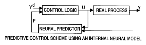
The overall control scheme used is best illustrated in Figure 12. When the
cell is nearing
an anode effect its behavior can be described in different ways depending to a
large extent on the
way the resistance of the gas layer at the anode-bath interface evolves. For
illustrative purpose
three typical states of the cell are considered.
These states are represented, respectively, by curves (a), (b) and (c) in
Figure 13. They
correspond to three different expressions used in the simulator to describe
resistance of the gas
layer forming under the anode-bath interface, which implies for the cell three
dynamic
approaches, and three different approaches of the anodic effect. In the case
of state 1, the
function used is of a very pronounced exponential shape, given by the
following equation:
(S)
Rga, = aQerp(ba(ca - c))
CA 02230882 1998-03-02
- In the case of state 2, the function is also exponential, but more moderate.
It is given by the
following equation:
Rya: =aie~p(bI(cl -c))"a-erp(b-(c3-c)) (()
State 3 of the cell is represented by the parabola functiori given by the
following equation:
Rya- = a3~- ' b3~ ~3 (7)
Parameters ai , bi , ci determine the speed and manner by which the anodic
effect is approached.
Variable c represents the concentration in the aluminum oxide bath.
By acting on the limits of the decision criteria applied by the standard
control logic to
trigger and maintain high-frequency feeding, the cell was overfed with alumina
for three
consecutive hours. The deadband was widened to four times its usual width in
order to avoid the
occurrence of anode adjustments. The cell thus enriched to nearly 4% (instead
of the usual 2 to
3%) was subsequently submitted to underfeeding (feeding reduced to 50%) to
induce anode
effect. During underfeeding the limits of decision criteria of the standard
control logic were
changed so as to avoid the triggering of high-frequency feeding (overfeeding).
Anodic Effects Owing to Random Disturbances
The cell, in each of its three states, is ordered in a first series of
simulations by the initial
control logic (standard logic). In a second series of simulations, the neural
prediction models of
the decision variable are integrated into the standard logic to produce
"neural logic." In each
test, to simulate variations in the property of aluminum oxide, two different
quantities of
aluminum oxide were injected by dumps, following a decision of the control
logic in operation.
These values are respectively equal to the nominal value of the simulator (Q =
3.0 kg/dump), or a
reduced value (Q = 2.4 kg/dump) or (Q = 2.25 kg/dump) to induce anodic
effects. To compare
33
CA 02230882 1998-03-02
the two control versions, the average concentration of aluminum oxide (cp
[%]), the power
consumed by the cell (Ptot [kW]), and the number of anodic effects occurnng
during the
simulation were selected as performance indices.
State 1 Cell with a Steep Exponential Curve Shape
Figure 14 (a) shows a typical example of a simulation of a cell in standard
control. The
first control variable is the feed flow of aluminum oxide represented by the
variable F R [kg/h].
The resistance of the cell R[~S2] constitutes the variable to be controlled.
The anode-cathode
distance, resulting from an anode movement is represented by the variable
D[cm], constitutes the
second control variable. Variables c[%] and F A [kg] represent, respectively,
the concentration
of the aluminum oxide bath and the amount of aluminum produced.
Table (5) summarizes the results over a period of 24 hours of simulation when
the two
logics were applied to the cell in state 1, under nominal (3.0 kg/dump) and
reduced (2.4
kg/dump) supplies. Under the nominal supply range, the two control iogics were
successful in
avoiding anodic effects and gave similar performances as shown in Figures 14
(a) and (b). Under
the two control modes, the cell consumes almost the same amount of energy and
operates under
similar average concentrations. With the reduced supply range, the cell
controlled by the
standard logic is affected by a wave of eight anodic effects, while only one
appears under the
control of neural logic Figures 15 (a) and (b). The energy consumed by the
cell, under standard
control, is high because of the series of anodic effects. A suppression of the
anodic effects is
done automatically by the control logic, by activating ranges of over-supply,
and executing a
series of movements of the anodes. The anodic effect which appears under the
neural control is,
therefore, a consequence of the initial states and the very pronounced
exponential shape (Figure
34
CA 02230882 1998-03-02
13) of the expression of formation of gas under the anode-bath interface, and
not a characteristic
of the dynamics of the cell controlled by neural logic. The speed with which
the anodic effect
appears does not allow time for the neural model to adapt its weights with
regard to the dynamics
of the system.
Table 5: Cell in State 1: Comparison Between the Standard and Neural lagics
with
Nominal and Reduced Supply Dosages.
Supply Control logicc~ Ptot N~ber of Time
[%] [k~ anodic effects[h]
nominal standard 2.38 763.33 0 24
(3.0 kg/dump)
neuron 2.52 761.67 0 24
reduced standard 2.26 901.94 8 24
(2.4 kg/dump)
neuron 2.25 781.39 1 24
State 2 Cell with a Smoother Exponential Curve Shape
This cell corresponds to Curve 2 of Figure 13, which is less steep than Curve
1. Table 6
summarizes the simulation results. Here again, when the cell undergoes nominal
feeding, the
two control logics offer essentially the same performance during the 24-hour
simulation. But
under reduced feeding, as can be seen from Figures 16 (a) and (b), the
standard logic cannot
prevent the anode effects whereas the neural logic can. With the standard
logic, two anode
effects occur within the first 10 hours of simulation. The simulation was
ended after 10 hours
instead of the usual 24 because of numerical overflow after two anode effects,
however this was
sufficient to prove the point. The neural logic-controlled cell operates with
a low value of the
CA 02230882 1998-03-02
._
mean concentration (2.08%) and yet succeeds in preventing the anode effects;
this illustrates the
robustness of the neuron predictive control scheme. Due to the moderate
steepness of the
characteristic curve (Figure 13(b)) as compared to that of the cell state in
(1), even the first anode
effect did not occur. These data illustrate the surprising result that the
power consumption is
lower when the cell is under neural control logic. Finally, an average
concentration is not
calculated for the 10-hour simulations, because after removing the first 1 to
2 hours to discard the
effect of initial conditions, the remaining time length is not sufficient to
yield a representative
mean value.
Table 6: Cell in state 2: Comparison Between the Standard and Neural logics
with
Nominal and Reduced Supply Dosages
Supply Control logiccp Ptot N~ber of Time
[%] [kW] anodic effects[h]
nominal standard 2.26 802.78 0 24
(3.0 kg/dump)
neuron 2.39 799.17 0 24
reduced standard - 883.38 2 10
(2.4 kg/dump)
neuron 2.08 796.97 0 24
State 3 Cell with a Parabolic Curve Shape
Curve 3 of Figure 13 applies. Table 7 shows that under nominal feeding (3.0
kg/dump)
both control logics yield similar performances over the 24-hour simulation
period, without anode
effects. The power consumptions and the average concentrations are similar
under both control
logics. Under reduced feeding (2.25 kg/dump) in the standard logic-controlled
cell two anode
36
CA 02230882 1998-03-02
effects occur within the first 10 hours of simulation, whereas the neural
logic-controlled cell
operates for 24 hours without anode effect. The reason for reducing the
feeding to 2.25 kg/dump
(instead of 2.4 kg/dump as previously) was to deliberately induce anode
effects in the case of
standard control logic. Also in this case, the simulation was ended after 10
hours to avoid
numerical overflow. The neural logic-controlled cell operates with a low value
of mean
concentration (2.19%), and consumes less power than the standard logic-
controlled cell. The
simulation results are displayed in Figures 17 (a) and (b) and Table 7.
Table 7: Cell in State 3: Comparison Between the Standard and Neural logic~
with
Nominal and Reduced Supply Dosages
Supply Control logicc~ Ptot Nmnber of Time
[%] ~~] anodic effects[h]
nominal standard 2.99 786.24 0 24
(3.0 kgJdump) _
neuron 3.09 785.89 0 24
reduced standard - 873.30 2 10
(2.25 kg/dump) "
neuron 2.19 790.60 0 24
This study shows that a neuron prediction contributes to the improvement of
the control
logic performance while avoiding anodic effects. This leads to a decrease in
energy
consumption, a better stability of the cell, and, therefore, an increase in
its yield. The frequency
of the anodic effects is decreased while operating on reasonable average
concentrations.
37
CA 02230882 1998-03-02
The nominal frequency of point-feeding is readily obtained by dividing the
nominal
alumina consumption of the cell by the fixed amount of alumina injected per
dump. A frequency
higher than the nominal value results in overfeeding, a lower frequency causes
underfeeding. A
feeding strategy can be based on varying the frequency and the duration of the
overfeeding and
the underfeeding periods. In the following set of simulations, frequency and
duration of feeding
are gradually reduced to induce the anode effect.
State I - Cell with a Steep Exponential Curve Shape
Figures 18 (a), and (b) show the simulation results from a State 1 cell under
standard and
neural control logics, respectively. In the former, seven anode effects occur
within a 24-hour
simulation period whereas in the latter, only the first anode effect occurs.
This occurrence of the
first anode effect is due to reasons already mentioned. Also, for the neural
logic-controlled cell,
the average concentration is slightly lower and the power consumption
decreases appreciably, as
shown in Table 8.
Table 8: Comparing Standard and Neural Control Logics, for a
State 1 Cell Under Reduced Feeding Frequency and Feeding Duration
Control Logic Cp[%] Ptot Number of Time [h]
anode
[kW] effects
standard 2.44 890.49 7 24
neural 2.21 780.14 1 24
State 2 - Cell with a Smoother Exponential Curve Shape
The standard logic-controlled cell shows two anode effects in the first 10-
hour simulation
period, as shown in Figure 19 (a). In Figure 19 (b) the neural logic-
controlled cell has no anode
38
CA 02230882 1998-03-02
effect. This latter cell also shows a low average concentration and consumes
less power, as
shown in Table 9.
Table 9: Comparing Standard and Neural Control Logics, for a State 2 Cell
Under Reduced Feeding Frequency and Feeding Duration
Control Logic Cp[%] Ptot Number of Time
anode
[kW] effects [h]
standard - 8 81.70 2 10
neural 1.8 8 800.76 0 24
The fact that the cell displays a stable operation at a low concentration is a
sign of the robustness
of the neural control scheme.
State 3 - Cell with a Parabolic Curve Shape
Figure 20 (a) shows the results from a State 3 cell under standard control
logic,
displaying one anode effect. The cell was next simulated under neural control
logic, and results
showed that in this case, even neural control logic could not avoid the anode
effect. This is
believed to result from a combination of the following two reasons. First, the
weights of the
neural networks were obtained through previous learning based on data taken
from cells whose
characteristic curves were exponential (Curves 1 and 2 of Figure 13), whereas
in the present case
the characteristic curve is parabolic (Curve 3 of Figure 13). Also, the
varying of feeding
frequency and feeding duration per se constitutes a change in the present
control logic as
compared to the previous control logic (in which the amount of alumina
injected per dump is
varied). The combined effect of the two changes, one in the cell state and the
other in the control
logic, results in new dynamics to which the neural networks must learn to
adapt themselves, and
to do so additional real-time learning is required.
39
CA 02230882 1998-03-02
_.
During this additional learning, the weights are adapted on-line until an
anode effect is
detected. The last weight values are saved and used in the subsequent
simulation. This process
is iterated until the anode effect disappears. In so doing, it took a total of
nine simulations to
allow the neural network to learn the new cell 'dynamics. The cell under
neural control logic can
then avoid all anode effects during a 24-hour simulation, as shown in Figure
20 (b). Also, Table
shows that under neural control logic, the cell operates at a near-optimal
concentration of
alumina, and consumes less power than under standard control logic.
Table 10: Comparing Standard and Neural Control Logics with Additional
Learning,
for a State 3 Cell Under Reduced Feeding Frequency and Feeding Duration
Control LogicC~[%] Ptot Number of anodeTime [h)
[kW] effects
standard 2.30 806.33 1 24
neural 2.56 788.42 0 24
~''~ntr~~ ~f the Concentration Based on the Recognition of the States
To be efficient, the control of alumina feeding of the electrolytic cell must
be based on
cell resistance, alumina concentration and cell state. Most control schemes
now in use are based
on cell resistance only, and thus constitute an open-loop control that lacks
robustness because
their decision criteria are not explicitly tied to concentration or cell
state. This results in the cell
operating at sub-optimal conditions, diminishing cell efficiency. An optimal
operation requires
the knowledge of alumina concentration and an adjustment of the decision
criteria as a function
of alumina concentration. In this invention, a LVQ-type neural network was
built and trained to
recognize the cell state. Knowing the state of the cell and its resistance,
alumina concentration
can be estimated using predetermined regression functions. The decision
criteria for the control
CA 02230882 1998-03-02
logic are then consequently adapted, and a closed-loop scheme is obtained.
With the cell control
thus structured, the cell can operate at or near optimal conditions and
concentrations
independently of its state. This flexible and intelligent character of the
neural control of the
invention provides a considerable advantage as compared to the standard
control.
The adaptation procedure of the decision criteria of the control logic is the
following:
~ From the characteristic curves corresponding to each cell state, determining
the regression
function giving the concentration as function of cell resistance.
~ Training a neural network of the Learning Vector Quantization (LVQ) type, to
recognize the
present state of the cell, based on its characteristic curve.
~ Knowing the cell's present state and its resistance, estimating the
concentration value using
the corresponding regression function.
~ From a predetermined register, choosing the decision criteria to be applied.
The control scheme is not dependent on knowledge of a precise knowledge of the
concentration,
but rather the recognition of the present state of the cell and of its degree
of richness or poorness
in alumina.
Determination of Regression Fu_n_ction for >;ach Cell State
Starting with each of the three cell states described previously, the cell
controlled is
simulated by its standard control logic and undergoing an overfeeding period
followed by
underfeeding. The overfeeding period was made long enough to allow the
concentration values
to cover the whole range of interest. The underfeeding period was also
maintained long enough
to bring the cell into an anode effect. The deadband was widened to avoid
anode movements.
Deadband is the tolerance zone of the cell resistance value within which a
resistance variation
does not result in an anode adjustment.
41
CA 02230882 2004-O1-29
From the data obtained by simulation, a regression function is determined
giving the
concentration as function of the cell resistance for each of the three cell
states. The following
functions are obtained:
c = a°log(R-a~)+a2 (
c = b° log (R - b,)/bz) + b3 log ((R-b4)/bs) + bb (9)
c=+ -(RI c, +Cz)+C3
( 10)
The variables c and R represent the concentration and the cell resistance
respectively. The
parameters a;, b~, ck are identified through the least square method. On
Figure 21, for each cell
state, the smooth lines show the simulation data and the asterisks give the
regression function
values. Note that for the case of State 3 corresponding to Eq. (10), in t;ie
simulation as well as in
the real physical process, the maximum alumina concentration is about 4% (see
Figure 21); the
regression function of Eq. (10) yields concentrations above that value, but
these have been
ignored.
State Recopyitic~n bX j,~VQ, Network
During each control cycle, the pattern presented to the neural network belongs
to one of
three classes representing, respectively, states 1, 2 and 3 of the cell. This
results in the choice of
a supervised classification algorithm, in the preferred embodiment, a "LVQ"-
type of neural
network (Learning Vector Quantization). The learning of the network is done
"oil line," because
the categories foamed during the learning remain stable, but the prepuation of
the pattern to be
presented at each control cycle is done in real time.
42
CA 02230882 1998-03-02
The LVQ network model is a model made of two layers, an input layer that
stores the
pattern and an output layer that classifies it. The basic algorithm for this
program is well known
in the art. In this model, the two layers are completely interconnected as
shown in Fig. 22. The
output layer is organized to form a topological map of the input patterns. It
is generally
represented by a two-dimensional table where the adjacent neurons within a
given neighborhood
share the similar properties of the input patterns.
The LVQ network model is based on supervised learning. The space formed by the
input
vectors (patterns) is split into regions, each represented by a reference
pattern. The class to which
each pattern belongs is known a priori, and this is what makes the learning
program a supervised
one. One suitable learning program for this invention comprises the basic
algorithm as will as a
weight adaptation algorithm based on the rule of competitive learning in which
only the weights
of the neuron with the highest level of activation are adapted.
In this invention, we have trained and validated an LVQ model network to
recognize the
present state of the cell using the same input vector used by the neuro-
predictor model.
In a first series of simulations, the cell, in each of its three states and
under the control of
its standard control logic, is simulated. In a second series, the neural model
for state recognition
is integrated into the standard logic, and the decision criteria are changed
to fit the needs of each
cell state. Each simulation is carried out over a 24-hour period. The standard
control logic
activates the overfeeding of the cell if 8R > 8R~ or if DR > ~R~,
independently of the value of the
concentration c; in fact, the latter is not even known to the control logic.
In other words, for the
standard control logic the nominal critical values of the decision variables
are held fixed at 8R~
43
CA 02230882 1998-03-02
and ORS. With a neural control logic that can recognize the cell state, these
critical values for
decision, instead of being held rigid, can be modified for each of the cell
states recognized. Note
that the numerical values of 8Rc and ~R~ - a fraction of a ~SZ each - may vary
from one
facility to the next, and their knowledge is not required for the
comprehension of the concepts
conveyed by this text.
Control of Cell in State 1
For the purpose of comparing the neural logic with the standard logic, the
following
modified decision criteria for activating the overfeeding of the cell is
applied to the former logic:
if c < 1.8 8Rc ~ 0.6 BRA, ~ ~ ~R~
if 1.8<_c52.0 BRc~ BRA, ~~~ (11)
if c > 2.0 8Rc ~ 10 BRA, ~ ~ DR
These constraints stipulate that the neural logic operates identically to the
standard logic for
concentrations between 1.8% and 2.0%, but near an anode effect, when the
concentration goes
below 1.8%, the criterion on 8R~ is tightened (8Rc ~ 0.6 8R~). On the other
hand, when the
concentration goes above 2.0%, the criterion on 8R~ is considerably relaxed
(SR~ ~ 10 8R~) to
avoid the activation of overfeeding.
The conditions of decision criteria set 11 force the cell to operate at low
concentrations as
shown in Table 11. Under neural control, the cell, on the one hand operates at
an average
alumina concentration lower than the one obtained with standard logic, and on
the other hand,
succeeds in operating without anode effects at a minimal alumina concentration
2.083%. Figure
23 shows that the slope of resistance controlled by neural logic, band (lvq
(la)), is larger than the
44
CA 02230882 2004-O1-29
one obtained with standard logic. In fact, by operating at low concentrations,
between 2.083%
and 2.275%, the cell is more sensitive, and, therefore, the control is
improved.
Each point on Figure 23 represents a pair of resistance and concentration
values
prevailing at sampling instant. The data point agglomeration is the result of
alternating bet<veen
the over-supply and under-supply ranges. This occurrence leads to a cyclical
character,
oscillations between two limit values, of the resistance and concentration.
Because of the very
marked exponential shape of the curve which characterizes this state, two
areas of operation can
be distinguished between: one corresponding to standard control and the other
to the neural
control.
Control of Cell in State 2.
For illustrative purpose the following decision criteria are first imposed to
the neural
logic:
if c < 2.4 8Rc ~ 0.4 8R~, AR° ~ 0.25 ~
if 2.4 ~ c <_ 2.8 8Rc ~ 0.6 BR~, ARC ~ 0.50 ARC (12)
if c > 2.8 8Rc ~ 0.8 BR~, ~R~ ~ 0.75 ARC
The above criteria stipulate three pairs of critical values for three
different ranges of
concentrations. Note that for all three ranges, overfeeding is activated for
critical values lower
than those applied to the standard logic. As a result, and this can be seen
from the middle part of
Table 1 I at line Ivq (2a), the cell operates at an average concentration
higher than that of the
standard control. To bring the cell to operate at a lower concentration, the
neural logic is now
submitted to the following criteria:
CA 02230882 2004-O1-29
if ~ < 2.o sRc ~ 0.6 sR~, eR~ ~ o.so eR~
if 2.0 < c 5 2.4 sRc ~ BRA, eR° ~ 1.25 eR~ (13)
if c > 2.4 sRc ~ 10 sR°, eR° ~ 1.50 eR~
It can be seen on Table 11 at line lvq (2b), that under neural control, with
the above
criteria the cell operates without anode effect with a minimum concentration
of 1.828%, and an
average concentration of 1.972%, which is lower than that obtained with the
standard logic.
Table 11: Comparison Between Standard Control and Neural
control with Cell State Recognition Madel
Cell State Control LogicCm;"[%) Cm~[%) Cp[%)
1 standard 2.236 2.410 2.318
neuron lvq 2.083 2.275 2.181
(1 a)
2 standard 1.967 2.262 2.166
neuron lvq 2.167 2.318 2.239
(2a)
neuron lvq 1.828 2.131 1.972 .
(2b)
3 standard 2.826 3.038 2.940
neuron lvq 2:857 3.118 3.011
(3a)
neuron lvq 2.476 2.716 2.s88
(3b)
neuron Ivq 1.96s 2.s21 2.169
(3c)
46
CA 02230882 2004-O1-29
Figure 24 shows that when the cell operates at low concentrations - see the
band
identifed as Ivq (2b)-the slope of the characteristic curve is noticeably
steeper than in the case
of higher concentrations - see band lvq (2a). Indeed, when operating at low
concentrations
between 1.828% and 2.131%, the cell is more sensitive and a better control is
obtained.
However, in this zone the control logic generates more anode movements, which
result in sudden
changes, therefore discontinuities, in the cell resistance. This translates
into the discontinuities
(the white strips dividing the band) observed on the band identified as lvq
(2b}. Note that bands
lvq (2a) and lvq (2b) of Figure 24 are generated by the decision criteria (12)
and (13)
respectively.
Because of the moderate exponential shape of the curve characterizing this
state, three
areas of operation can be distinguished: standard, lvq(2a} and lvq(2b) - see
Figure 24.
Control of Cell in State 3
The three following sets of decision criteria are imposed to the neuron-
controlled cell
successively. This is to allow the cell to operate at decreasing concentration
levels.
if c < 2.0 8Rc ~ 0.6 BR~, eR~ ~ 0.50 eR~
if 2.0 S c <_ 3.0 8Rc ~ 0.6 BRA, eR~ ~ 0.75 eR~ (14)
if c > 3.0 8Rc ~ BRA, eR~ ~ eR~
if c < 1.8 8Rc ~ 0.6 BR~, eR° ~ eR~
if .1.8 _< c _< 2.0 SRc ~ BR~, eR~ ~ eR° (15)
if c > 2.0 8Rc ~ 10 BR~, eR° ~ eR~
47
CA 02230882 2004-O1-29
if c < 1.g sRc ~ 0.6 sR~, oR~ ~ eR~
if 1.85c<2.0 sRc~2.08R~, ~~ 1.5~ (16)
if c > 2.0 8Rc ~ 10 BR~, ~R~ ~ 2.0 ORS
The above criteria amount to imposing critical values below or equal to their
nominal
values for high concentrations (Eq. (14)), and increasing them gradually for
lower
concentrations. The last part of Table 11 summarizes the simulation results.
The decision
criteria ( 14), ( 1 S) and ( 16) enable the cell under neural control to
operate at average
concentrations of 3.011%, 2.588% and 2.169% respectively. Criteria (16)
results in the cell
operating without anode effect at a minimum concentration of 1.965% whereas
for the standard
control logic it is 2.826%. Similarly to the preceding cases, Figure 25 shows
that for lower
concentrations, the sensitivity of the cell resistance increases and as a
consequence, the quality of
cell control improves. The bands identified as Ivq (3a), lvq (3b), Ivq (3c) of
Figure 25 are
generated by the criteria (14), (15) and (16) respectively. In this case, due
to the parabolic form
of the characteristic curve (Figure 13) four operation zones can be clearly
recognized on Figure
25: standard, lvq (3a), Ivq (3b) and Ivq (3c).
According to the invention, by adding a neural model for the recognition of
the cell's
state, a close-loop structure, flexible and intelligent, can be given to the
standard contmI logic.
Feeding of the cell is no longer modulated merely as function of the
variations in cell resistance
but also as function of alumina concentration and cell state.
Cell state depends on a number of parameters describing the operational
conditions of the
cell. Among the three typical cell states chosen for study in Figure 13, one
could be seen as the
48
CA 02230882 1998-03-02
normal state (State 2) whereas the other two could be seen as cell conditions
drifting in two
opposite directions. Table 11 shows that under standard logic, the normal cell
operates at an
average concentration of 2.156%. The latter increases to 2.318% and 2.940% in
the other two
cases. Thus, for cell states other than normal, the standard logic tends to
"play it safe" by
operating at higher concentrations in order to steer clear from anode effects.
This behavior of the
standard logic is quite understandable when one considers that, as often
confirmed by cell
operators, about half of the anode effects occur due to poor alumina
feedstock. This precaution
can be removed when the control logic is reinforced by a state recognition
model. A code book
of decision criteria can be elaborated to cover all the typical cell states
and the concentration
values. The state recognition model, combined with the code book of decision
criteria, is-then
incorporated in the control logic to enable it to operate near an optimal
regime whatever the cell
state happens to be.
Thus, by giving to the control logic a close-loop structure through cell state
recognition,
better cell control can be achieved due to the knowledge of the cell state and
the alumina
concentration. The improvement appears evident when such a control scheme is
compared with
the one in which operators control cell feeding using the decision criteria
based on cell resistance
alone, without the knowledge of concentration. Trying to control the
concentration while not
knowing the present value of concentration is indeed a delicate situation.
With an open-loop
structure, large disturbances can cause the cell to drift away from its
nc.~minal state and operate at
concentrations either too low or too high, potentially leading to anode
effects or sludge
formation, respectively. This shows the importance of recognizing the present
operational state
of the cell, and therefore recognizing the applicable characteristic curve
(Figure 13), so that a
49
CA 02230882 1998-03-02
concentration value of the cell could be estimated from its resistance. The
previously rigid
decision criteria 8R~ and ORS can then be adapted so as to avoid activating
the overfeeding when
the cell is in the alumina-rich zone of the curve, and on the other hand,
these criteria can be
tightened as the cell moves toward the alumina-poor zone. Better control may
result in better
cell stability, lower power consumption, higher productivity and longer cell
life.
It should be understood that various changes and modifications to the
preferred
embodiment described herein will be apparent to those skilled in the art. Such
changes and
modifications can be made without departing from the spirit and scope of the
present invention
and without diminishing its attendant advantages. It is intended that such
changes and
modifications be within the scope of the claims.
s0