Note: Descriptions are shown in the official language in which they were submitted.
CA 02331775 2000-11-06
WO 00/48109 PCT/US00/03594
SYSTEM AND METHOD FOR
AN AUTOMATED EXCHANGE
CLAIM OF PRIORITY
This application claims the benefit of priority to U.S. Provisional
Application No.
60/119,888, filed February 12, 1999.
TECHNICAL FIELD
This invention relates generally to trading markets and, more particularly, to
automated methods and systems for trading items in a combined value exchange.
BACKGROUND
An investor often holds a portfolio containing a mixture of types of tradable
items,
such as securities (e.g., stocks, bonds, futures), pollution credits, power
resources,
commodities, resource allocations, etc. The particular mixture gives the
portfolio a variety of
properties, such as yield and long-term stability. Typically, the investor
structures trades so
that these properties are maintained or improved. Maintaining or improving the
properties
often means that the investor wants to trade several different types of items
in each trade.
Such a market is known as a combined value trading market or a combinatorial
exchange.
~5 As an example, the traditional bond market operates by bilateral
transactions in which
each transaction is for one type of bond. To trade several types of bonds, an
investor makes a
series of bilateral transactions with different investors or brokers, each
transaction being for a
portion of the trading goal. Since the trade progresses through a series of
transactions, the
investor takes a new contractual risk at each step without the assurance that
the investor will
2o finally achieve a defined trading goal.
The series of transactions involves a second risk, because information is
disclosed at
each transaction. Information from earlier transactions alerts other market
traders to the
investor's goals. By making a series of transactions, the investor risks less
favorable deals
from later traders who may adjust their trading prices based on the previously
disclosed
25 information.
-1-
CA 02331775 2000-11-06
WO 00/48109 PCT/US00/03594
To avoid adverse market consequences from information disclosure, an investor
frequently hedges bid and/or asking prices to hide the investor's true trading
goal. The
investor offers to trade at prices below the maximum price at which the
investor is willing to
buy and above the minimum price at which the investor is willing to sell.
Hedging deprives
other investors of information but is generally used in an attempt to produce
better prices for
the investor. Unfortunately, hedging also lowers the probability that each
transaction will be
consummated.
For complex mixtures of trading items, the probability that a trader can
achieve a
desired trading mixture decreases rapidly. Hedging further frustrates
prospects for obtaining
complicated mixtures by a series of separate bilateral transactions for single
items.
The present invention is directed to reducing or overcoming the effects of one
or
more of the problems set forth above.
SUMMARY
The invention provides a system, computerized method, and computer program for
~5 operating automated one- or two-sided combinatorial exchanges for trading
items. Functions
or steps of the invention include receiving any of a plurality of orders (a
"package" that may
include logically grouped items) offering to sell items, a package of orders
offering to buy
items, and a package of orders offering to buy and sell items. The method
includes the
principal steps of allocating trading quantities of items to a portion of the
orders, and
20 assigning trading prices for each item allocated a trading° quantity
in an order.
In various embodiments, at least one of the orders is selected from a group
consisting
of a proportional order, an indifferent order, and a complex order. In various
embodiments,
the items traded are selected from a group consisting of securities,
commodities, property
rights, contracts, futures, etc.
25 In one aspect, the invention includes a computerized method of operating an
automated market for trading items, including receiving a plurality of orders
offering to sell
items and a plurality of orders offering to buy items, at least one of the
orders offering to
trade a plurality of types of items; allocating trading quantities of items to
a portion of the
orders, the trading quantities satisfying trading constraints imposed by the
orders; assigning
-2-
CA 02331775 2000-11-06
WO 00/48109 PCT/US00/03594
trading prices to each order for each item therein allocated a nonzero trading
quantity using
at least a direct accommodation algorithm; and outputting information
indicative of the
allocated trading quantities and assigned trading prices.
In another aspect, the invention includes a computerized method of operating
an
automated market for trading items, including receiving a plurality of orders
offering to sell
items and a plurality of orders offering to buy items, at least one of the
orders being an
indifferent order offering to trade between a selection of different items
among a plurality of
types of items; allocating trading quantities of items to a portion of the
orders, the trading
quantities satisfying trading constraints imposed by the orders; assigning
trading prices to
each order for each item therein allocated a nonzero trading quantity; and
outputting
information indicative of the allocated trading quantities and assigned
trading prices.
In another aspect, the invention includes a computerized method of operating
an
automated market for trading items, including receiving a plurality of orders
offering to sell
items and a plurality of orders offering to buy items, at least one of the
orders offering to
t5 trade a plurality of types of items; allocating trading quantities of items
to a portion of the
orders, the trading quantities satisfying trading constraints imposed by the
orders; assigning
trading prices to each order for each item therein allocated a nonzero trading
quantity using a
plurality of pricing paths; and outputting information indicative of the
allocated trading
quantities and assigned trading prices.
2o In another aspect, the invention includes a computerized method of
operating an
automated market for trading items, including receiving a plurality of orders
offering to sell
items and a plurality of orders offering to buy items from a plurality of
traders, at least one of
the orders offering to trade a plurality of types of items; allocating trading
quantities of items
to a portion of the orders, the trading quantities satisfying trading
constraints imposed by the
2s orders; assigning trading prices to each order for each item therein
allocated a nonzero
trading quantity; re-pricing each order of a trading entity having a per unit
surplus value by
redistributing such per unit surplus value to other units of such order; and
outputting
information indicative of the allocated trading quantities and assigned
trading prices.
In another aspect, the invention includes a computerized method of operating
an
3o automated market for trading items, including receiving a plurality of
orders offering to sell
-3-
CA 02331775 2000-11-06
WO 00/48109 PCT/US00/03594
items and a plurality of orders offering to buy items, at least one of the
orders being selected
from a group consisting of a proportional order, a relaxed proportional order,
and a complex
order; allocating trading quantities of items to a portion of the orders using
a method to
increase a total market gain from trading, the trading quantities satisfying
trading constraints
imposed by the orders; assigning trading prices to each order for each item
therein allocated a
nonzero trading quantity; and outputting information indicative of the
allocated trading
quantities and assigned trading prices.
The embodiments include computerized systems and program storage media
encoding executable programs for performing the above-described methods.
1o The details of one or more embodiments of the invention are set forth in
the accompa-
nying drawings and the description below. Other features, objects, and
advantages of the
invention will be apparent from the description and drawings, and from the
claims.
DESCRIPTION OF DRAWINGS
FIG. 1 shows a system for trading a class of items.
~5 FIG. 2 is a flow chart illustrating a method for trading items in a call
market.
FIG. 3 graphically represents two exemplary simple orders.
FIG. 4A graphically represents an exemplary proportional order.
FIG. 4B graphically represents an exemplary relaxed proportional order.
FIG. 5 graphically represents an exemplary indifferent order.
2o FIG. 6 is a flow chart illustrating a method for allocating trading
quantities of items to
orders according to the method of FIG. 2.
FIG. 7 is a flow chart for a method of eliminating orders with low
probabilities of
trading according to the method of FIG. 6.
FIG. 8 graphically illustrates allocation and pricing of trading items in a
single price
25 call market.
FIG. 9 is a flow chart illustrating a method of separating orders into
partitions to
optimize potentials for intra-partition trades.
FIG. 10 is a flow chart illustrating a method of allocating trading quantities
according
to the method of FIG. 9.
-4-
CA 02331775 2000-11-06
WO 00/48109 PCT/US00/03594
FIG. 11 graphically illustrates how order trading conditions on price restrict
the
market price assigned to trading items.
FIG. 12A is a graph allowing direct accommodation for a trade in a single item
call
market where apportioning of costs to satisfy minimum fill conditions occurs
among trading
orders A-D and F-H.
FIG. I2B is a graph requiring general accommodation for a trade in a single
item call
market where apportioning of costs to satisfy minimum fill conditions occurs
among trading
orders A-D and F-H.
FIG. 13 is a flow chart for a method of pricing previously allocated trading
quantities
of items.
FIG. 14 is a flow chart illustrating a method of ticketing allocated and
priced
quantities of items.
FIG. 15 is a flow chart illustrating a method of assigning trading buys and
sells for
direct ticketing and indirect ticketing, respectively.
~5 FIG. 16 is a flow chart illustrating a method ofmatching up buys and sells
for either
direct or indirect ticketing.
FIG. 17 is a flowchart showing an overview of the processes of a matching
engine
suitable for use in a second embodiment of the invention.
FIGS. 18A, 18B, and 18C are related flowcharts showing details of the
embodiment
2o described in FIG. 17.
Like reference numbers and designations in the various drawings indicate like
elements.
-5-
CA 02331775 2000-11-06
WO 00/48109 PCT/US00/03594
DETAILED DESCRIPTION
Glossary
The detailed description of the embodiments may use the following terms.
Accommodation - The process whereby Marginal Orders that are also Inflexible
Orders
compensate the market for their inflexibility. Accommodating these orders (and
Extra-Marginal
Orders) into the market adds liquidity to the market. Denying an order the
opportunity to
accommodate the market for the order's inflexibility and thus denying that
order the opportunity
to trade, can cause other orders to be also no longer able to trade. Because
of the potential
interconnectedness of the orders and items in the market, it is possible that
the entire trading
session would collapse. This partial or complete collapse of trading robs the
market of liquidity,
which is an undesirable event for all traders in the market.
Allocation - The process of matching buys and sells by volume (observing all
Trading
Conditions for the orders being traded).
All-or-Nothing (AON) - A completely inflexible trade requiring that a trade
meet the
~ 5 maximum requirements of the order, or that nothing in the order trades at
all.
ANDI Logic (AND Indifferent) - This logic is used to force all orders
connected by the
ANDI logic to execute to some extent, or else no order in the group will
execute. Typically, if
any one order cannot execute, then none of the orders executes. However, if an
order has no
special trading conditions on it, that is, the order is fully flexible, then
that order is considered to
2o be executed, even if no item in the order is traded, for purposes of
determining the ANDI logic
execution.
ANDP Logic (AND proportional) - This logic is used to force all orders in the
group to
execute in strict proportion to each other. If the orders cannot be traded in
proportion, then none
of the orders executes. The proportion between orders is measured by the
percent fill of each
2s order.
AND Group - A set of orders and/or groups linked together with AND logic.
Asking Price - The sale price offered by a seller for specified items.
Bid Price - The purchase price offered by a buyer for specified items.
-6-
CA 02331775 2000-11-06
WO 00148109 PCT/US00/03594
Budget Limit - This specifies the maximum desired cash flow for an Indifferent
Order.
The Budget Limit limits the total volume traded by an Indifferent Order. Note
that Proportional
and Relaxed Proportional Orders specify their Budget Limits indirectly through
their Unit Offers
and Maximum Quantities.
Call Period - A period for submitting orders to buy and/or sell items. The
call is the set
of orders received during the call period.
Canonical Order - The most basic form of an order. It is a set of one or more
firm offers
submitted to buy and/or sell items. An order may include trading conditions.
Order types include
Simple Orders, Proportional Orders, Relaxed Proportional Orders, and
Indifferent Orders.
Canonical Orders may be logically connected with other Orders using Inter-
Order Logic to
create Strategies.
Child Order - This is an order that is a member of a Parent Order. A Child
Order may
itself be a Parent Order, with Child Orders beneath it. A Bottom Level Child
is always a
Canonical Order.
~5 Clearance & Settlement-The escrow process used to physically consummate
trades.
Clearing Price (Market Price) - In a call market having a single trading
price, the
clearing price is the calculated price at which those items trade. The
clearing price is determined
by the bid and asking prices of the orders with items trading at the margin
(Marginal Orders).
Combinatorial Trading -- The opportunity to engage in the simultaneous buying
and
2o selling of many combinations of things.
Contra - short for contraposition. The contra of an order to buy an item is an
offer to sell
the item.
Delivery-sized Data File - a performance benchmark set of data consisting of
50,000
orders and 2,000 commodities.
25 Delta - This parameter delineates how far from an ideal proportion line an
order is
allowed to deviate in an attempt to trade. As used, delta specifies the
percent deviation from the
ideal proportion line. Delta is used in conjunction with Relaxed Proportional
Orders.
Direct Ticket - A trading ticket for a trade made directly between the buyer
and seller.
No intermediaries are involved.
CA 02331775 2000-11-06
WO 00/48109 PCT/US00/03594
Execute - An order that meets its minimum Trading Conditions trades or
executes. An
order that meets its maximum Trading Conditions fully executes.
Extra-Marginal Order-An order that is allocated and resides to the right ofthe
Market
Cross. These orders are allocated solely to accommodate an inflexible marginal
order.
Flexibility Parameters - A set of parameters that may be used to describe
ranges of
acceptable trading conditions for an order, such as quantities, total monetary
amounts, and item
compositions. Flexible orders are orders that may be allocated over a wide
range of possible
trades. Inflexible orders are orders that may trade in a very narrow range of
possible conditions.
Flexibility Parameters include Delta, Minimum Fill, Minimum Quantity, and Odd
Lot.
Flexible Order - An order where the trader places minimal limitations on the
degree to
which an order executes. Fully Flexible Order is an order where the trader is
willing to accept
any degree of execution of his order from none to full. The more flexible an
order is, the more
likely it is to trade (provided it specifies competitive unit offers).
Flexibly Allocated, Zero Surplus - FZS. The order is in the Flexible
Allocation, but has
zero surplus. The order may be fully or partially flexibly allocated.
Flexibly Fully Allocated Order - FA. This is an order that trades to its
allocated limits
during the flexible allocation phase.
Flexibly Partially Allocated Order - FPA. This is an order that has traded,
but not to its
allocated limits during the flexible allocation phase.
Flexibly Rejected Order - FR. This is an order that did not trade during the
flexible
allocation phase.
Fully Allocated Order - This is an order that has traded to its maximum
limits.
Gains-from-Trade - This is a calculated value that gives an indication of the
efficiency
of the market, and how much improvement an order achieved over its monetary
trading
conditions. The gain of an item being bought is the value of the bid price
minus the market price,
times the quantity traded. The gain of an item being sold is the value of the
market price minus
the asking price, times the quantity traded. The gain for an entire order is
the sum of the gains of
the items bought and sold therein. The gain for the market as a whole is the
sum of the gains of
all of the orders being traded.
_g_
CA 02331775 2000-11-06
WO 00/48109 PCT/US00/03594
Indifferent Order - An order that allows the trader to benefit from his
willingness to
trade between a selection of different items, where the trader perceives those
items as being
functionally equivalent. For example, if a trader wishes to buy a dozen
muffins and does not care
whether they are banana nut, cranberry, or bran muffins, then an Indifferent
Order allows the
trader to specify all three equivalent muffin types and end up with the best
available mix of the
three muffin types. With Indifferent Orders, the total Trading Quantity is
determined by the
Indifferent Order's budget, and the individual items are not guaranteed to
trade in any particular
ratio. An Indifferent Order must be a pure buy or pure sell.
Indirect Ticket - A trading ticket for a trade in which an intermediary acts
as the buyer
for the seller, and the seller for the buyer. Usually there is a difference in
the buy and sell price
and that is why a Direct Ticket cannot be used. This price differential
requires an intermediary to
act as a clearing agent.
Inflexible Order - An order where the trader places stricter limitations on
the degree to
which his order executes. A completely inflexible order is an all-or-nothing
(A01~ order. The
less flexible an order is, the less likely it is to trade.
Infra-Marginal Order - An order which is allocated and resides to the left of
the
Market Cross. This order does not trade at or through the cross when a supply
and demand curve
is drawn using the allocated orders.
Inter-order Logic - The ANDI, ANDP, XOR, or KOR logic used to connect orders
into
2o a strategy group.
Item - A commodity to be traded. An item can be any tangible or intangible
thing for
which a property right can be defined.
Item Count/List - The number and identification of the items in an order.
Key Order - The primary (most desired to execute by the trader creating the
group)
order in a KOR group. The Key Order is usually a package order. Generally, the
Key Order is
priced as a more attractive trade than the conglomeration of Minor Orders in a
KOR group.
KOR Logic (Key Order OR) - This logic is used to allow a trader to trade an
entire
package, or to trade as many pieces of a package as possible. The KOR group is
composed of
one Key Order and a series of Minor Orders. The logic is performed such .that
either the Key
3o Order executes, and none of the Minor Orders execute; or the Key Order does
not execute, and at
-9-
CA 02331775 2000-11-06
WO 00/48109 PCTIUS00/03594
least one {perhaps all) of the Minor Orders execute. It is also possible that
neither the Key Order
nor any of the Minor Orders trade. Note that while KOR logic exhibits
similarities to XOR
groups, they are not the same.
Liquidity Providing Strategy - a group of orders ANDed together to bring
additional
volume/liquidity to a market, provided certain price and contra-side volume
requirements are
met.
LP {Linear Program) - A system of linear equations used to model a problem.
Marginal Order - An order that trades at least one item at the Market Cross or
extra-
marginally. Marginal Orders can be single item or package orders. Marginal
orders are useful in
setting the market price for the items being traded.
Market Cross - The point at which the supply and demand curves for an item
meet.
Traditionally in a single item market, all orders to the left of the cross
trade, and no orders to the
right of the cross trade.
Market Prices - The final prices at which various items trade. The market
prices depend
~ 5 upon the item being traded and the orders involved in trading that item.
The market price is the
single price reported or quoted to the world at large. Note, however, that
different orders may
trade the same item at prices different from the market price. These are the
various orders'
Trading Prices. These differences are due to the system accommodating the
rigidity of certain
orders in order to add liquidity to the market as a whole.
2o Maximum Quantity - This specifies the upper limit for the number of units
that an
order is willing to trade of an item.
Minimum Fill - This specifies the minimum degree to which an order executes.
For a
proportional or relaxed proportional order, the Minimum Fill generally applies
to the total
volume traded, but may apply to the Budget Limit. For an Indifferent Order,
the Minimum Fill
25 applies to the Budget Limit.
Minimum Increment - This is the minimum quantity step that an order is willing
to
trade of an item.
Minimum Quantity - This describes the minimum acceptable trading quantity for
an
item in an Indifferent Order. That is, an item must trade at least the Minimum
Quantity in
3o volume, or it will not trade at all.
-10-
CA 02331775 2000-11-06
WO 00/48109 PCT/US00/03594
Minor Orders - The orders representing a less desirable trading mix than the
Key Order.
Typically, Minor Orders are created by making a series of simple orders or
orders of smaller
packages of items using the same items specified in the Key Order. However,
the Minor Orders
can be orders with little or no overlap in items with the Key Order. The
composition of the
Minor Orders is entirely up to the trader.
MIP (Mixed Integer Program) - An LP in which one or more of the variables are
integers.
Natural Decomposition -- The process where a partition of orders can be
cleanly split
into two or more independent groups where none of the groups share any items
in common.
Odd Lot - This describes the minimum residual quantity acceptable in an item
sold by
an Indifferent Order. That is, an item for sale in an order with an Odd Lot
for that item must
trade the Maximum Quantity for that item, or zero quantity, or between the
Minimum Quantity
and (Maximum Quantity - Odd Lot).
OR Group - Shorthand term for XOR Group: a set of Canonical Orders and/or
Order
Groups linked together with XOR Logic.
Order - A set of one or more firm offers submitted to buy and/or sell items.
An order
may include trading conditions. Order types include Simple Orders,
Proportional Orders,
Relaxed Proportional Orders, and Indifferent Orders. Orders may be logically
connected with
other orders to form Strategies.
2o Order Group - Any set of orders linked together with Inter-Order Logic. An
Order
Group may be composed entirely of Canonical Orders, or entirely of Order
Groups, or a mixture
of both.
Order Logic - The Boolean-style logic used to connect two or more orders
together to
create a strategy. The basic logic types are exclusive OR and AND.
2s Order Type - The general character of an order: simple, proportional,
relaxed
proportional, or indifferent.
Package Order - This is the same as a combinatorial order. It is composed of
at least
two items for trading at specified prices per unit traded.
Partition - A group of orders.
-11-
CA 02331775 2000-11-06
WO 00/48109 PCT/US00/03594
Parent Order - Canonical Orders and Order Groups may be nested together, with
no
theoretical limit to the depth of nesting. A Parent Order is an order that
defines which orders are
logically linked together. A Parent Order may have a Parent Order above it. A
Top Level Parent
Order is the order at the top of the nesting hierarchy.
Partially Allocated Order - This is an order that has traded between its
minimum and
maximum limits.
Portfolio - This is a complete group of items or investments held by a trader.
A portfolio
trade occurs when a trader acts to change the composition of his portfolio.
Pricing - The action of determining Market Prices for all Allocated Items in a
Call.
Proportional Order - This is an order offering to trade two or more items in
conjunction. These items are offered to trade in strict quantity ratios
between the items. For
example with a two item order having a ratio of 2:3, for every two units of
item A traded there
must be three units of item B traded; or with a three item order, the three
items might trade in a
ratio of 3:2:17. Any number of items may be included in a proportional order.
A proportional
order may be a pure buy, a pure sell, or a swap order.
Pure Buy Order - An order composed only of items offered for purchase.
Pure Sell Order - An order composed only of items offered for sale.
Relaxed Proportional Order - This order is similar to a proportional order in
that it is
an order offering to trade two or more items in conjunction. However, the
items offered for trade
2o are expected to trade in approximate proportion as opposed to strict
proportion. For example, a
three item order may be offered to trade in an ideal ratio of 3:2:10, but the
trader is willing to
trade in ratios within 10% of the ideal ratios. In this example, the trader is
willing to trade in
ratios of 2.7:2:9, or 3:1.8: I0, and so on over all possible ratio
combinations that are within 10%
of the trader's ideal ratio.
Re-pricing - An action whereby the Gains from Trade for an individual order
are
redistributed equally among all items (units) trading. Normally, the Gains
from Trade are
distributed so that the order as a whole has positive gains, but some items
may have negative
gains when viewed in isolation. With re-pricing, the Gains from Trade are
distributed by re
calculating the Trading Price so that each Item has positive Gains from Trade
relative to the
order's original Unit Offers.
-12-
CA 02331775 2000-11-06
WO 00/48109 PCT/US00/03594
Simple Order - This order is one side of a traditional bilateral trade. There
is a single
item offered for sale or to purchase at a specified price per unit traded.
Standalone Order - This is a Canonical Order that has no Parent Order. That
is, the
order is not logically linked to any other order.
Strategies - Trading strategies are implemented by logically grouping two or
more
orders together in an attempt to achieve a more complex trade sequence. For
example, a trader
may want to execute a liquidity providing strategy. The trader offers to sell
more volume in an
item or a series of items if the trader can get a better price and if there is
additional demand for
the items) at the better price.
1o Swap Order - This is an order in which various items are offered for sale,
and other
items for purchase within a single order.
Thick Item - This is an item where a relatively large number of orders are
offering to
trade the item.
Thin Item - This is an item where a relatively small number of orders are
offering to
trade the item.
Tickets - Bilateral contracts for one item in which a buyer buys and a seller
sells the
same quantity of a traded item at the same price. Tickets are used to
facilitate the integration of a
combinatorial market's results into traditional clearance and settlement
mechanisms.
Trading Conditions - These are conditions imposed on the offers of an order by
the
2o trader. The conditions may set minimum asking prices, maximum bidding
prices, maximum
and/or minimum quantities to trade, item compositions of trades, and logical
relations between
other orders. Trading conditions may be fixed values or set ranges of
acceptable values. Trading
Conditions include Budget Limit, Inter-Order Logic, Item CountlList, Maximum
Quantity,
Minimum Increment, Order Type, and Unit Offer, along with all Flexibility
Parameters.
Trading Price - This is the actual price per unit paid or received by an order
for a
particular item being traded by that order. The trading price for an item in
an order can be
different from the clearing price for that same item in the open market.
Trading Quantity - This is the actual volume trading for an item in an order.
This
number is always less than or equal in magnitude to the Maximum Quantity of
the item.
-13-
CA 02331775 2000-11-06
WO 00/48109 PCT/US00/03594
Unallocated Order -An order that did not trade either because its minimum
acceptable
limits could not be met or other more attractive orders beat it out.
Unit - This is a standard single quantity of volume in an item, e.g., a pound,
a bond, a
lane. Items need not trade in integer units, as some applications may permit
trading a half ton of
an item where Maximum Quantities are normally specified in tons.
Unit Offer - The target bid or ask price that an order presents per unit
volume of item.
XOR Logic (exclusive OR) - This logic is used to force only a single order in
the group
to execute. No more than one order in an XOR group may ever execute.
Your Price - This is the same as Trading Price.
1o Overview of Operational Environment
FIG. 1 shows a system 2 for trading items in a market. The items traded may
belong
to any class of items tradable together on a market, such as securities (e.g.,
stocks, bonds,
futures), pollution credits, power resources, commodities, resource
allocations, etc.
During a preselected call period, the system 2 accepts orders submitted
through client
15 computer tenminals 3-5. The computer terminals 3-5 execute (either directly
or through an
attached server computer) a program for submitting orders to and fox receiving
trading
information from a central processing system 6 {e.g., a server). The trading
information
includes data on previously received orders, e.g., offered buy/sell quantities
and/or prices. A
trader controls the availability of information about the trader's order
(e.g., prices, quantities,
2o etc.) to other traders through commands submitted with the order. The
computer terminals 3-
may execute software providing a graphical user interface (GUI) to submit
orders and
receive trading information and results. One such GUI suitable for trading
bonds is the
BR117GESTATION GUI available from Bridge Information Systems.
The.processing system 6 includes at least one program storage device 7 for
storing
25 software and, preferably, one or more high speed processors 8 for executing
portions of the
program. A plurality of processors 8 may be configured as a loosely or tightly
coupled
parallel processing system. The software program determines trading
quantities, trading
prices, and, optionally, bilateral settlement tickets for the items of each
order through
methods described below.
- 14-
CA 02331775 2000-11-06
WO 00/48109 PCT/US00/03594
The invention may be implemented in hardware or software, or a combination of
both
(e.g., programmable logic arrays). Unless otherwise specified, the algorithms
included as part of
the invention are not inherently related to any particular computer or other
apparatus. In
particular, various general-purpose machines may be used with programs written
in accordance
with the teachings herein, or it may be more convenient to construct more
specialized apparatus
to perform the functions described herein. However, preferably, the invention
is implemented in
one or more computer programs executing on one or more programmable computer
systems each
including at least one processor, at least one data storage system (including
volatile and non-
volatile memory and/or storage elements), at least one input device or port,
and at least one
output device or port. Program code is applied to input data to perform the
functions described
herein and generate output information. The output information is applied to
one or more output
devices, in known fashion.
Each such program may be implemented in any desired computer language
(including
machine, assembly, or high level procedural, logical, or object oriented
programming languages)
~5 to communicate with a computer system. In any case, the language may be a
compiled or
interpreted language.
Each such computer program is preferably stored on a storage media or device
(e.g.,
magnetic, optical, or solid-state media) readable by a general or special
purpose
programmable computer system, for configuring and operating the computer when
the
2o storage media or device is read by the computer system to perform the
functions described
herein. The inventive system may also be considered to be implemented as a
computer-
readable storage medium, configured with a computer program, where the storage
medium so
configured causes a computer system to operate in a specific and predefined
manner to
perform the functions described herein.
25 Overview of Trading System and Method
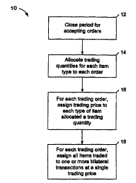
FIG. 2 illustrates an automated method 10 of trading items on a market
according to
one embodiment of the invention. After a predetermined time, the processing
system fi closes
the call period for receiving orders and starts processing the orders
received, i.e., the orders
of the call (step 12). The processing system 6 allocates trading quantities
for each item type
-15-
CA 02331775 2000-11-06
WO 00/48109 PCT/US00/03594
to each received order (step 14). The processing system 6 determines the
trading quantities
using a method that maximizes the overall market gain from the entire set of
trades without
violating trading conditions imposed by orders. The processing system 6 may
allocate zero
trading quantities to some item types in some or all of the orders. Next, the
processing system
6 assigns a trading price to each trading quantity already allocated to an
order (step 16). The
processing system 6 assigns trading prices and quantities so that each trading
order has a
non-negative total gain. The steps of allocating and assigning price may
include creating a
table in the storage device 7. Such a table preferably lists the trading
quantities and prices for
each order without listing which trader will accept the offers in the orders.
Finally, the
processing system 6 determines the identities of the accepting traders and
assigns the trading
quantities to bilateral transactions at a single trading price between
individual offerors (step
18). Optionally, "tickets" (enforceable trading contracts) may be output. More
generally, the
system may simply output a report of matched trades.
For ease of understanding, the remainder of the description will discuss
markets for
~5 trading securities. Nevertheless, the scope of the invention includes any
class of items having
a market for combined value trading.
Order Types
The system 2 and method 10 of FIGS. 1 and 2 can process the following types of
orders: simple orders, proportional orders, relaxed proportional orders, and
indifferent orders.
2o An order may include trading conditions. Each order can include offers
either to buy or to
sell, and some orders can include both simultaneously. Orders may be logically
connected
with other orders to form strategies.
Simple orders are offers to buy or sell one type of security. A simple order
specifies
the item type, the asking or bid price, and a maximum quantity. The offer is
for a buy or a
25 sell according to whether the maximum quantity is positive or negative,
respectively. The
trader's order is a firm offer to trade the specified item subject to
conditions. The trade
quantity cannot exceed the specified maximum, and the price must satisfy the
conditions. For
offers to sell, the price condition is to sell at any price no less than the
asking price. For
offers to buy, the price condition is to buy at any price no greater than the
bid price.
- 16-
CA 02331775 2000-11-06
WO 00/48109 PCT/US00/03594
A simple order includes one flexibility condition expressing the offeror's
flexibility to
trade quantities. The flexibility condition is a minimum fill percentage. The
minimum fill
percentage times the specified maximum quantity is the minimum quantity that
can trade.
The offer is conditioned on an acceptance of, at least, the specified minimum
percentage
times the maximum quantity in the simple order. Of course, the entire order
can be rejected.
FIG. 3 graphically represents two simple orders C and D, made by the same
offeror,
for securities A and B, respectively. Before each trade, the offeror initially
has 500 units of
both security A and security B. In order C, the offeror offers to buy between
S00 and 1,000
units of security A. The solid line between 1000 and 1500 units of security A
and located at
1o the pre-trade 500 units of security B illustrates the order C. Thus, the
maximum trading
quantity for order C is 1,000 units of security A, and the minimum fill is
50%. In order D, the
offeror offers to buy between 250 and S00 units of security B. The solid line
between 750
and 1000 units of security B and located at the pre-trade 500 units of
security A illustrates the
order D. Thus, the maximum trading quantity is 500 units of security B, and
the minimum fill
15 is again 50%.
A proportional order offers to buy and/or sell several types of securities. A
proportional order specifies the types of securities offered, the asking or
bid price for each
type, the maximum quantity to trade for each type, and a mix for the various
types. The
percentage mix fixes the numerical percentages of the various securities
offered. FIG. 4A
2o graphically represents a proportional order using the quantities from FIG
3. Security types A
and B trade in strict proportion, resulting in a straight line S of
permissible trading values.
A relaxed proportional order also has two flexibility parameters. The first
flexibility
parameter is the minimum fill percentage, F. The minimum fill times the sum of
all
maximum quantities offered for each security defines the minimum quantity of
securities
25 upon which the offer is conditioned. The second flexibility parameter, 8,
is a range for the
percentage mix of the individual securities in the order. Alternatively, the
minimum fill for
relaxed proportional orders may be based on a budget limit rather than on
total quantity.
FIG. 4B graphically represents a relaxed proportional order E for a mixture of
the
security types A and B by the crosshatched region E. The order E is an offer
to buy a
3o maximum of up to 1,000 units of security A and up to 500 units of security
B at a mixture of
17-
CA 02331775 2000-11-06
WO 00/48109 PCT/US00/03594
66.67% security A and 33.33 % security B. The dashed line of FIG. 4B labeled
"Mix"
indicates the precise mixture of 66.67% A and 33.33% B values. Given an
initial portfolio
position of 500 units of A and 500 units of B, the order's maximum buy limits
of 1,000 units
of A and 500 units of B would give the offeror a maximum of 1,500 units of A
and 1,000
units of B. These upper limits are indicated by boundaries "Max A" and "Max $"
of the
region E of FIG. 4B. The order E gives the minimum fill constraint F as 50%
and is thus,
conditioned on trading, at least, 750 units of securities A and B together as
indicated by the
boundary line MF in FIG. 4B. Finally, the order E gives the flexibility 8 of
the mixture as
50%. Thus, the order offers to trade any mixture including between 50% less of
security A,
as indicated by boundary L1, to 50% less of security B, as indicated by
boundary L2.
A relaxed proportional order is similar to a proportional order in that it is
an order
offering to trade two or more items in conjunction. However, the items offered
for trade are
expected to trade in approximate proportion as opposed to strict proportion.
For example, a
three-item order may be offered to trade in an ideal ratio of 3:2:10, but the
trader is willing to
~5 trade in ratios within 10% of the ideal ratios. In this example, the trader
is willing to trade in
ratios of 2.7:2:9, or 3:1.8:10, and so on over all possible ratio combinations
that are within
10% of the trader's ideal ratio.
An indifferent order is a unique mufti-security offer conditioned on total
trading
dollar amounts rather than security composition. The offers for the individual
securities of
2o the order are either all buys or all sells. An indifferent order gives the
types of securities
offered, the asking or bid prices for each type as appropriate, the maximum
quantity to trade
for each type, and the maximum dollar amount for the trade.
An indifferent order also has two flexibility parameters. The first
flexibility
parameter, F, gives a minimum fill percentage of the total dollar amount on
which the offer is
25 conditioned. The second flexibility parameter, minQty, specifies a minimum
quantity of each
type of security to trade. The second flexibility parameter must be less than
the smallest of
the specified maximum trading quantities for the various~securities. A sell
order may have a
minimum leftover (odd lot) quantity restriction as well.
FIG. 5 illustrates the allowed trading region "F" of an indifferent order for
a sell.
3o Before the sell, the seller's pre-trade situation is 1,500 units of
security A and 1,250 units of
-18-
CA 02331775 2000-11-06
WO 00/48109 PCT/US00/03594
security B. The trading region F has boundaries "I" and "J" indicating the
respective
maximum sale quantities of 1,000 units of security A and 750 units of security
B. The trading
region F also has boundaries "G" and "H" indicating minimum odd lot quantities
of 125 units
for each of A and B. Finally, the trading region has boundaries "K" and "L"
indicating a
maximum dollar amount to sell of $1,250 and that the minimum fill of the
maximum dollar
amount is 50%. Note that this example is drawn using equal unit offers; the
slopes of
boundaries "K" and "L" will vary at different unit offers. The unit offers for
each item in the
order and the maximum Budget Limit must be known in order to draw "K "; "L" is
a
function of F times the Budget Limit. "K " and "L" will always be parallel to
each other. The
slopes of "K" and "L" are determined by the unit offers for "A" and "B", and
the Budget
Limit. With indifferent orders, it is possible to have one or more of the
items in the order not
trade, while at least one item does trade. This is shown in FIG. 5 by means of
solid line
segment "M" and "N" drawn on the dotted lines outside of boundaries "G" and
"H". The line
segments "M" and "N" are bounded by extensions of boundary "L" out to the
dotted lines
~5 and extensions of boundaries "J" and "I" out to the dotted lines.
Traders can also submit complex orders that group together smaller orders with
OR
and AND logic, examples of which are shown in TABLE 1 below. The OR and AND
logic
correlates acceptance of orders connected by the logic and is preferably
implemented by
additional discrete valued (i.e., integer or binary) order variables.
2o Two types of OR logic can couple orders. The first type is an exclusive OR
(XOR). If
XOR couples two or more orders, the system 2 of FIG. 1 only accepts the one of
the coupled
orders that maximizes the market gain or no order in the group trades at all.
The second type
of OR logic, KOR logic, couples a "key" offer to "minor" offers. The system 2
only accepts
either the key order or a subset of the minor orders or none of the orders
trade. The selection
25 is made to maximize the overall market gain.
There are also two types of AND logic, which either trade all orders coupled
by the
logic or no orders coupled by the logic. For the first type of AND logic,
i.e., AND Indifferent
(ANDI) logic, the system 2 accepts all orders coupled by AND if each order so
coupled at
least partially trades. For the second type of AND logic, i.e., AND
Proportional (ANDP)
- 19-
CA 02331775 2000-11-06
WO 00/48109 PCT/US00/03594
logic, the system 2 accepts orders coupled by the logic if each order so
coupled trades at the
same fill percentage.
TABLE
1
LOGIC ORDER RESULT
A1 XOR A2 Either Al trades or A2 trades, or neither,
but not both
A1 KOR {B1, B2, B3, Either A1 trades or part or all of {Bl,
...} B2, B3, ...} trades, or
none trade
Al AND A2 Either A1 and A2 both trade, or neither
trades
If AND = ANDP Trade only occurs if A 1 and A2 have same
fill
percentage
If AND = ANDI Trade only occurs if A 1 and A2 fill to
any allowed
percentage
{A1 AND AZ} XOR B1 Either A1 and A2 both trade, or B1 trades,
or nothing trades
The various types of intra-order logic among offers may be implemented with
logical
connectors or discrete valued variables. In suitable situations, integer
variables rnay be used.
First Embodiment
A first embodiment of the invention is described in this section. This
embodiment
also provides an overview of the general functions performed by the second
embodiment
described below.
Allocating Trading Quantities
FIG. 6 is a flow chart illustrating one method 14 (corresponding to step 14 of
FIG. 2)
for allocating the trading quantities to orders. First, the processing system
6 determines
which orders have a low probability of trading and marks such orders as non-
trading (step
~5 22). Next, the processing system 6 assigns the remaining orders to separate
partitions by a
method which assigns orders with higher potentials for trading among
themselves to the
same partition (step 24). Next, the processing system 6 finds a separate
trading solution for
each partition (step 26). Each separate solution fixes potential quantities of
securities traded
among the orders of the same partition. To find the separate solutions, the
processing system
20 6 uses a method for separately optimizing the sum of the gains of the
orders of each partition.
-20-
CA 02331775 2000-11-06
WO 00/48109 PCT/US00/03594
Next, the processing system 6 determines whether the step of determining
separate
solutions has used more than an allotted processing time for finding such
solutions (step 27).
If not, the processor finds a new trading solution for the orders found to
trade in step 26, by
globally optimizing the gain (step 28). Then, the new trading solution
determines trading
quantities for the individual orders. If more than the allotted time has been
used, the
processor 6 determines the trading quantities for the individual orders from
the separate
solutions for each partition (step 29).
Eliminating Low-Probability Orders
FIG. 7 illustrates a method 22 (corresponding to step 22 of FIG. 6) of
eliminating
orders with low probabilities to trade. First, the processing system 6
eliminates orders not
satisfying volume conditions on trading quantities (step 32). For example,
such orders
include buys where minimum buy quantities are greater than the total
quantities offered for
sale. Next, the processing system 6 separates each order into suborders for
single security
types (step 34). For the suborders of each security type, the processing
system 6 finds
hypothetical trading quantities and prices that would result if the suborders
formed a call
submitted to a single-price call market for that security where each suborder
is treated as
"fully" flexible (step 36). The hypothetical trading prices are the clearing
prices of these call
markets. Next, the system 6 calculates a hypothetical gain for each order as
the sum of the
gains of the suborders of the order (step 38). Finally, the processing system
6 eliminates
20 orders with gains below a preselected threshold value (step 40). Only the
remaining orders
can trade, i.e., orders having higher potentials to trade.
Within indifferent orders, individual security types can also be eliminated.
Using the
same scoring process within an order, the potential gain contributed to the
order by each
security type is compared to the pre-selected threshold. Those security types
below the
25 threshold are eliminated from the indifferent order.
In some embodiments, the processor 6 performs a second elimination of orders
not
satisfying trading volume conditions after step 40. For the second
elimination, volume
conditions can be fulfilled only through trades with other orders having gains
above the
preselected threshold.
-21 -
CA 02331775 2000-11-06
WO OOI48109 PCT/US00/03594
Single-Price Call Market Algorithm
FIG. 8 is a graph 42 illustrating how the single-price call markets of step 36
in FIG. 7
determine the hypothetical trading quantities and prices the calls of fully
flexible orders. The
orders include offers to buy A-E and offers to sell F-J for a single item at
the order prices and
maximum quantities illustrated in FIG. 8. From left to right, the graph 42
displays offers to
buy A-E and offers to sell F-J with respective bid and asking prices arranged
in decreasing
and increasing orders. Since the marginal orders are fully flexible, orders
and portions
thereof trade if they are to the left of crossing point 44 of the lines
plotting the offers to buy
A-E and offers to sell F-J. Thus, the offers to buy for the highest prices and
to sell for the
lowest prices trade (i.e., orders A-D and F-H). The clearing price is located
in a region 46
between the asking price 48 and the bid price 49 of orders H and D at the
margin of the
trading region. In particular, the call markets of step 36 in FIG. 7 set the
hypothetical trade
price at point 50 halfway between the marginal asking and bid prices 48, 49.
Since the orders
A-J are all fully flexible, the trading orders A-D and F-H trade at a trading
price equal to the
clearing price 50. The trading prices for trading orders A-D and F-H satisfy
trading
conditions, i.e., trading prices 49 are less than the bid prices and greater
than the asking
prices 48.
If the order (demand) and offer (supply) curves do not cross (e.g., only
orders I, J, D,
& E are in the market, but might trade due to combinatorial constraints), the
price is
2o preferably set by taking the average price of the highest buy & lowest
sell.
Assigning Orders to Separate Partitions
FIG. 9 is a flow chart illustrating one method 24 (corresponding to step 24 of
FIG. 6)
of decomposing the orders of the call that remain after step 40 of FIG. 7 into
separate
partitions. The processing system 6 starts the decomposition by constructing a
graph of nodes
25 and arcs (step 53). The graph is a connected set of arcs and nodes in which
each arc connects
one pair of nodes and each node corresponds to a single order. To represent
orders that offer
to trade several securities, a separate arc connects a pair of nodes of the
graph for each type
of security that the corresponding orders can trade. For example, one arc
connects a pair of
-22-
CA 02331775 2000-11-06
WO 00/48109 PCT/US00/03594
nodes for two orders that can trade one type of security, two arcs connect a
pair of nodes for
two orders that can trade two types of securities, etc.
The processing system 6 preferably constructs the graph as a stored data
table. For
example, the table may have rows and columns indexed by nodes or orders. Then,
the
number of arcs connecting a pair of nodes of the graph is indicated in the
table by an integer
stored at the row and column for the two nodes. A graph can also be visualized
as a
connected drawing of the nodes and arcs, as known in the general art of graph
decomposition.
After constructing the graph, the processing system 6 assigns weights to the
nodes
and arcs of the graph (step 54). One way to assign weights is to assign each
of the nodes and
arcs a weight of one. Other ways to assign weights give different weights to
the arcs than to
the nodes.
After assigning weights to the nodes and arcs, the processing system 6 finds
the node
that produces the largest combined weight when combined with another node and
the arcs
connecting the two nodes (step 55). The weight of a combined node is defined
as the sum of
the weights of the original arcs and nodes combined therein. After finding the
pair of nodes
that produces the largest combined weight, the processing system 6 determines
whether the
combined weight is above a preselected threshold value (step 56). If the
combined weight is
not above the threshold value, the processing system 6 combines the two nodes
from step 55
20 (step 57) and then loops back to fmd a new largest node. If the combined
weight is above the
threshold value, the processing system 6 determines whether a remaining third
node exists to
combine with the first node of step 56 (step 58). If no third node exists, the
processing
system 6 separates off the first node as a new partition (step 59). If there
is a third node, the
processing system 6 finds the third node that produces the highest weight when
combined
25 with the first node (step 60). Then, the processing system 6 loops back to
step 56 to
determine whether the new combined weight is above or below preselected
threshold.
The processing system 6 repeats steps 55-60 until the first node with the
largest
below-threshold weight is found. The processing system 6 separates off this
first node as a
separate partition in accordance with the step 59. The method 24 distributes
the various
30 orders into separate partitions for which infra-partition potentials for
trades are increased.
-23-
CA 02331775 2000-11-06
WO 00/48109 PCT/US00/0359~
Optimizing Trading Gains
The processing system 6 handles minimum fill trading conditions by using both
discrete and continuous order-defining variables. For example, a fully
inflexible offer (also
known as All-Or-Nothing or AON) to sell A securities is an offer to sell XA
securities with
X = 0 or 1, i.e., X is a binary integer variable. Partial fill conditions and
logical nesting
conditions also involve integer valued variables. To determine the trading
quantities in the
method 14 of FIG. 6, the processing system 6 optimizes total trading gains
generally
depending on both integer and continuous variables.
FIG. 10 illustrates a method 26 (corresponding to step 26 of FIG. 6) of
finding the
trading quantities of securities allocated to each order after partitioning in
step 24 of FIG. 6.
First, the processing system 6 performs a mixed integer optimization to
determine which
orders of each partition group trade (step 82). The optimization procedure
maximizes the
total gain of each partition. Since many orders may not trade, the
optimization on partitions
usually eliminates many orders from further consideration. Most such orders
are marked as
~ 5 non-trading for later processing steps. If time remains, the processing
system 6 recombines
the trading orders from the optimization procedure to produce super partitions
of orders (step
84). In some embodiments, different super partitions do not include orders
with the same
security types, i.e., trades may not occur between super partitions. The
processing system 6
then repeats the integer optimization procedure to fmd a trading solution that
maximizes total
2o gains for the different super partitions (step 86). The trading solutions
for the super partitions
provide the allocations of trading quantities to the various orders at step 14
of FIG. 2 that
allow consistent pricing.
To find which orders will trade, the processing system 6 preferably employs an
integer optimization procedure to find trading solutions that maximize total
gains in each
25 partition. One such procedure is a branch and bound procedure. The branch
and bound
procedure starts by finding a trading solution in which integer order
variables are treated as
continuous variables. The procedure uses a linear program technique to find
this first trading
solution. Next, the procedure sequentially replaces continuous variables
defining the orders
and individual offers by discrete variables if the variables are in fact
discrete-valued. For
3o example, discrete variables define the minimum fills for offers, offer
coupling logic, and
-24-
CA 02331775 2000-11-06
WO 00/48109 PCT/US00/03594
other variables that define trading conditions. The processing system b
recalculates total
gains after each replacement of a continuous variable by a discrete variable.
Each
replacement produces two branches for possible trading solutions associated
with the discrete
values of zero or one. The procedure stops replacements in a branch if a
solution assigns
values to the variables that satisfy all discreteness conditions imposed by
the various order
conditions. The running largest gain solution that also satisfies all
discreteness conditions is a
lower bound for further branching. Repeating the branching procedure finally
produces a
trading solution in which all order conditions are satisfied.
To optimize the allocations of trading quantities of securities in FIG. 2, a
bank of
processors 8 (FIG. 1 ) may determine trading solutions on various partitions
or super
partitions concurrently. For example, a separate processor of the bank 8 may
determine the
trading solution for each partition. The processing system 6 may also find a
trading solution
for a partition of orders into smaller groups in parallel with the above
described procedure.
The integer optimization procedure determines a trading solution more quickly
on smaller
~5 groups. The processing system 6 uses the trading solution from the smaller
groups if the
optimization procedure on the larger groups does not provide a trading
solution within the
processing time allocated to finding such solutions.
Pricing Allocated Trading Quantities
FIG. 11 is a graph 90 illustrating an allowed region 92 for the trading prices
of a trade
2o involving four trading orders and two traded securities. Lines 94-97
illustrate price
conditions imposed by the submitted orders. Possible trades occur on the side
of each line 94-
97 indicated by arrows. Each line represents a pricing constraint from an
order to which a
nonzero trading quantity of security A or B has been allocated at step 14 of
FIG. 2. The price
conditions require that the processing system 6 select a trading price for A
and B securities in
25 the crosshatched overlap region 92 of the price conditions for the trading
orders.
The crosshatched region 92 is the region (solution space) for all feasible
prices for
items A and B. Any single point within that region represents prices at which
A and B can
trade, given the set of matched orders. The rules for picking a "fair" point
within that region
are based on economic theory. For a two-sided market, the preferred approach
is to find an
-25-
CA 02331775 2000-11-06
WO 00/48109 PCT/US00/03594
"equal distribution of trading surplus at the margin", so that all traders
benefit as equally as
possible from the price point selection. This generally means picking a point
near the center
of the crosshatched region. In a one-sided market, such as the US Treasury
auction, the
surplus is handed almost entirely to the Treasury. This generally means
picking a price point
at the vertex that gives the monopolist (or monopsonist) the greatest income
(or lowest
outlay).
FIG. 12A is a graph 100 allowing direct accommodation for a trade in a single
item
call market where apportioning of costs to satisfy minimum fill conditions
occurs among
trading orders A-D and F-H. The allocation step of FIG. 2 assigns trading
quantities to orders
A-D, F-I. If all orders were fully flexible, orders A-C, F-H and the portion
of order D to the
left of line 1 O1 would trade at the clearing price 102 for the call market,
in this case midway
between order D and order H. In the illustrated example, order D is an
inflexible (AON) offer
to buy to which allocation has assigned a maximum buy quantity. Thus, order I
must sell a
portion of the quantity of the trading item, which has been allocated to order
D, at a price
above the clearing price 102. To absorb the added cost, the inflexible order D
must buy at
above the clearing price 102.
The crosshatched area 103 represents order D's trading surplus. The
crosshatched
area 104 represents order D's trading deficit. Given that order D's surplus is
greater than or
equal to its deficit, order D must directly accommodate (subsidize) its trade
with order I.
2o FIG. 12B is a graph 105 requiring general accommodation for a trade in a
single item
call market where apportioning of costs to satisfy minimum fill conditions
occurs among
trading orders A-D and F-H. The crosshatched area 106 represents a general
accommodation
subsidy. This only occurs if order D's deficit 104 is greater than its surplus
103. (Note that
the figure exaggerates the size of area 106 for clarity. The area of region
106 should equal the
difference between the deficit area 104 and the surplus area 103). Techniques
for handling
general accommodations are known in the art.
FIG. 13 is a flow chart for a method 16 (corresponding to step 16 of FIG. 2)
of
pricing the allocated quantities of securities. First, the processing system 6
finds a fictional
allocation (the flexible allocation) for each allocated order (step 1 i0). The
flexible allocation
3o is done by assuming that no allocated order uses minimum trading conditions
such as
-26-
CA 02331775 2000-11-06
1~0 00/48109 PCT/US00/03594
minimum fill, minimum quantity, etc. Then the set of reference prices are
computed by
treating each flexibly allocated order as fully flexible in each security
(step 112). If the fully
flexible treatment does not produce a supply-demand cross, the original
allocated quantities
are used instead to find the reference price (step 114). Next, the processing
system 6
determines whether trading at the reference prices would attribute a non-
negative gain to
each flexibly trading order (step 116). If all flexibly trading orders have
non-negative gains,
the processing system 6 defines the market prices to be the reference prices
(step 118).
Otherwise, the processing system 6 selects a price in the overlap region
closest to each
reference price as the corresponding market price (step 120).
Next the processing system 6 determines whether any extra-marginal orders
trade
(step 122). If no extra-marginal trades occur, the processing system 6 defines
the trading
prices to be the market prices (step 124). Otherwise, the processing system 6
obtains trading
prices by adding extra costs of extra-marginal trades to the market prices of
marginal orders
needing the extra-marginal trades to satisfy fill conditions (step 126). The
processing system
~5 6 may adjust trading prices above the bid prices or below the asking prices
for the marginal
orders. Any order, as a whole, must have non-negative total surplus. However,
individual
securities within an order may have traded with negative surplus result. If
the marginal orders
do not have enough positive surplus to cover the negative surplus of the extra-
marginal
orders (step 128), the processing system 6 apportions any remaining extra
costs for extra-
2ti marginal trades to the market prices of intra-marginal orders to obtain
the trading prices for
those orders (step 130). The inclusion of the extra-marginal orders may
require that some of
the trading prices differ from the market prices.
During pricing, the processing system 6 of FIG. 1 writes a pricing table to
the storage
device 7. One example of a pricing table is shown in TABLE 2.
-27-
CA 02331775 2000-11-06
WO 00/48109 PCT/US00/03594
Security
Types
~
Orders/OffersA A B B N N Swap? Mkt.
Qty. Price Qty. Price Qty. Price Price?
X/ 1 //// //// N N
X/2 //// //// N Y
X/3 //// //// N Y
Y/1 50 105 y N
Y/2 -100 87.50 Y N
Z/1 //// //// N Y
Z/2 //// //// - N Y
Zl3 /lll lI N Y
lI
1~ABL~ 2
Each block of rows of the pricing table identifies an individual offeror of
one of the
orders and lists the final trading quantities and trading prices for each type
of security offered
by that offeror. Each row of the pricing table also identifies whether the
offer traded at the
market price or another price. The offer may have traded at a non-market price
for several
reasons. The offer may be an extra-marginal offer, e.g., the order I of FIG.
12A, which traded
at its asking or bid price so that a trading condition of a marginal offer
could be satisfied. The
offer may be a marginal offer(e.g., order D in FIG. 12A) which traded at a non-
market price
to accommodate the cost of an extra-marginal offer. Finally, the offer may be
an infra-
marginal offer (e.g., orders A-C and F-H of FIG. 12A) which traded at a non-
market price to
generally accommodate an extra-marginal offer.
In some embodiments, the pricing table also labels certain paired buy and sell
offers
of the same offeror as "swap offers". Swap offers may trade at non-market
prices, but the
total gain of the pair is equal to the gain that would result if each offer of
the pair had traded
~5 at its market price. An example of a pair of swap buy and sell pair is a
buy by offeror Y of 50
units of security A at $105 per unit and a sell (indicated by a negative
quantity) by the same
offeror Y of 100 units of security B at $87.50 per unit, where the market
prices of securities
A and B are $100 and $90 per unit, respectively.
-28_
CA 02331775 2000-11-06
WO 00/48109 PCT/US00/03594
Ticketing Allocated And Priced Quantities
At the completion of pricing, the processing system 6 still needs to determine
which
trading offerors accept which trading offers. That is, the trading offerors
must be assigned
status as "offerees." In the illustrated embodiment, the processing system 6
assigns offeree
status to the trading offerors in a manner complying with practices of the
market for fixed
income securities, i.e., the bond market.
The fixed-income securities market traditionally trades securities using
bilateral
contracts in which a seller sells a quantity of one type of security to a
buyer at a single price.
Each bilateral contract is processed by an agent who forms a sell ticket and a
buy ticket for
the seller and buyer, respectively. The sell and buy tickets are for the same
quantity of one
type of security and have the same sell and buy prices. The paired tickets are
enforceable
contracts enabling either the buyer or the seller to pursue damages if the
paired seller or
buyer defaults. Both the buyer and seller of the pair pay the agent a fixed
per ticket fee.
FIG. 14 is a flow chart illustrating a method 18 (corresponding to one
embodiment of
~ 5 step 18 of FIG. 2) for ticketing the trading offers with paired tickets in
compliance with the
practices of the fixed-income securities market. First, the processing system
6 selects a
security type to ticket (step i 42). Next, the processing system 6 determines,
on an order by
order basis, how much of the traded quantity of the selected security will be
directly ticketed
and how much will be indirectly ticketed (step 144).
2o The need of both indirect and direct ticketing arises from the market
practice that
pairs buy and sell offers in tickets at the same price. To produce such
tickets, a trading offer
to sell or buy must be matched up with a counter offer to buy or sell having
the same price.
However, a trading offer does not generally have such a counter trading offer
if the trading
price is not the market price(e.g., see order I shown in FIG. 12A). Offers
trading at prices
25 different from the market price must generally pair with counter offers at
a different price.
Such paired offers ticket "indirectly" through a designated market middleman.
The
middleman may be a large financial institution supporting the automated
trading system 2.
The middleman is a special trader whose sole purpose is to trade in a pair of
buy/sell
tickets with each offeror of a pair being indirectly ticketed. The middleman
participates as a
3o seller with the buyer of the pair, and as a buyer with the seller of the
pair. Each pair of tickets
-29-
CA 02331775 2000-11-06
WO 00/48109 PCT/US00/03594
with the middleman is for the same trading quantity, but is at the trading
price of the offeror
with which the middleman is trading. As an example, suppose that offers from
offeror I and
offeror 2 are being indirectly ticketed and that offeror 1 is selling 100
units of security A at
$10 per unit and offeror 2 is buying the I00 units of security A at $9 per
unit. The middleman
will buy the 100 units from offeror 1 at $10 per unit and sell the 100 units
to offeror 2 at $9
per unit. The middleman is party to a pair of tickets with offeror 1 and to a
separate pair of
tickets with offeror 2. Though each ticket with the middleman conforms to the
market
practice, the inequality of the buy and sell prices of the pair means that the
middleman takes
a loss of $100 in this example. The middleman has a surplus or loss with each
pair of
indirectly ticketed offers. Nevertheless, the surpluses and deficits net to
zero, because the
pricing method 16 of FIG. 13 assures the sum of all trading costs net to zero
between buyers
and sellers. The middleman's role is to assume contractual trading risks that
an indirectly
ticketed trader may default.
To implement both indirect and direct ticketing, the processing system 6
matches up
~ 5 trading sells and buys for equal quantities of the selected security (step
146). The matches
pair up the quantities for indirectly and directly trading orders separately
so that the selected
security appears in equal quantities on paired buy and sell tickets. Next, the
processing
system 6 determines whether other security types remain (step 148). If other
types remain,
the processing system 6 loops back to step 142 to process the next security to
ticket.
2o The processing system 6 generates an output of the match results (Step 150)
One
form of output is a ticketing table, an example of which is shown in TABLE 3
below. The
ticketing table lists the seller, buyer, security type, quantity and price for
each trading pair,
and is essentially a double-entry balance sheet. In practice, the matched
items may be output
in any convenient format, such as a comma-delimited ASCII file.
-30-
CA 02331775 2000-11-06
WO 00/48109 PCT/US00/03594
_ Ticketing Table
Seller-Buyer Security Qty Price
Type
Order 1-Order B q 1 p 1
2
Order 1-Order B q2 p2
4
Order 2-Order B q3 p3
4
Order 3-Order A q4 p4
4
Order 1-MiddlemanA q5 p5
Middleman-Order A q6 p6
2
l Al3L>r 3
FIG. 15 is a flow chart illustrating one method 144 (corresponding to step 144
of FIG.
14) of determining which trading quantities ticket directly and which
quantities ticket
indirectly. First, the processing system 6 selects a trading offer from the
pricing table (step
152). Next, the processing system 6 determines whether the selected offer
trades at the
market price from the information in the pricing table (step 154). If the
selected offer does
not trade the selected security at the market price, the processing system
assigns the trading
quantity for indirect ticketing (step 156). If the selected offer does trade
the selected security
at the market price, the processing system 6 temporarily assigns the trading
offer for direct
ticketing (step 158). Next, the processing system 6 reads the pricing table to
determine
to whether trading offers remain to be processed (step 160). If other offers
remain, the
processing system 6 loops back to step 152 to process another offer. If other
offers do not
remain, the processing system 6 determines whether the total quantities of the
selected
security bought and sold match up among the offers temporarily assigned for
direct ticketing
(step 162). If the total quantities do not match, the processing system 6
reassigns a portion of
~5 the offers to buy or sell, as appropriate, from the group for direct
ticketing to the group for
indirect ticketing, thereby equalizing amounts bought and sold separately in
the two groups
(step 164). This step may include separating one offer into a portion that is
reassigned for
indirect ticketing and a portion that remains assigned for direct ticketing.
The method for determining which offers ticket indirectly and which offers
ticket
2o directly preferably reassigns the largest offers to the indirectly ticketed
group after first
looking for an equality offer. Such a reassignment priority minimizes the
final number of
indirectly ticketed offers. This minimizes the total number of tickets and per
ticket agent fees,
-31 -
CA 02331775 2000-11-06
WO 00/48109 PCT/US00/03594
because paired directly ticketed offers need only two tickets while paired
indirectly ticketed
offers need four tickets.
FIG. 16 is a flow chart illustrating a method 146 (corresponding to step 146
of FIG.
14) for ticketing trading offers, which is performed separately on the group
for direct
ticketing and on the group for indirect ticketing. First, the processing
system 6 separately
ranks offers to buy and offers to sell in order of decreasing trading
quantities (step 172).
Next, the processing system 6 preferably pairs up buy and sell offers that
trade equal
quantities of the selected security (step 174). Pairing up offers for equal
trading quantities
reduces the number of tickets and per ticket agent fees. Next, the processing
system 6
1o preferably matches up a portion of the trading quantity from the largest
buy offer with the
trading quantity from the largest sell offer (step 176). Again, this matching
step minimizes
the total number of tickets and per agent ticketing fees. This is repeated
until the buy offer is
completely matched. Any remaining sell offer is applied to the next buy (step
178).
After matches are found (steps 174, 176), the processing unit 6 updates the
~s corresponding ticket table (step 180). The processing system 6 tickets the
offers from the
entries of the completed ticket table by sending data from the ticketing table
to agents who
actually write the paired tickets in a manner already described.
In embodiments with swap pairs, the methods 18, 144, and 146 of FIGS. 14, 1 S,
and
16 may be modified to reduce the number of tickets and agent per ticket fees.
Even though
2o the buy and sell offers of swap pairs do not sell at market price, swap
pairs can be ticketed
quasi-directly by using the offeror's agent as a middleman. Such ticketing is
possible because
the deficit that the agent incurs by ticketing one offer of a swap pair is
offset exactly by the
surplus the same agent incurs by ticketing the other offer of the swap pair to
the same offeror.
Thus, the methods of FIGS. 14, 15, and 16 can be modified to reduce the total
number of
2s tickets by treating both offers of a swap pair as directly ticketed offers.
Offers of a swap pair can only be directly ticketed in the method 144 of FIG.
15 if
neither member is reassigned to the group of indirectly ticketed offers in
step 164. Thus, one
embodiment modifies the reassignment step 164 so that offers of swap pairs are
only
reassigned to the group of indirectly ticketed offers if other directly
ticketed offers are
3o unavailable.
-32-
CA 02331775 2000-11-06
WO 00/48109 PCT/US00/03594
Second Embodiment
FIG. 17 is a flowchart showing an overview of the processes of a matching
engine
suitable for use in a second embodiment of the invention. The matching engine
consists of
two main steps: allocation and pricing. .A number of optional steps (indicated
by hatched
lines) can be used to enhance performance. These optional steps can enhance
the speed of
operation, the optimality of the trading, or both. In addition, there are
several "bookkeeping"
steps used to input or output data and to verify the proper operation of the
system and data
integrity. These phases are data load, logic simplification, data
verification, matched order
output, and ticketing.
1 o FIG. 17 shows the program flow through the various processing phases. The
steps
include data loading (with optional verification and logic simplification)
(step 200), an
optional preprocessing step (step 202), an optional decomposition step (step
204), allocation
(step 206), an optional iterative allocation step (step 208), pricing (step
210), matched order
output (step 212), and an optional ticketing step (step 214). FIGS. 18A, 18B,
and 18C are
related flowcharts showing details of the embodiment described in FIG. 17.
In the preferred embodiment, each processing phase is designed to be
implemented as
a standalone module. The sequence of modules can be easily re-arranged to
adapt to differing
operational constraints, such as the number of orders and items, time limits,
and so on. The
modules can be used in a strictly linear sequence, or an iterative fashion, or
in parallel, or in
2o any combination of these methods. The modules are also easily used in a
single CPU serial
mode, or in complex arrangements spanning multiple parallel CPUs in a
monolithic or
clustered environment. In addition, the parameters used to guide each module
can be easily
changed to handle differing patterns of input order data. In one embodiment,
the system is
designed to accommodate 50,000 orders and 2,000 items within an 8-minute time
limit
25 (referenced to mid-1998 commodity computers).
Data Load Phase (step 200 - FIG. 17)
The Data Load phase of FIG. 17 inputs initial data into the system, and may
include
optional verification and logic simplification phases.
-33-
CA 02331775 2000-11-06
WO 00/48109 PCT/US00/03594
Data Input (step 220)
Refernng to FIG. 18A, data is initially loaded into the implementing program
by a
data load module. The data may be read from a local storage device, or be
received from a
remote data source by means of a communications channel, including local area
networks
and wide area networks (e.g., the Internet). The data loading process is
repeated for each call
of a call market.
Verification (step 222)
The input data preferably is checked for inconsistencies and discrepancies.
Any bad
data is logged and discarded. The discarded data may cause other logically
connected orders
to be discarded according to certain Discard Rules. In the illustrated
embodiment, the
Verification module is called repeatedly throughout the overall process of
FIGS. 18A-C. This
is done to identify immediately, report, and remove corrupt data and avoid
spending future
resources on bad data. (Technically, verification is optional to the
application of the
allocation and pricing model, but presence of this function follows good
programming
~ 5 practices.)
Discard Rules are driven by the constraints of Boolean AND and XOR logic. For
example, for an AND group to execute, all members of the group must execute.
If any one
member cannot execute, no member may execute. Thus, if a member of an AND
group is
corrupt and must be discarded, all members of the AND group must be discarded.
In an XOR
2o group, only one member may execute. Thus, if a member of an XOR group is
corrupt and
must be discarded, no other member of the group is affected. The extension of
these Discard
Rules to strategies and hierarchical groupings of orders and groups is
straightforward. There
are additional caveats with discarded zero-minimum-fill-members of AND groups,
and
conversion of KOR groups to standalone orders when the Key Order is discarded.
Again, the
25 rules are straightforward.
Logic Simplification (step 224)
The Logic Simplification module is essentially a logic-reduction module. The
logical
groupings within orders are scanned and simplified where possible, in known
fashion. This
-34-
CA 02331775 2000-11-06
WO 00/48109 PCT/US00/03594
reduces problem complexity and serves to speed up all of the following (later)
modules. An
example of logic simplification is shown in TABLE 4:
XOR
XOR
XOR D reduces to: ~ I I \
\ A B C D
A B C
TABLE 4
In the illustrated embodiment, the Logic Simplification module is called
repeatedly
throughout the overall process of FIGS. 18A-C. This is done in an attempt to
keep the logical
complexity of the problem as simple as possible at all times.
Preprocessing Phase (step 202 - FIG. 17)
The Preprocessing Phase is an optional step performed to weed out orders that
cannot
possibly execute and those with little probability of executing. While some
orders that would
execute in the optimal trading mix may be discarded, a very large improvement
in solution
speed compensates for a relatively small loss of efficiency. In the preferred
embodiment, the
parameters used by the preprocessing filters can be changed to make the
filtering tighter or
looser as needed. In the illustrated embodiment, there are two main
preprocessing filters:
volume matching and scoring. Other generic and application specific filters
can be added as
~ 5 data patterns emerge.
Volume Matching (step 226)
Volume matching is done by comparing an order's minimum volume requirements of
items against the maximum available contra-side volume. If there is
insufficient contra-side
volume, the order is discarded and its volumes of items are removed from the
potential
20 volume tallies.
Scoring (step 228)
Scoring is performed by calculating an order's potential Gains-from-Trade
relative to
the relevant reference prices. The reference price of an item is calculated by
using the unit
-35-
CA 02331775 2000-11-06
WO 00/48109 PCT/US00/03594
offers and volumes of all orders offering to trade that item. The order's
potential Gains-from-
Trade are then scored or ranked. Those orders falling below a selected
threshold value are
discarded. In addition, the unit offers of individual items in an indifferent
order are checked
against the reference prices. Those items whose unit offers are below a
threshold value are
dropped from the order.
In the illustrated embodiment, there is also a secondary filter within the
scoring
module. It is used to identify those orders with a potential to act as fill-in
orders during the
allocation process. These fill-in orders can add significantly to the valid
solution space of the
MIP problem during the Allocation Phase. Highly flexible orders which were
discarded by
the primary scoring threshold but have a score higher than this secondary
threshold are
retained and not discarded.
Verification (step 230) - Same as step 222.
Logic Simplification (step 232) - Same as step 224.
Decomposition Phase (step 204 - FIG. 17)
15 The Decomposition Phase is a major phase made up of several modules. While
optional, the purpose of decomposition is to break up the problem into pieces
of more
manageable size. Since the items and orders are conceivably all interwoven,
the cost of
decomposition is decreased efficiency. The benefit is a faster solution time.
Decomposition can be accomplished using any of a variety of methods. These
include
2o spectral analysis, graph decomposition, brute force comparison among
orders, and many
other mechanisms. The illustrated embodiment uses a form of graph
decomposition as
implemented in the software package METIS (D 1997 Regents of the University of
Minnesota).
Arc 8c Node Construction (step 234)
2s In preparation for using METIS, a graph of nodes and arcs is constructed
such that
each order is a node. Arcs are constructed between a node and all other nodes
containing
contra-sides to the items in the node. That is, if a node (order) is selling
item A, arcs are
-36-
CA 02331775 2000-11-06
WO 00/48109 PCT/US00/03594
created between the node and all other nodes (orders) which are buying item A.
In addition,
if the node (order) is also buying item B, arcs are created between the node
and all other
nodes (orders) which are selling item B. Each node is given a node weight
equal to the
number of binary variables in the order. Each arc is given a weight of one in
the preferred
s embodiment. The weights for each of the arcs and nodes could easily be made
into more
complex functions involving the orders' and items' characteristics. Note that
a node that
shares more than one item in contra with another node will have one arc for
each item in
contra. This is equivalent to assigning an arc-weight of n to an arc between
the two nodes,
where n is the number of items in contra between the two nodes.
For large data sets, say 50,000 orders across 2,000 items with each order
having an
average of four items up for trade, the number of arcs between nodes becomes
computationally difficult. That is, it is not unusual for a decomposition of
this size to take
more than an hour using METIS in the illustrated computational system. This is
far in excess
of the allowable time limit. Therefore, in the preferred embodiment, a
selection rule is
~5 applied during the arc and node setup to identify which items will have
arcs drawn between
them and which will not. Those items between which arcs will not be drawn are
called "Very
Thick" items. These are items in which many more orders are trying to trade
than average.
For these items, no arcs are drawn at all. Typically, 1-3% of all items is
identified as being
very thick. This elimination of arcs has been found to be sufficient in the
illustrated
20 computational system to provide the requisite performance.
The numbers used in the following discussion of decomposition and partitioning
are
based on a typical large data set (50,000 orders and 2,000 items).
Graph Decomposition (step 236)
Once all nodes and arcs are in place, METIS is invoked with parameters
designed to
25 split the problem into pieces (partitions). METIS can split a graph into n
well-overlapped
partitions of roughly equal weight, or an unknown number of partitions with a
node weight
equal to or less than a target node weight. The decomposed partitions are not
necessarily
equal in size as far as the number of orders in the partitions. When the graph
is broken into an
unknown number of partitions, it is not unusual for the partitions to vary
significantly in size.
-37-
CA 02331775 2000-11-06
WO 00/48109 PCT/US00/03594
Once the forced decomposition is complete, there are typically 100-200
partitions.
The resulting partitions can be statistically analyzed. Many partitions are
very small,
containing a single order or strategy group. This is a consequence of the Very
Thick items,
where some orders are composed entirely of Very Thick items only and hence had
no
connecting arcs drawn to other orders. Many other partitions contain orders
without contras.
This is a result of the forced decomposition and an example of efficiency
loss, since orders
without contras are less likely to trade. Other partitions are significantly
smaller in binary
count than the target decomposition size.
While a good solution can be found to each of these partitions, which results
in a
reasonable overall efficiency (better than 40% in the illustrated embodiment),
a significantly
better overall solution can be found. This is done by re-arranging the
contents of the
partitions to a more efficient distribution. There are a number of ways to
accomplish this re-
arrangement. The goal is to maximize overall efficiency. The following three
optional steps
provide one method of accomplishing this goal. In one implementation,
application of these
~5 steps has resulted in a factor of 100+ in speedup of the overall process.
Partition Troweling (step 238)
The troweling step divides the partitions into standard and reserve partitions
based on
the number of orders in the partition. Standard partitions are the larger
partitions, and reserve
partitions are the smallest partitions. Both types of partitions are
statistically analyzed to
2o determine which items are being traded and the buy or sell volume surpluses
in those items.
Each reserve partition is then compared with every standard partition. A
reserve partition is
merged with the standard partition with the best fit. The standard partition's
statistics are
updated and the process repeats until all reserve partitions have been
processed. If a reserve
partition does not fit with any standard partition, the reserve partition is
added to the end of
25 the standard partition list. In the illustrated embodiment, there are
typically 40-80 partitions
after troweling.
Partition Build Up (step 240)
In the illustrated embodiment, the remaining partitions are built up into
larger
partitions to approximate a "Primary Partition" target size (based on binary
variable count).
-38-
CA 02331775 2000-11-06
WO 00/48109 PCT/US00/03594
This is done by comparing the partitions with each other to determine their
contra overlap.
The partitions which have a high degree of complementary overlap and which
have a
combined binary variable count below the Primary Partition target size are
merged together.
Typically, this reduces the partition count to 8-16 in the illustrated
embodiment.
Order Redistribution (step 242)
Frequently, the remaining partitions still contain orders that cannot be
matched
because there are no contras for those orders within their own partition. Such
orders may
have better prospects if they were redistributed to another partition.
Accordingly, as an
optional step, orders without contras are removed from their current
partitions and set into
their own private partition. The partitions are run through the troweling
process once again to
find the best fit partitions for the isolated orders.
Verification (step 244) - Same as step 222.
Allocation Phase (step 206 - FIG. 17)
The main purpose of the Allocation Phase is to determine which orders trade
and at
~5 what volumes. This is preferably done through a series of modules including
order trimming,
allocation computation (which includes problem constraint construction and
linear
prograrnming/mixed integer linear programming (LP/MIP) solving of the
constrained
problem), solution verification, and order removal. The heart of the
Allocation Phase resides
in the constraint equations, which model the maximization of the matching
process. In
2o general, solution time is a function of the number of variables and
constraints in the model.
Therefore, anything that can be done to cut down on the number of variables
usually
increases the chance of finding a high efficiency solution within the time
limit.
After the Decomposition Phase, the Primary Partitions are ready for the
Allocation
Phase. These partitions have been shaped to solve to a high degree of
efficiency in the
25 allowed time limit. However, there is no guarantee that any valid solution
will be found, let
alone a high efficiency solution. Operating under the assumption that some
solution is better
than no solution, the preferred system hedges by performing a secondary
decomposition on
these Primary Partitions.
-39-
CA 02331775 2000-11-06
WO 00/48109 PCT/US00/03594
Secondary Decomposition (step 246)
The secondary decompositions are performed in parallel with the start of the
primary
Allocation Phase. In the illustrated embodiment, each Primary Partition is
split into n equal
sized pieces using the METIS decomposition (without the Very Thick item step).
Typically,
the Primary Partition is split into three Secondary Partitions. The Secondary
Partitions
usually solve quickly and frequently solve to completion. The sum of the
objective values of
the Secondary Partitions is compared to the objective value of the
corresponding Primary
Partition, and the higher-valued solution is retained. This helps ensure
maximum overall
efficiency.
Order Trimming (step 250)
Order trimming works toward the elimination of variables and constraints from
the
LP/MIP problem. This is done by analyzing the partition statistically to see
which orders and
items have or do not have contra sides. Proportional and Relaxed Proportional
orders where
one or more items do not have contras are deleted. Items in an indifferent
order that do not
~5 have contras are deleted from the order. Each of these deleted orders and
items reduces the
number of variables in the LP/MIP problem, simplifies, and speeds up the
problem solution.
Allocation Computation (step 252)
The actual allocation process consists of parsing through the orders in a
partition.
Each order is converted into components of an objective function and a series
of limiting
2o constraint equations. The objective function measures the Gains-from-Trade
for a given set
of trades. The constraint equations specify bounding limits for the solution
set of valid trades,
and require that supply balances with demand for each item being traded. By
maximizing the
objective function and staying within the constraint equation boundaries, the
optimal or
nearly optimal trading mix of orders can be found.
25 In the preferred embodiment, the problem of maximizing the Gains-from-Trade
subject to the constraints is formulated as a mixed integer linear programming
(MIP). The
integer components arise from having certain variables that must have binary
(0 or 1) values.
There is a whole field of mathematics devoted to solving these types of
problems. This type
of problem belongs to a field known as Operations Research. Several public
domain and
-40-
CA 02331775 2000-11-06
WO 00/48109 PCT/US00/03594
commercial software packages are available to solve these problems, including
UNDO,
OSL, CPLEX, XPRESS, and XA. They typically employ the "branch and bound"
method by
repeatedly invoking a linear programming (LP) solver. The LP solver selection
depends on
specific application data patterns and other considerations.
The selected LP/MIP solver is fed the problem formulation, and control
parameters
that include a time limit. The LP/MIP solver reports back solution status on
certain
conditions, such as finding a feasible solution. Upon solving to optimal,
solving close-to-
optimal, or being halted by the application for other reasons, the LP/MIP
solver reports back
its best integer solution.
The Allocation Phase is a parallel processing opportunity. In the preferred
embodiment, the Primary Partitions are ranked by approximate difficulty of
solution. While
actual computation difficulty for a partition is not known before the LP/MIP
solution is in
progress, there is a correlation between binary variable count and length of
time to and
efficiency of solution. Generally, the greater the number of binary variables,
the more
is difficult it is to find a solution.
In the preferred embodiment, the Primary Partitions are sorted by binary
variable
count and placed in an Allocation queue. The Primary Partitions are also
placed in a
Secondary Decomposition queue. The available CPUs are assigned to each queue.
Some of
the CPUs start working from the top of the Allocation queue. Some of the CPUs
start
2o working from the bottom of the Allocation queue. The remaining CPUs work
from the top of
the Secondary Decomposition queue. This mechanism guarantees that the
difficult partitions
run for as long as possible, and thus increases the probability of finding a
solution and of
improving on any solution found. Likewise, if a solution is not found to the
difficult
partitions, there should be ample opportunity to solve that partition's
Secondary Partitions,
2s since many of the CPUs start working on the easy partitions. Typically, a
division of CPUs is
1/3 to each starting point for Decomposition, Secondary Decomposition, and
Allocation.
In the preferred embodiment, as a CPU finishes a job, it returns to its queue
to get the
next job. When a Decomposition CPU finishes, it places the Secondary
Partitions into a
standby queue. When there are no more Decomposition jobs, the Decomposition
CPUs) take
3o work from the Allocation queue. When there are no more Allocation jobs, the
Secondary
-41 -
CA 02331775 2000-11-06
WO 00/48109 PCT/US00/03594
Partitions from the Primary Partitions that have not finished are loaded into
the Allocation
queue. When all jobs are completed or the overall processing time limit is
reached, the
Allocation Phase ends. Note that if a Primary Partition job completes before
its Secondary
Partitions are loaded into the Allocation queue, then those Secondary
Partition jobs are never
queued up, as that would be unnecessary work.
If there are no jobs in a queue, all running jobs are allowed to run to
completion or
until the phase time limit is reached. If there are jobs in a queue, running
jobs are halted once
their efficiency passes a proximity threshold. The threshold varies with time
and job count.
With a serial application, each partition is solved to the time limit. If no
solution is
to found, the Primary Partition undergoes a Secondary Decomposition, and each
Secondary
Partition is solved to the time limit. If the Primary Partition solves to
completion, no
Secondary Decomposition is performed. Similarly, if the Primary Partition
solves to a
minimum proximity efficiency, no Secondary Decomposition is performed.
Solution Verification (step 254)
~5 The solution is converted into executed orders and quantities. The solution
is checked
for validity and consistency. If an error or inconsistency is found, the
solution is thrown out.
Unallocated Order Deletion (step 256)
With a valid solution, orders that did not allocate are filtered out. The
filtering is
based on the orders' lack of likelihood of matching during the optional
Iterative Allocation
2o Phase.
Iterative Allocation Phase (step 208 - FIG. 17)
Having split the problem into manageable pieces at the expense of efficiency,
it has
been found useful to try to regain some of that lost efficiency. This can be
done by merging
together highly complementary partitions and running an Iterative Allocation
(IA) Phase. By
25 the time processing reaches this point, here, the number of surviving
orders has been whittled
down significantly. However, there may still be too many orders (variables and
constraints)
simply to merge all of the partitions back together and rerun the allocation
process from
scratch. Some fraction of these orders are fully allocated, the remainder are
partially
-42-
CA 02331775 2000-11-06
WO 00/48109 PCT/US00/03594
allocated. The Iterative Allocation Phase attempts to eliminate some of the
inflexible
efficiency loss and the extra-marginal status of some of these orders by
trying to find a more
feasible allocation from the combined partitions. The Iterative Allocation
Phase first builds
up partitions, "fixes" certain known values, and then performs essentially the
same process
steps as the Allocation Phase.
Partition Build Up (step 258)
The process for building the allocated partitions into larger well-overlapped
partitions
is the same as was used to build up larger partitions in the Decomposition
Phase (step 240).
However, in the preferred embodiment, the target maximum binary count for the
build up of
the IA Phase partitions is three times the target maximum binary count used in
the
Decomposition Phase. This increase in binary count has been determined through
trial and
error. Smaller values tend to give little improvement in solution, while
larger values tend
either to not solve in the remaining time or the solutions are not as good as
the combined
solution of the partitions from the Allocation Phase.
~5 These higher binary count partitions could not be used in the Allocation
Phase
because good solutions could not be found reliably in the allotted time in the
illustrated
system. The larger partitions can be used in IA for several reasons. Most of
the non-tradable
orders and items have been filtered out by this time. This cuts down on the
number of
extraneous variables and constraints, leaving primarily the variables and
constraints that are
2o involved in a feasible solution.
Order Trimming (step 260) - Same as step 250.
Fixing of Orders (step 262)
Knowing the Allocation Phase solutions of the smaller partitions, it is
possible to
determine some or all of the orders that are guaranteed to execute fully. It
is possible to "fix"
25 these orders by making their variables and constraints into constants. This
reduces the
variable and constraint count, and improves the LP/MIP computational response.
- 43 -
CA 02331775 2000-11-06
WO 00/48109 PCT/US00/03594
Allocation Computation (step 264)
The LP/MIP problem for the IA Phase is constructed exactly the same as for the
Allocation Phase. The exception is the fixed orders, which have their
allocated data entered
as constants rather than as variables and constraints. The problem is fed to
the LP/MIP
solving software as before. If a solution is found, the solution is converted
into executed
orders and trading quantities.
Verify Allocation (step 266)
Any solution is checked for validity and consistency. If an error or
inconsistency is
found, the solution is thrown out (for an effective objective value of 0). The
new solution
objective value is compared with the sum of the objective values of the
component Primary
Partitions, and the higher valued solution is kept.
Unallocated Order Deletion (step 268) - Same as step 256.
Pricing Phase (step 210 - FIG. 17)
At this point in the process of FIG. 17, the allocation phases are complete.
The set of
orders that are trading is known, along with the quantity trading in each item
in each order.
The system can now assign prices to each item in every order and set market
prices for all
items in a Pricing Phase.
Partition Recomposition (step 270)
To perform pricing and guarantee that only one market price exists for each
item, all
20 orders trading in a particular item must be considered together. Due to the
forced
decomposition, orders trading the same item can be scattered across any or all
partitions. The
first pricing step is to merge all partitions back into a single partition
containing all surviving
orders.
Orderlltem Elimination (step 272)
25 There are still a number of unallocated orders and unallocated items within
allocated
orders (indifferent and RP) in the recomposed single partition. These orders
and items should
be~deleted for two reasons. First, because only allocated orders and items are
of interest in the
-44-
CA 02331775 2000-11-06
WO 00/48109 PCT/US00/03594
Pricing Phase, non-trading orders and items merely add clutter. Second, the
pricing
mechanism (LPs and other modules) operate faster with less data. Determining
and removing
unallocated orders and unallocated items within allocated orders is
straightforward, and may
be accomplished, for example, by using the same process as Order Trimming
(step 250).
Logic Simplificatian (step 274) - Same as step 224.
Natural Decomposition (step 276)
In order to process the remaining data in parallel, it is desirable to
partition the data.
However, the system cannot do a forced decomposition to make smaller
partitions, because
that would cause items to be distributed between two or more partitions, and
that would yield
more than one price point for an item. In effect, forced partitions undue the
function of the
recomposition step 270. Only "natural" decompositions can be relied upon to
cut down on
computational complexity. By eliminating all non-trading orders and non-
trading items in the
allocated orders, the overlap and interconnectedness of the data can be
significantly reduced.
Accordingly, in the preferred embodiment, a natural decomposition is performed
on
~ 5 the remaining data. In the illustrated example, this usually yields more
than 20 independent
partitions from a typical bond market data set. These partitions can be priced
completely
separate and in parallel with each other.
Deletion of Select Partitions (step 278)
It should be noted that some of the naturally decomposed partitions might have
2o negative Gains-from-Trade. This happens because the Allocation and
Iterative Allocation
Phases might solve to sub-optimal solutions. In a sub-optimal solution, it is
not unusual to
have orders that detract from the desired goal. However, due to the
combinatorial nature of
the problem, it is not always easy to find those detracting orders. The
natural decomposition
step can isolate some of those orders. Those partitions composed of detracting
orders have a
25 net negative Gains-from-Trade value, as the trades they represent are not
feasible on their
own. These partitions can be deleted. This increases the overall efficiency of
the allocation
by eliminating negative contributors.
- 45 -
CA 02331775 2000-11-06
WO 00/4$109 PCT/US00/03594
Pricing Logic Simpliftcation (step 280)
The same as step 224, with the additional step of separating Liquidity
Providing
Strategies into stand-alone canonical orders.
Flexible Allocation (step 282)
The Pricing Phase begins in earnest with the flexible allocation step. If
there were no
minimum allocation scale or minimum quantity requirements in any of the
allocated orders,
where would the natural market equilibrium be? The flexible allocation
determines this
equilibrium. In doing so, the flexible solution may violate some of the
orders' constraints,
such as not trading at least the minimum quantity, or violating an odd lot
quantity. These
"violations" are acceptable and have no impact on the actual trading volumes
for any order.
The flexible allocation provides the necessary information to determine the
prices paid and
received by the orders for the items that they are trading. In other words,
the results of the
flexible allocation are used to determine which orders and traded quantities
pay at their unit
offers and which orders and quantities are to be directly accommodated in the
~ 5 accommodation step.
The flexible allocation is an LP problem, not an MIP problem. An LP problem
solves
very quickly especially compared to a similar size MIP problem. In the
preferred
embodiment, the formulation of the LP problem is very similar to the
Allocation Phase MIP
step (step 252). The problem is handed to the LP solver and the optimal
solution converted
2o into flexibly allocated orders and quantities. Based on the results from
the flexible allocation,
orders are given a preliminary classification as FR, FPA, or FA.
Pricing Computation (step 284)
With the allocated orders and quantities, the "ideal" flexible allocation, and
having
eliminated all of the non-trading orders, a very accurate reference price can
be calculated.
25 This reference price is used to help produce "fair" and "realistic" prices
that fall into the price
ranges expected by the traders.
Pricing Mechanisms - The preferred system strives for three or more of several
goals
when determining clearing prices of the items traded. In order of precedence,
these goals are:
-46-
CA 02331775 2000-11-06
WO 00/48109 PCT/US00/03594
~ Speed - The prices must be determined within the allotted time limit.
~ Non-negative surplus - The allocated orders and flexibly allocated orders
must
have positive or zero surplus.
~ Expected Prices - The selected prices must make sense.
~ Marginal Orders Determine Prices.
~ Gains from Trade are distributed fairly (based on an even split of gains at
the
margin).
Achieving the last two goals is not always possible due to the time constraint
imposed by the
first goal.
To achieve these goals, the preferred embodiment uses three independent
parallel
paths. Obviously, more and different mechanisms could be used here in order to
improve the
results. However, the three paths in the preferred embodiment seem to give the
best results as
a function of the resources required to program the pricing mechanism and the
resources
available in the target system. The three pricing paths are (in reverse order
of preference and
t5 precedence):
~ Reference-Priced - Fastest mechanism, least concerned with surplus
distribution.
L2-Priced - Slowest mechanism, in which the Euclidean distances to reference
prices are minimized.
~ L1-Priced - Single pass or iterative mechanism, in which the sum of the
absolute
2o value of the difference between market prices and reference prices is
minimized.
Reference-Priced. The Referenced-Priced path is simple: the reference prices
calculated immediately after the Flexible Allocation are considered the market
clearing
prices. Based on those.prices, each allocated order or group is checked for
surplus. If every
order has non-negative surplus, then the reference prices are indeed a set of
valid clearing
25 prices.
An extension of this very fast mechanism is to identify those orders with
negative
surplus, those orders with zero surplus, and those orders with positive
surplus. Using this
information, some (or all) items can be identified that could have their
reference prices
-47-
CA 02331775 2000-11-06
WO 00/48109 PCT/US00/03594
adjusted in order to make sure all orders boasted non-negative surplus. This
process can
easily be crafted to converge toward an even distribution of surplus at the
margin.
L2-Priced. The L2-Priced path is significantly more mathematically involved
than the
Reference-Priced path. The L2-Priced path seeks the set of prices that is
"closest" to the
reference prices and yields non-negative surplus for all flexibly allocated
orders. In the L2-
priced path, the distance of the market prices to the reference prices is
measured in the
Euclidean norm - the sum of squares of price differences between the market
prices and the
reference prices. An extension of this mechanism is to use a weighted version
of norms. The
weighting can be a function of price, volume traded, potential volume, and so
on.
In the L2-Priced path, the illustrated system solves a quadratic programming
(QP)
problem. The weighted sum of squares of the price differences is minimized
subject to the
non-negative surplus constraint far each flexibly allocated order/group. There
are several
ways to solve this problem including using a commercially available QP-solver,
successively
solving LP's until the solution converges to a solution, or solving the system
of
~5 complementary conditions for the optimality. In the illustrated embodiment,
the
complementary conditions are expressed as a set of integer linear constraints
and solved by
an MIP-solver. The results from this MIP solver are used to set the market
prices. If the
solution to the MIP is infeasible, or a solution cannot be found within the
time limit, the L2-
Priced path is rejected.
20 Ll-Priced Path. As with the L2-Priced path, the L1-Priced path calculates
the
closeness of the market prices to the reference prices by measuring the L1-
norm - the sum of
the absolute value of the price differences between the market prices and
reference prices. As
with the L2-Priced path, an extension of the mechanism is to use a weighted
version of the
norms.
2s In the L1-Priced path, the weighted L1-norm is minimized subject to the non-
negative
surplus constraint for each flexibly allocated order/group. The problem is
formulated as an
LP problem and solved by an LP-solver. This can be a single pass or iterative
process. The
results from the LP solver are used to set the market prices. This mechanism
always
succeeds.
- 48 -
CA 02331775 2000-11-06
WO 00/48109 PCT/US00/03594
Pricing Mechanism Selection. Which of the pricing path results is finally
chosen to
set the Market Clearing Prices is dependent on several factors. For
consideration, the path
must yield a valid pricing solution (all flexibly allocated orders and groups
must show non-
negative surplus). A path may fail to have a valid pricing solution due to
insufficient time
(which happens most often to the L2-Priced path), or because the pricing
numbers do not
work out (which happens most often to the Reference-Priced path). The L1-
Priced path
rarely, if ever, fails. The pricing solution is then selected by precedence
from those pricing
paths that produced valid solutions. In the preferred embodiment, the L2-
Priced path is the
first choice; the Ll-Priced path is second; and the Reference-Priced path is
third.
In the preferred embodiment, the speed of the pricing mechanism is still the
overriding concern. Because of this, the preferred embodiment gives the
Reference-Priced
path an execution advantage over the other pricing paths.
In a serial solver, if a pricing path succeeds, the remaining paths are not
attempted. If
a pricing path fails, the next pricing path in sequence is tried. This
continues until a pricing
~5 path succeeds or all pricing paths have failed. The first successful
pricing path is used for
setting prices. If all pricing paths fail, the partition is rejected. The
preferred pricing paths are
executed in the following sequence: Reference-Priced; L2-Priced; and L1-
Priced.
In a parallel solver, a slightly different sequence is preferred. All
Reference-Priced
jobs are queued up. Next, all L1-Priced jobs are queued up. Finally, all L2-
Priced jobs are
2o queued up. As each job finishes, it is checked for a valid solution. If the
solution is not valid,
no action is taken. If the solution is valid, all other pricing jobs for this
same partition are de-
queued. Then, any other running jobs for this same partition are aborted. This
is done to
make sure that all partitions have a good chance of being priced. In the
illustrated
embodiment, with natural decomposition there are generally many more than 20
partitions
25 (in a delivery-sized file). Each partition has three jobs queued up, and
this large number of
jobs strains the parallel resources available in a given time limit. So, once
a partition has a
valid pricing solution, the parallel resources are best devoted to those
partitions not yet
priced.
-49-
CA 02331775 2000-11-06
WO 00/48109 PCT/US00/03594
Rounding & Classification (step 286)
The trading volumes calculated in the solutions of the allocation phases are
all
decimal values. However, usually a minimum standard trading unit must be
observed. This
requires the calculated volumes to be rounded from decimal values to the
precision of the
s minimum standard trading unit. This unit is currently any whole integer.
Brute Force Rounding. The rounding decision can be accomplished in any of a
number of ways. One method is a brute force technique. The decision rules are:
~ Demand must equal Supply.
~ Do not violate order quantity limits.
~ Fractional supply is rounded up (in magnitude).
~ Fractional demand is rounded down (in magnitude).
This approach yields excess supply. The system then attempts to balance supply
and
demand by going through all of the rounded down buys and rounded some of them
up (by
adding "one" to the buy volume) until there is no more excess supply. If there
is still excess
~5 supply, the system starts back through the rounded sells, and rounds them
down until there is
no excess supply.
Intelligent Rounding. A better rounding mechanism intelligently picks the
rounding
direction for each item in each order. This can be made into a very
sophisticated selection
process, but much improved results can be achieved using these rounding rules:
20 ~ Demand must equal Supply.
~ Round in the direction that adds surplus to the order.
~ Do not violate order constraints.
With this approach, a preferably solution to the rounding problem consists of
four
basic steps:
25 (1) Round all fractional quantities based upon the spread between unit
offer and
market price. The intent is to maximize the gains from trade for each item
rounded. Buys
with a unit offer higher than the market price are rounded up (this decreases
supply). Buys
with a unit offer lower than the market price are rounded down (this increases
supply). Sells
-SO-
CA 02331775 2000-11-06
WO 00/48109 PCT/US00/03594
with a unit offer higher than the market price are rounded down (this
decreases supply). Sells
with a unit offer lower than the market price are rounded up (this increases
supply).
(2) Make sure that no illegal rounding occurred. That is, no orders may have
quantity or budget violations. If they do, the rounding is reversed.
{3) The trading volume is balanced for each item being traded. The system goes
through the orders and sums the rounded quantities for each item. For an item
with excess
supply (demand), the system follows a sequence for reversing the rounding of
each order that
increased supply (decreased supply) for an item due to rounding. Flexibly
rejected (FR)
orders are checked first, then flexibly partially allocated (FPA) orders, and
finally fully
flexibly allocated (FA) orders are checked. Each order that is having its
rounding reversed is
checked to make sure that all quantity limits are observed and to avoid any
negative surplus
in the case of FPA and FA orders. This step is halted as soon as there is no
excess supply or
demand for the item, i.e., the supply and demand balance.
(4) Finally, if excess supply or demand still exists after the reverse
rounding, the
~5 system drops the quantity limit and negative surplus checks. The system
then forces the
rounding, again beginning with FR, then FPA, then FA orders. The process halts
as soon as
supply and demand balance. If the original unrounded allocation is correct,
this step will
always result in balanced supply/demand. In any case, the result from this
forced rounding is
no worse {and usually better) than the brute force rounding mechanism.
2o Surplus Check. After rounding is complete, the surplus (gain) for each
order that was
rounded has changed. In most cases, the surplus for an order has increased.
However, in
some cases, the surplus for an order has decreased, with some orders actually
becoming
negative. Based on the market clearing prices set in the Pricing Path phase,
the surplus of
each order is recalculated. Any order found to possess negative surplus is
removed from the
25 list of flexibly allocated orders.
Class~cation. All of the orders must be classified before setting individual
prices for
all items in all orders. Each order is classified based on its surplus and
flexible allocation
status. The categories are:
FR - Flexibly Rejected. The order did not trade in the Flexible Allocation
phase.
-51 -
CA 02331775 2000-11-06
WO 00/48109 PCT/US00/03594
~ FZS - Flexibly Allocated, Zero Surplus. The order is in the Flexible
Allocation,
but has zero surplus. The order may be fully or partially flexibly allocated.
~ FPA - Flexibly Partially Allocated. This is an order that has traded, but
not to its
allocated limits during the flexible allocation phase.
~ FA - Flexibly Fully Allocated. This is an order that trades to its allocated
limits
during the flexible allocation phase.
If there are only FA orders, there is no need for accommodation, and all
orders are assigned
market prices.
Accommodation (step 288)
The Accommodation step actually assigns trading prices to all orders. Not
every order
trades at the market clearing prices. In thick markets, most orders trade at
the clearing prices.
Some orders trade at their bid prices. Marginal orders trade between their bid
prices and the
market price. The thinner the market, the fewer the orders that trade at the
market clearing
prices. The prices assigned to an order are dependent on its flexible
allocation classification
~5 and a relationship between its trading and flexible allocation quantities.
For pricing in general, FR and FZS orders price at their bids; FA orders price
at the
market-clearing price; and FPA orders price somewhere between their bid and
the market
puce.
There are three paths used to price the orders, as described below. A
particular path is
2o selected based on the relationship between the total negative surplus in
the orders and the
expendable surplus in the orders:
TotalSuprlus = NegativeSurplus + ExpendableSurplus
The negative surplus value is assessed by calculating the amount of surplus
that was
accommodated by the MIP allocation compared to the flexible allocation. This
value is the
25 area between the supply and demand curves for the volume that trades to the
right of the
market cross. This is found by summing the cash flow imbalance due to the FR
and FPA
orders. In FIGS. 12A and 12B, the negative surplus is the hatched area 104
between D and I.
-52-
CA 02331775 2000-11-06
WO 00/48109 PCT/US00/03594
The expendable surplus is assessed by calculating the amount of positive
surplus that
is contributed to the system by the FPA orders. This value is the area of the
FPA order's
volume to the left of the market cross between the FPA order's unit offers and
the market
price. This is found by summing the product of the flexibly allocated quantity
and the delta
between the unit offer and market price for all items in the FPA order. For
example, in FIG.
12A, the expendable surplus is the crosshatched area 103.
The negative surplus is added to the expendable surplus, and the pricing path
is
chosen based on the sign of the resulting value. If the value is zero, Flat
Pricing is used. If the
value is positive, FPA-Split Pricing is used. If the value is negative, Split
Market Pricing is
used.
Flat Pricing. Flat Pricing is done by pricing all FZS, FR, and FPA orders at
their unit
offers. All FA orders are priced at the market price. This is the simplest
pricing path, as there
is no need to calculate accommodation. This is because the FPA orders are able
to
compensate exactly for their inflexibilities. This appears to be a rare
occurrence in the real
world,
FPA-Split Pricing. FPA-Split Pricing is done by pricing all FR and FZS orders
at
their unit offers. All FA orders are priced at the market price. FPA orders
are priced
somewhere between their unit offers and the market price.
FPA orders are essentially the inflexible "problem" orders. That is, in an
ideal world,
2o they trade at lower volumes than in the real world. These orders generally
have trader-
specified restrictions that make them more difficult to match. These orders
force other orders
to trade that would not have traded in an ideal world. These "other orders"
are extra-marginal
orders.
Such extra-marginal orders must be accommodated, because they bring liquidity
to
the market. If these extra-marginal orders did not trade, it is quite likely
that many other
trades would collapse. This collapsed trading can spread across a few, many,
or all of the
items involved in the market due to the combinatorial/interconnected nature of
the market. In
many cases, without the extra-marginal orders, a significant portion or
potentially all of the
trades would collapse.
-53-
CA 02331775 2000-11-06
WO 00/48109 PCT/US00/03594
An important function of the entire system is to trade and maximize the Gains-
from-
Trade for all traders. To accomplish this, the extra-marginal orders must be
included. Since
the extra-marginal orders introduce a small deficit to the system (that would
not be involved
if the extra-marginal orders were not included), that deficit must be
balanced. Since the
trader-imposed restrictions on the FPA orders cause the extra-marginal orders
to be included,
it is preferably that the FPA orders pay to restore the balance. That is, the
FPA orders are
"taxed" to accommodate the extra-marginal orders. This accommodation tax is
split
proportionately across all FPA orders.
Accordingly, in the preferred embodiment, the price for an item in an FPA
order is set
1 o by:
UnitOffer * (TradeQty - FlexAllocQty) + FlexAllocQty * FPAMarketprice
itemprice =
TradeQty
The FPA Order's Trading Price is set as an offset based on the FPA order's per
unit
surplus. The offset is the FPA order's share of the accommodation tax. For a
buy order, this
1S:
FPAMarketprice = Marketprice + FPAUnitSurplus * - NegativeSurplus
ExpendableSurplus
where
FPAUnitSurplus = TotalOrderSurplus
~~ FlexiblyAllocatedQuantity ~
In case of a sell, it is possible that an item's market price will be less
than the per unit
2o accommodation delta for an order. If this happens, the sell price for that
item is set to zero,
and the unfulfilled accommodation for that item is spread evenly over the
remaining items in
the order.
Split Market Pricing. Split Market Pricing is done by pricing all FR, FZS, and
FPA
orders at their unit offers. All FA orders are priced off of a spread from the
calculated market
clearing price. In this case, FA orders are forced to contribute to the
accommodation process.
-54-
CA 02331775 2000-11-06
WO 00/48109 PCT/US00/03594
The process of accommodating FA orders for the excess negative surplus is
known as
general accommodation. The negative surplus is divided across all FA orders
equally by
trading volumes. Essentially, the excess negative surplus is divided by the
sum total buy and
sell volumes of all FA orders to get a per unit volume value, the
accommodation delta. This
delta is effectively added to the market price to get the market buy price,
and subtracted from
the market price to get the market sell price. This computation yields a
spread between the
market buy and sell prices. This spread across all of the FA volume
accommodates the excess
negative surplus.
If the total FA volume is relatively small and the excess negative surplus is
relatively
large, then the spread can be significant. If the total FA volume is
relatively large and the
excess negative surplus is relatively small, then the spread can be
insignificant.
Some special cases must be handled. These cases are:
~ FA orders where their per unit surplus is less than the accommodation delta
(cannot force an order to have negative surplus)
~ Items whose market prices are less than the delta (cannot have a negative
market
sell price).
The preferred mechanism for accommodating the excess negative surplus is:
(1) Determine the total buy and sell volume for all FA orders.
(2) Determine the per unit accommodation required.
(3) Determine the minimum per unit surplus of all FA orders.
(4) Determine the minimum market sell price for all items.
(5) If the per unit accommodation delta is less than the minimum per unit
surplus
and minimum market sell price, then adjust the market buy and sell prices by
the
accommodation delta, and price all orders at the appropriate market price;
Split Market
Pricing is done.
(6) If the per unit accommodation delta is greater than either or both of the
two
minimum values, take the smallest minimum value as the per unit accommodation
delta.
-55-
CA 02331775 2000-11-06
WO 00/48109 PCT/US00/03594
(7) Adjust the remaining excess negative surplus by the product of the
remaining
FA trading volume and the accommodation delta. This product is how much
negative surplus
is accommodated by the accommodation delta.
(8) Adjust the market price of all items still being traded by FA orders by
the
s accommodation delta.
(9) Downward adjust the per unit surplus of all FA orders by the accommodation
delta. Remove any orders from the FA list, and mark them as FR, whose per unit
surplus is
less than or equal to the accommodation delta.
(10) Mark any items being sold with a market sell price of 0 (zero) as no
longer
involved in the volume distribution of the remaining excess negative surplus.
(11) Repeat steps 1-10 until the process finally finishes at step 5.
More complex schemes can be implemented for distributing the excess negative
surplus. These could include rationing relative to market price, relative to
item trading
volumes, combinations of these methods, or other methods. For the illustrated
embodiment, it
~ 5 has been found that uniform distribution across trading volume works best.
Reprising (step 290)
In certain situations, it may be requested to adjust the market prices at
which an order
was reported to have traded. This is called "reprising". An example of this in
bond trading, is
an order known as a Spread Swap, where a trader swaps two bonds as a function
of the
2o trader's expectations of yield on the bonds.
An order that is re-priced in no way gains or loses any advantage over other
orders.
The re-pricing mechanism simply takes the surplus earned by an order and
redistributes that
surplus relative to the trader's unit offers instead of relative to the market
prices. For an order
with zero surplus (an FR or FZS order), no change in reported price occurs.
Those orders
25' must pay at their unit offers. Only FPA and FA orders may have different
prices reported
when re-priced.
A new surplus value is calculated using the order's unit offers relative to
the order's
reported market prices. This surplus value is divided by the total trading
volume for the
orders, to get a per unit "surplus". The order's market prices are set by
adjusting the unit
-56-
CA 02331775 2000-11-06
WO 00/48109 PCT/US00/03594
offers by the per-unit "surplus". This gives the trader uniform per unit price
improvement
from the trader's original unit offers for all items trading in the order.
Again, this affords the order no advantage or disadvantage over its originally
calculated and reported trading prices. The net cash flow is the same. The new
prices are
generated and reported purely as a bookkeeping procedure.
Output Phase (step 212 - FIG. 17)
To be useful, the matched orders, prices, and volumes must be communicated
outside
the application. In the illustrated embodiment, this is currently done by
generating text files
that are written to a storage device (e.g., magnetic disk).
Recomposition (step 292)
Once the Pricing Phase is complete, all of the various partitions are merged
back
together into a single partition. This partition contains all of the matched
orders and trading
information to be reported.
Balance Verification (step 294)
15 In the illustrated embodiment, a final check is performed to make sure all
trading
volumes in all items balance and net out to zero. Also, the total cash flow
must balance and
net out to zero. In some embodiments, due to the floating point nature of the
monetary
calculations and imprecision in the calculations (including round-off errors),
a small
tolerance is allowed in the total balance calculations for cash flow. In the
illustrated
20 embodiment, this tolerance amounts to 0.01 % of the gross of buyers'
payments.
Data Output (step 296)
Files are written out which contain ail of the trading information. This
includes which
orders traded, which items traded in those orders, and at what volumes and
prices for each
order. Also, data is reported on the total trading volume for each item and
market prices for
25 those items.
-57-
CA 02331775 2000-11-06
WO 00/48109 PCT/US00/03594
Ticketing Phase (step 214 - FIG. 17)
In certain embodiments, such as bond trading, the final procedure in the order
matching process is the matching of individual buyers and sellers for each
trade transaction.
Since trading is done from a pool, this step is necessary to create the
explicit bilateral trades
that make up the "paper-trail" accounting for trades. In the illustrated
embodiment, ticketing
goes through four steps to produce trader-to-trader bilateral tickets:
~ Creation of a Item/Trader List
~ Forced Matching of Direct and Indirect Trading of Buy/Sell Volumes
~ Building of Ticket Pairs
~ Generation of a Ticket File
These steps attempt to minimize the total number of tickets generated in the
final
output as each ticket incurs a transaction charge and it is desirable to
minimize the costs of
the transactions.
ItemlTrader List. The first step in this process is to create a list of all
the traders and
~5 their volumes for each item. Each volume is marked as directly or
indirectly traded. If the
price set for a trader for an item is the market price, then the item can be
ticketed directly
with another trader who is a contra for that same item and trading at the
market price. These
exchanges are marked as "directly" traded volumes. However, if the trade was
repriced or
involved in the accommodation process, the price paid by the trader for that
item differs from
2o the market price. In this case, there will be a funds "delta" between buyer
and seller for that
trade. Hence, that order must be traded through a central clearing agency in
order to account
for the funds delta. These are marked as "indirectly" traded volumes. The net
funds delta of
all indirect trades will sum to zero, as discussed above.
Directllndirect Volume Matching. The indirect buy volume does not always equal
the
25 indirect sell volume. The indirect supply and demand must be balanced in
order to prevent
the central clearing agency from being responsible for residual volume. To
accomplish this,
trading volume is moved from the direct side to the indirect side until the
indirect buy and
sell volumes balance. If necessary, all the direct volume will be marked as
indirect volume,
-S8-
CA 02331775 2000-11-06
WO 00/48109 PCT/US00/03594
in which case buy/sell volume is guaranteed to match. By forcing the indirect
volumes to
balance, the direct volumes are also forced into balance.
Building Ticket Pairs. Once the direct/indirect buy/sell volumes have been
balanced,
the individual buyers and sellers are paired up to create bilateral
transactions. Where
necessary, a trade is split over two or more contra trades. Two direct traders
cause two tickets
to be created, one for buyer-to-seller and one for seller-to-buyer. Trades
going through one
intermediary (i.e., a middleman) generate four tickets. Trades going through
two
intermediaries can generate up to six tickets. The pairing algorithm organizes
the direct and
indirect trades in order to minimize the number of tickets created.
Generating a Ticket File. Once all the ticket pairs have been computed, a file
is
generated that lists each ticket. This can then be used to generate print out
or electronic trade
tickets that are forwarded on to the clearance and settlement agents.
A number of embodiments of the present invention have been described. Neverthe-
less, it will be understood that various modifications may be made without
departing from
~s the spirit and scope of the invention. For example, the steps of some of
the methods may be
order-independent, and thus may be carried out in one or more sequences
different from
those shown. Further, although the embodiments above have focused on two-sided
markets,
the invention may be applied as well to one-sided markets, auctions, reverse
auctions, and
exchanges in general. Accordingly, other embodiments are within the scope of
the following
2o claims.
-59-