Note: Descriptions are shown in the official language in which they were submitted.
WO 00/63725 CA 02370665 2001-10-17 PCT/AU00/00343
1
TITLE:
GENERATING SHALE SONIC LOG USING RESISTIVITY FUNCTION
Field of the invention.
The invention relates to a method of predicting acoustic
wave performance in sediments. In particular, the invention relates to a
compacted shale model and applications of the model to generate
theoretical sonic logs useful in seismic studies. The model predicts
acoustic velocity with depth (sonic log) and allows procedures such as
to sonic log editing and quality control.
Background art.
Acoustic wave propagation in sedimentary rock sequences,
the subject of sonic logs, is of fundamental interest in petroleum
exploration. It provides a key linkage between geophysical data
acquisition and interpretation, and the rock properties which are of basic
interest to geologists. Compression (and more recently shear) wave data
are commonly acquired during borehole logging operations. These data
are subsequently used in and are often critical to interpretation of rock
2 o properties, reservoir analyses, seismic interpretation and basin analyses.
The linkage between rock properties measured in boreholes
and the interpretation of similar properties from seismic data is provided
by measurements recorded in-situ by logging tools, and by detailed
laboratory measurements on rock samples recovered during drilling. The
2s properties of greatest interest in this process are acoustic performance
(of
both compression and shear waves) and bulk density. The borehole
environment and logging process often adversely affect acquisition of
good quality acoustic log data over substantial intervals of section,
resulting in poor ties of well data to seismic, and inferior quality acoustic
3 o velocity data.
The quality of the borehole log data is often affected by
petrophysical properties (fractures, compaction, hydrocarbon content),
WO 00/63725 CA 02370665 2001-10-17 pCT/AU00/00343
2
borehole environmental factors (mud properties, borehole surface
conditions) and acquisition parameters (logging speed, signal generation
and detection techniques). The data so acquired are calibrated by
comparing the integrated borehole signal with independently measured
interval velocity data (check-shot data). Misfit between integrated log
data and check-shot data primarily arises because noise is commonly
incorporated in the log signal, and because of different acoustic
frequencies employed in the two techniques (Ward, R. W. and Hewitt, M.
R., 1977, Monofrequency borehole travel time survey: Geophysics, 42,
1137-1145). Goetz et al (1979, An investigation into discrepancies
between sonic log and seismic check-shot velocities: Australian
Petroleum Exploration Association. J.. 19, 2, 131-141 ) provided a
complete discussion of error sources of the two processes.
Corrections are applied to the borehole data to force a fit to
the check-shot data, and the emergent calibrated sonic log is then used
as input to further studies, particularly seismic modelling. The tie of well
data to seismic; and the interpretation of seismic character of sedimentary
packages (seismic stratigraphy) is fundamental to interpretation of basin
structural evolution, the history of deposition and present geometry.
2 o Sonic signal degradation, particularly in near-surface and
less compacted rocks, often leads to substantial editing being required
before the integrated signal agrees acceptably with the check-shot data.
Lack of a suitable technique (both in terms of physical modelling and
operational efficiency) for systematic noise removal and editorial
2s replacement of intervals of suspect data has hitherto resulted in linear
interpolation being the most commonly used method of noise removal
from the sonic log.
Under normal circumstances, in generally subsiding
depositional basins, progressively increasing overburden load due to
3 o increasing depth of burial, results in sequence compaction, with porosity
reduction, increased bulk density and improved acoustic propagation
efficiency. Observation of sonic logs clearly shows a general increase in
WO 00/63725 CA 02370665 2001-10-17 PCT/AU00/00343
3
acoustic p-wave velocities of propagation with increasing depth of burial
(Telford, W. M., Geldart, L. P., and Sheriff, R. E., 1990, Applied
Geophysics, (Second Edition), Cambridge University Press). Exceptions
exist, and are primarily lithology-dependent. Several recent papers have
used various compaction models to quantify these changes, and to use
the data for studies of basin evolution.
An exponential decay model for the density-depth function
was proposed by Stegena, L. (1964, The structure of the earth's crust in
Hungary, Acta Geologica, Budapest 8, 413-431 ), and Korvin, Gabor
(1984, Shale compaction and statistical physics: Geophysical Journal of
the Royal Astronomical Society, v. 78, p. 35-50) developed a
mathematical proof of the exponential decay model for shale compaction.
This model has not been widely used (Japsen, Peter, 1998, Regional
velocity-depth anomalies, North Sea Chalk: a record of overpressure and
Neogene uplift and erosion: AAPG Bulletin, v82, No 11, p. 2031-2074,
Heasler, Henry P., and Kharitonova, Natalya A., 1996, Analysis of sonic
well logs applied to erosion estimates in the Bighorn Basin, Wyoming:
AAPG Bulletin, v. 80, No. 5. p. 630-646). Difficulties in the use of such a
model arise from the often complex mix of lithologies and absence of
observational data for most lithologies other than shale.
Japsen uses a segmented linear model for North Sea Chalk.
Gassman, F., (1951, Ueber die elastizitat poroser medien: Natur. Ges.
Zurich, Vierteljahrssch. V. 96, p. 1-23) introduced a physical model for
compressional wave velocity in porous rocks, and this has been recently
applied to quantify variations in sonic p-wave performance in sandstone
reservoirs (Alberty, Mark, 1996, The influence of the borehole
environment upon compressional sonic logs: The Log Analyst, v. 37, p.
30-44).
3 o Object of the invention.
It is an object of the invention to use data acquired in
association with boreholes in an improved manner by means of
WO 00/63725 CA 02370665 2001-10-17 PCT/AU00/00343
4
mathematics based processing to generate synthetic sonic logs. It is a
particular object of the invention to provide methods by which to
overcome problems such as the defects in actual logs, which logs are
often compromised by borehole engineering, environmental difficulties,
and by operational considerations. More particularly, the invention may
provide an improvement over the considerable post-acquisition editing
and re-calibration of the sonic signal which has been required so as to
yield acceptable agreement between integrated sonic and check-shot
measured interval travel times.
Explanation of the invention.
A study of the existing methods of editorial calibration, and a
consideration of the underlying physical and mathematical processes, has
led to a re-examination of the physics and mathematics of compactive
modelling, and to the development of methods of use as outlined
hereinbelow.
Because sedimentary rock burial history determines density,
applying the invention allows interpretation of rock velocity in terms of
burial history (the depth z in equation 4 below).
2 o Systematic response of p-wave propagation efficiency to
progressively increasing compaction is approached by initial
consideration of the response of a relatively pure lithology. A marine
shale with low total organic carbon content, buried progressively but
sufficiently slowly that a normal pore pressure gradient is maintained, is
first considered.
Compaction algorithm.
An exponential decay model is used below (after Korvin,
1984), wherein the shale density p progressively changes with burial
3 o depth:
P~Z)=P~+~Po-P~~e-z~ .................(1)
PCT/AU00/00343
CA 02370665 2001-10-17 Received 19 February 2001
where ,0(z~ is the bulk density at depth z, k is a cornpaction constant,
Poo&P~ are respectively the bulk density at infinite depth and at the
mudline and a is the exponential constant.
Boundary considerations yield clearly defined limits to the
s above. At the mud-line, as clastic debris (fragments of pre-existing rock)
first accumulates, the newly deposited material will have a bulk density
(Po) similar to that of the water of deposition, that is, about 1.022 for
seawater, and 1.000 for fresh water. Upon burial, initial consolidation is
rapid, and bulk density increases accordingly. With increasing depth of
to burial, the density asymptotically approaches a limit (p~) which is the
upper limit of shale density - about 2.7~gm/cc.
ie. p(z)- 2.7 (pa - 2.7)e-'~
Solution for k is straightforward. This is best achieved by a
least-squares best fit to data observed at a number of different depths. po
is established by consideration of depositional conditions, on geologic
grounds. The constant k is the compaction constant, the larger the value
of k , the more rapid the compaction (or vice versa). It is to some extent
dependent on the geologic environment (particularly time and
temperature). If depths are chosen in kilometres, and densities are
2 o expressed in normal units, according to Korvin, the value of k ranges
from 0.28 km'' to 1.46 km''.
Similar compactive functional descriptors can be expected
for other lithologies, though rock fabric variations and chemical stability
considerations somewhat complicate the modelling process.
ACOUSTIC ALGORITHM. An extension of the Korvin model to acoustic
p-wave velocities, and the development of a practical technique to use this
model to correct observed sonic data, follows.
Acoustic p-wave velocity profiles, measured by either move-
SHEET'
WO 00/63725 CA 02370665 2001-10-17 PCT/AU00/00343
6
out studies or by borehole acquisition techniques (acoustic togs and
borehole check-shot surveys) show a similar trend of increasing velocity
with depth. Because the rock sequences so measured are complex,
velocity functions of various forms (though rarely exponential) have
usually been developed to fit observed data, and provide the keys to time-
depth conversion.
The velocity function for a normally compacted pure shale
can be established as follows.
From an examination of wave theory (see, for example,
1 o Gorbachev, pp. 96-99)
z
~, + 2
vpz = and hsz = - ....................... (2)
Pz Pz
where V is the velocity of sound and VP is the velocity of a p
wave, VS is the velocity of shear wave, VPZ is the velocity of a p wave at
depth z, V~ is the velocity of an s wave at depth z, ~ is the Lame constant
related to bulk modulus and p the shear modulus.
Since initial interest is in p-wave behaviour, substitute Vp(z)
into the relationship of Korvin, equation 1 above:
~,Z + 2~Z ~~.~ + 2~~~ ~~. o + 2,uo ~ _ ~~~ + 2~~~
vp~z)2 vh~ + vpo ~p~
Now, for a single lithotype, ~ and N at limits are constants,
2 o so the above reduces to:
~, + 2~ A B A . ( )
vp~Z~2z = Yp~ + Ilpo - vp~ e-~ ............... . 3
where A and B are constants.
Now for sonic velocities the interval transit time is
WO 00/63725 CA 02370665 2001-10-17 PCT/AU00/00343
7
6
ITT-10
T~p
(ITT is the standard petrophysical abbreviation for Interval
Transit Time, the inverse of sonic velocity), so substituting in the above:
~T(z)2 *(~,Z+2,uZ)= (A*OT~)+(B*4T2- A*~TZ)e-~' .....(4)
where OT(z) is the p wave interval transit time (ITT) at
depth Z, ~To is the ITT at the depositional surface, ~T~ is the p wave
ITT at infinite depth.
Note that the constant k is precisely the same compaction
constant as that derived for the density function above. Thus values of k
1o derived from one set of observational data (eg. core data) can be applied
in the other algorithm. Once k is determined, it can be used
interchangeably in density and sonic algorithms. If the Lame constants ~,
and ,u can be determined, equation (4) can be used to solve for 0 T .
Within the single, progressively compacting lithotype model
used above, sonic velocity is also observed to increase systematically
with increasing depth of burial. This implies that the Lame constants also
change predictably and systematically. From boundary conditions solve
i
a, + 2,u 2
vpz P
Z
for (~, + 2,u) at surface and at infinite (great) depth. At the mudline,
2 0 ~, + 2,u = 2.32 * 106 and at great depth, ~. + 2~c = 70 * 106 . The mixed
term (~, + 2,u) is referred to as the elasticity function.
APPLICATION TO WELL DATA. In a well section, if we have prior or
independent knowledge of k (e.g. from core density observation), and an
WO 00/63725 CA 02370665 2001-10-17
PCT/AU00/00343
8
acceptable value for ~T in a clean shale lithology at a known depth, we
can solve (4) above for ~~, + 2,u) at that depth. We can gather such data
for a number of depths, and develop by interpolation a continuous
function for ~~, + 2,u~ with depth. This yields a method for computing 0 T
with depth.
Under normal circumstances, for clean shale, compaction is
irreversible. Departures from the clean shale compaction trend arise from
the inclusion of non-shale materials. The most common of these,
resulting in deviations from the normal compactive trend, including
1o apparent under-compaction, are organic carbon and water, or a mix of
other lithologies.
Abrupt departure from the normal shale compaction trend
towards higher density and velocity is generally due to uplift and erosion
of part of the overburden. Inclusion of abnormally dense material (eg
complex iron compounds which occur in oolites in the Evergreen
Formation in the Surat Basin) can have a similar effect, but these events
are generally short-term, and readily recognised. Where a stepwise
velocity increase persists, an erosional break can be inferred, and may be
interpreted in quantitative terms.
2 o The above argument is applied to a single, progressively
compacting shale lithology. The model presumes that the changes in
shale density are brought about by the process of compactive de-
watering, with no significant changes due to other processes (e.g.
chemical mineralogic adjustment). While it is probable that the model can
be extended to other lithologies, it is suspected that chemical
adjustments, responding to the effects of time, temperature and pressure
on the bulk chemistry of each lithology, will significantly affect changes to
and ,u . Behaviour of the model will also break down if clay
dewatering or other processes result in development of an abnormal pore
3 o pressure regime in the shale.
WO 00/63725 CA 02370665 2001-10-17 PCT/AU00/00343
9
Real-world lithologic sequences generally comprise suites of
genetically related lithotypes, deposited in a relatively regular manner.
Systematic lithologic interpretation from wireline data, using a neural
network approach, has been demonstrated (Westphal, Hildegard, and
Bornholt, Stephan, (1996, Lithofacies prediction from wireline logs with
genetic algorithms and neural networks: Zeitschrift der Deutschen
Geologischen Gesellschaft, v. 147, no. 4, p. 465-474), Westphal,
Hildegard and Aigner, Thomas, (1997, Seismic stratigraphy and
subsidence analysis in the Barrow-Dampier subbasin, northwest
1o Australia: AAPG Bulletin, v.81, No. 10. P. 1721-1749). If volumetric
proportions and compactive behaviour of each lithotype are known, the
contribution of each lithotype to the formation acoustic performance might
be computed.
n
. e. ~ TF,mn
i=1
where ~TF"", is the formation ITT (mixed lithologies), V; is
the volumetric proportion of lithotype i, and OT; is the p wave ITT for
lithotype i.
Within reservoir lithologies, porosity variations, which may
or may not be systematic, are routine. Detailed analysis of lithotype
2 o mixes, and computation of p-wave signal contributions from each
lithology, can be expected to only yield a relatively crude estimate of
gross interval performance, particularly in complex reservoir lithologies,
since only gross lithologic variations, not porosity variations, are defined
by the present neural net approach.
Gassman (1951 ) established p-wave velocity dependence
on porosity and density in clastic reservoir lithologies; however, a number
of the inputs required to solve the Gassman equation are not routinely
available with the precision required for our purposes (rock skeleton bulk
and shear modulii, rock grain bulk modulus, interstitial fluid bulk modulus),
WO 00/63725 CA 02370665 2001-10-17
PCT/AU00/00343
so an alternative approach to adjustment of computed ~ T for porosity
variations is used.
In most cases, an independent though indirect measure of
porosity is available from the resistivity log. If pore fluid properties do
not
5 change markedly over a reasonable interval (as is generally the case
within genetically related sediment packages not containing
hydrocarbons), then the resistivity is a sensitive indicator of porosity
variations and is described by the Archie relationship. (Archie, G. E.,
1942. The electrical resistivity log as an aid in determining some
1o reservoir characteristics, Journal Petroleum Technology 5(1 ) 54-62). If
we use a resistivity device measuring over approximately the same
interval as the sonic log, the resistivity data can be transformed to provide
a short-interval porosity based modifier to the above composite
compactive 0 TF,~" :
n
is ~ TFmn = ~ (v; * T ) + F(R)
where h is lithotype volume ~T is theoretical OT from
equation (4) and F(R) is a function (transform) of resistivity.
The presumption here is that for mixed lithologies (mixed
sufficiently finely that over the interval of investigation by the sonic tool,
2 o discrete layers are not resolved), each lithotype will have proportionate
effect on the efficiency of p-wave signal propagation within the interval.
Because we generally lack sufficiently detailed data on the
proportions of lithologic components present, this approach is impractical.
Instead, we simplify and generalise the model by regarding
25 any mixed lithology as consisting of shale within which other lithotypes
may be mixed or interbedded. Since both rock acoustic performance and
electrical resistivity can be generally related to rock porosity (which is
itself a function of rock density) we can write:
WO 00/63725 CA 02370665 2001-10-17 PCT/AU00/00343
11
0 TFmn - F(P) and
Rr = F~ ~P)
Hence in general
TFmn F1' (~
Within pure shale
TShale - F'1 ( RShale )
Taking differences and rearranging
TFmn - ~ TShale + [F" ( Rt F'1 ( RShale ), . . .. . .... . . . .. . . . . . .
. . 'rJ
1 o When applying this equation, we compute ~Tsna~e using the
compaction based method detailed in equation (4) above, and compute
the resistivity difference modifier ~F~~ (1~ ) - F~~ (Rshale )~ using well
established petrophysical techniques. This method will now be described.
Formation Resistivity (Rte
It is presumed that formation resistivity is available as a
continuous depth function (a resistivity log).
Shale Resistivit rL(RS,,eI~
2 o Using general geologic interpretive principles, most
probable intervals of cleanest (most nearly "pure") shale are identified on
the resistivity log.
Shale resistivity is considered equivalent to the formation
resistivity within these intervals. A continuous profile of shale resistivity
is
developed by interpolation between these intervals. In this manner an
expected shale resistivity is established as a continuous function, whether
or not any pure shale is actually present.
W~ 00/63725 CA 02370665 2001-10-17
PCT/AU00/00343
12
Functional relationships
The form of resistivity term F~~~R~)is best established by
analysis of Sonic - Porosity and Resistivity - Porosity relationships, and by
analysis of observational data compared to computed data.
By analysis of relationships:
From Archie,
~m = aS n Rw ......................................
Rt
where ~ is porosity, m, n and a are constants, S is
saturation, RW and Rt are respectively the resistivity of formation water
1 o and of formation.
The general presumption here is that the sequence is fully
water saturated i.e. S = 1, (see above), so the Archie equation reduces
to:
lm =
~(l Rt
In equation (6) constants m and a are cementation and
tortuosity factors, which have been the subject of considerable previous
study, so their ranges and probable values may be estimated with
reasonable confidence. Rt is formation resistivity and RW is formation
water resistivity, established by normal log analysis procedures.
2 o But porosity may be directly computed from the sonic log,
using either the Wyllie relationship
_ ~- ~Tma
sonic ~ ~~ - ~ Tma ~ ...........................
(wherein ~ So~;~ is porosity computed from sonic ITT. C is a
WO 00/63725 CA 02370665 2001-10-17 PCT/AU00/00343
13
constant - typical range from 1.0 to 1.3 (Raymer, Hunt and Gardner,
1980))
or the Raymer-Hunt-Gardner transform:
T - ~ Tma ...............................
sonic ~ T . 8
where C~ is a constant (typical value 0.625 to 0.7 according
to Alberty (1996) (The influence of the borehole environment upon
compression sonic logs; The Log Analyst 37(4) 30-44)).
or the Raiga-Clemenceau equation:
s
Sonic 1 ~ T ...................................... 9
~T
1o x typically ranges between 2.3 and 2.4 (Issler, 1992).
We now equate the porosity from the Archie equation to that
derived from the various sonic transforms (equations 7, 8 and 9), and
solve to express ~T in terms of Rt .
1s Wyllie model:
aS n Rw - ~ TFmn ~ Tma
Rr ~ Tn - ,~ Tma C
from which follows:
m
F~~ ~Rt ~ = d TFmn = 0 Tma + C ~ (0 T~ - ~ Tma ) ~ aS-n R
and
m
-,' ~~ l RShale ) ~ TFmn ~ ~na + ~ ' (~ T fl - ~ Tn~a ) ' a~ n
/\ RShale
WO 00/63725 CA 02370665 2001-10-17 pCT/AU00/00343
14
We substitute these two terms into the above mixed expression for
formation aT (equation (5)) to reach the following:
_l 1 m 1 m
~TFmn - ~TShale + ~~(~T~l ~Tma)'(CrS n~~m
Rt RShale
........................ (10)
Using similar logic, we develop from the Raymer-Hunt Gardner model
1 1
TFmn ~ TShale + ~ Tma ~ 1 1
1 - 1 aS _ n Rw m 1 _ 1 aS _ n Rw m
Rt C RShale
.............................................. (11 )
and from the Raiga-Clemenceau model:
1 1
TShale + 4 T~ '
_ R m R m
1 - QS n w 1 _ Q,S'-n w
Rt RShale
lo .................................... (12)
Hence the inventor finds that the general form of a synthetic
sonic algorithm is:
WO 00/63725 CA 02370665 2001-10-17 PCT/AU00/00343
TFmn - D TShale + [F11 (~ F" ( RShale ~] ................. . ...... J~
where the resistivity terms are computed in the manner of
equations (10), (11 ), and (12) above, and ~TSha~e is computed from the
compactive sonic theoretical algorithm defined above in equation (4).
5
Statement of the Invention
In one form, although it need not be the only or indeed the
broadest form, the invention resides in a method of computing a
theoretical sonic log including the steps of:
to computing an ideal theoretical shale sonic log dTS,,a~e; and
correcting the ideal theoretical shale sonic log with
measured resistivity data using the relation aTFm" = dTsha~e + F(Res)
where F(Res) is a selected resistivity function.
In a further form the method includes the steps of:
15 calculating a compactive constant k ;
estimating a modulus function (~ + 2~c) as a function of depth
using the constant k and reliable observations of interval transit time
(~T);
calculating the shale interval transit time aTSne~e;
2 o calculating a resistivity modifier term which is then added to
the shale interval transit time
The compactive constant k is suitably determined by using
point density data to solve
P (z) = P~ + (Po - P~ ) a
The point density data p(z) may be derived from core measurements or
log measurements.
The step of estimating the modulus function (~ + 2P) is
suitably performed by solving
~T(z)2*(~.~+2,u~)=(A*~T~)+(B*OTZ-A*~T~~e-~
WO 00/63725 CA 02370665 2001-10-17 PCT/AU00/00343
16
by substituting with observed ~T(z) at various z and interpolating between
calculations.
The step of calculating the shale interval transit time OTsh is
performed by solving
j~A*~T~z~+~B*~TZ-A*OT~z~eKZ,
dT(z, (
~~Z + 2~z~
The step of determining shale resistivity is suitably
performed by taking values of shale resistivity from a resistivity log, and
interpolating between points of observation to yield a continuous estimate
of shale resistivity.
to Suitably the interval transit time is corrected using the
transforms of resistivity defined in equations 10, 11 and 12 above.
In another form, the invention resides in a method of
calibrating an acquired sonic log including the steps of:
15 computing an ideal theoretical sonic log dTSne~e;
comparing the ideal theoretical sonic log to high confidence
regions of the acquired sonic log;
modifying the ideal theoretical sonic log to correlate with said
high confidence regions; and
2 o substituting the ideal theoretical sonic log for the acquired
sonic log in regions other than the high confidence regions.
Brief Description of Drawings
FIG. 1 is a schematic of a sonic logging system;
25 FIG. 2 is a schematic of the signals received by a near receiver and
a far receiver in a centralized two-receiver sonic sonde;
FIG. 3 is a flow chart of a prior art method of sonic log calibration;
FIG. 4 is a flow chart of the method of sonic log calibration of the
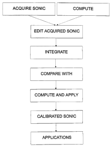
invention;
WO 00/63725 CA 02370665 2001-10-17
PCT/AU00/00343
17
FIG. 5 shows resistivity data, acquired sonic log and a modelled
sonic log from the Waihapa 2 well;
FIG. 6 shows acquired sonic data for the Trulek 1 well;
FIG. 7 shows modelled sonic data for the well of FIG. 6;
FIG. 8 shows acquired sonic data for the Bayu 3 well; and
FIG. 9 shows modelled sonic data for the well of FIG. 8.
List of
abbreviations
and terms
1o a constant used in Archie equation
C compaction constant used in Wyllie equation
C' compaction constant used in Raymer-Hunt-Gardner
equation
a exponential number
F functional operator
F' functional operator
F" functional operator
In interval transit time in microseconds per foot
(inverse of VP)
k constant used in exponent in Korvin compaction
equation
m exponent in Archie equation - associated with
cementation
2 o n exponent in Archie equation - associated with
tortuosity
Res resistivity
RFm" resistivity of formation
Rsna~e resistivity of shale
Rt true resistivity of formation (= RFm~)
V velocity of sound
V; volume of lithologic component
VP velocity of pressure wave (p-wave)
VS velocity of shear wave (s-wave)
VpZ velocity of p-wave at depth z
3 o VsZ velocity of s-wave at depth z
z depth in kilometres
~ T sonic interval transit time
WO 00/63725 CA 02370665 2001-10-17 PCT/AU00/00343
18
TFmn sonic interval transit time of formation
~ To sonic interval transit time at initial depth
~ T~ sonic interval transit time at infinite depth
D T L~ sonic interval transit time at depth z
D Tr"a sonic interval transit time of rock matrix
d T~ sonic interval transit time of fluids in pore spaces
Lame constant related to bulk modulus
g Lame constant (shear modulus)
~,+2p, modulus function (mixed elasticity function)
l0 ~.o Lame bulk constant at initial depth
Lame bulk constant at infinite depth
,u~ Lame shear constant at infinite depth
,uo Lame shear constant at initial depth
porosity
~,son;~ porosity computed from sonic velocity
r bulk density
pb bulk density
~ bulk density at depth z
bulk density at depth z
2 o p~ bulk density at infinite depth
po bulk density at initial depth
Detailed description of the invention.
Acoustic logging devices generate an outgoing acoustic
pulse, part of which, after travelling for some distance through the rocks in
the near vicinity of the borehole, re-enters the borehole and is detected by
a sensor array (Tittman, 1986; Schlumberger, 1989). The elapsed time
WO 00/63725 CA 02370665 2001-10-17 PCT/AU00/00343
19
between transmission and detection is then interpreted in terms of rock
acoustic velocities. While the derived rock properties are influenced by
various factors (including the travel path of the detected wavefront,
borehole geometry, rock framework and fluid properties, fluid invasion in
the near-borehole environment, and pore fluids in the uninvaded rocks)
correct identification of the incoming signal is a fundamental pre-requisite.
Since acoustic data is acquired with a moving logging sonde
(FIG. 1 ), noise arising from contact between the logging sonde and cable,
and the borehole wall is generally present in the logging environment, and
1 o successful acoustic log data acquisition requires differentiation of the
incoming acoustic wave from the noise. This is generally achieved by
amplitude-based detection within a discrete time range. Cutoffs are set
such that the desired incoming wave energy exceeds the background
noise (FIG. 2). Upon wavefront arrival, detection is triggered and the
transit time for the passage of the wave from source to detector is
recorded. The process is repeated many times per second and a
continuous record of transit time versus depth in the borehole results as
the logging sonde travels up the borehole.
Whenever the incoming signal is incorrectly identified, an
2 o erroneous instantaneous transit time results, identified often as
'spiking'
on the transit log. In acoustic logging, this most commonly arises when
noise momentarily overwhelms the incoming signal, resulting in the
detector failing to identify the first arrival, and subsequently responding to
the arrival of a later wavefront (which may have travelled entirely within
the borehole fluid column). Events of this nature may be related to high
noise events, but more frequently result from borehole factors causing
significant attenuation of the acoustic signal (e.g. gas in the borehole
fluid)
or by rock features causing attenuation (e.g. fractures or poor
compaction). In the case of poor compaction, the efficiency of acoustic
3 o transmission is reduced and, if background borehole noise is relatively
constant, noise may overwhelm the desired signal. Such conditions may
persist over significant intervals of hole.
WO 00/63725 CA 02370665 2001-10-17 PCT/AU00/00343
The above equations can be applied in numerous ways to
better quantify the acoustic performance of the sedimentary sequence. A
particular concern in the present invention is the application to sonic log
calibration.
5 With a sonic log of variable quality, the person skilled in the
art can usually recognize intervals where the sonic signal acquisition and
interpretation has resulted in a geologically and geophysically reasonable
outcome, where the sonic signal appears reliable, and intervals where the
converse is true. The main cause of mismatch between integrated sonic
1o times and check-shot interval times is generally systematic signal
misinterpretation (e.g. cycle skipping) over discrete intervals of the hole,
and the objective is to replace the acquired signal across these intervals
with a theoretical signal which honours the above compactive theory.
An approach in the present invention is to use a single shale
lithology as the compactive key, and to use the resistivity data as a
general modifier which corrects for both lithologic and porosity variation
from that expected of shale.
The substitution of theoretical sonic for acquired sonic in
intervals is at present done by skilled interpreters following the steps
2 o shown in FIG. 3. Where the observed sonic departs from the theoretical,
this departure is most commonly due to signal detection misinterpretation
in the sonic logging tool or surface recording equipment. The output of is a
calibrated sonic log that can be used in applications.
The process of the invention begins by computing a suitable
25 synthetic sonic log.
The checking process is a standard well logging technique.
A sound pulse is injected into the near surface, and a travel time to a fixed
depth is precisely measured. This can be repeated at numerous points
down a well, and in this way a precise velocity profile of the rock sequence
3 o can be acquired. This profile should closely match the short-interval data
collected from the well bore (the sonic log) but rarely matches acceptably,
because (at least in part) of noise inherent in the log acquisition process.
WO 00/63725 CA 02370665 2001-10-17 PCT/AU00/00343
21
The checkshot data is considered to be more reliable (much
lower error percentages), and the sonic log data is therefore adjusted
(usually by bulk shift) to force integrated sonic times to match the
observed checkshot times.
In this process, the value in the invention lies in the ability to
substitute a petrophysically reasoned synthetic for the acquired sonic
where the acquired data is in any way suspect, prior to the bulk shift
forcing of the sonic to fit the checkshot data.
The compactive constant k is first determined for each major
to genetic sequence increment. This can be achieved by use of point
density data (from either core or log) to solve the Korvin density function
(equation (1 ) above) for k . Departures from the expected shale
compactive trend usually arise from density reductions due to inclusion of
low density materials (water, organic carbon); these produce erroneously
high estimates of k . If sufficient data are available, a number of
determinations should be made within each major sequence increment,
and the minimum observed value should be chosen for k .
Within a sequence increment and a single geologic domain it
can be expected that variations in k are systematic and mappable. This is
2 o certainly the case on a field scale. If we gather and map data for k , we
should subsequently be able to estimate k for each sequence increment,
removing the need for density data.
Having established values for k, we then proceed to
estimate the modulus function, ~~.+ 2,u~ . If sufficient data are available,
taking observed 0T from intervals of reliable sonic data in shales, we
solve equation (4) above for ~~~+ 2,u~ at a number of points throughout
the sequence, and interpolate between points to give a continuous
estimate of ~~.+ 2,u~ versus depth.
Now having established the distribution of k and ~~. + 2,u~ ,
3 0 solve equation (4) for O Tshale at any depth. Identify intervals of
cleaner
CA 02370665 2001-10-17
WO 00/63725 PCT/AU00/00343
22
shale from the resistivity and any other available logs, and extract values
of shale resistivity at these points. Use the point data to continuously
estimate shale resistivity by linear interpolation. Then apply standard
resistivity to porosity and porosity to 0 T transform techniques to compute
a continuous resistivity difference function, using the shale and general
formation resistivities, to modify the shale velocity and arrive at a mixed
formation velocity, as detailed in equations 10,11 and 12 above.
This is not necessarily the only approach, but there are
powerful practical reasons for using it - robust compactive relationships
to have not been established for non-shale lithologies. Also, in many wells,
particularly pre-1960's wells logged with western technology, and most
wells logged using Russian technology, wireline data may not be sufficient
to permit acceptable lithologic definition using existing techniques.
However, in such wells there is generally sufficient core data to yield shale
bulk density data over sufficient of the sequence to permit the solution of
the Korvin shale density equation for k . There is also usually a basic
resistivity log. If the modulus function is estimated, on regional geologic
and lithologic grounds, a theoretical sonic log can be computed. Then a
synthetic seismogram can be generated, and it can be correlated with
2 0 observed seismic data. Subsequently the modulus function is
reprocessed and iteratively refined to better the estimate of the modulus
function until there is acceptable agreement with the observed seismic.
When considering noise removal and re-computation of
acquired sonic data, by using the above techniques, a continuous
synthetic sonic log can be generated which conforms closely to the
observed sonic over intervals where there is confidence in the acquired
data. We can then systematically and optimally merge the two data sets
to produce an optimized sonic, which can then be calibrated to the check-
shot data in the normal manner. Because we have replaced the observed
3 o data, wherever it is suspect, with data systematically computed on a
mathematically and physically valid model, we can expect the resultant
composite data to be superior to the raw acquired data.
WO 00/63725 CA 02370665 2001-10-17 PCT/AU00/00343
23
We can (and do) systematically check the acceptability of
the output by over-plotting an independent porosity indicator (the neutron
porosity) on top of the optimized sonic plot. Correlation is generally
excellent. This is a better technique than cross-plotting, since depth-
paired data are more readily identified.
Shear Wave Velocity Estimation
~. -E- 2,C1 2 ,ll 2
From hp = and 1~s = - we can establish
p p
Y
that ~s is independent of density, and, it seems, does not vary greatly
1o within each lithology (Gorbachev, Yuri I., 1995 Well logging:
Fundamentals of methods: John Wiley and Sons, 324 p). If we can
establish the lithotype mix, and we have superior hp data, we should
also be able to compute an improved Its (Xu, Shiyu and White, Roy E,
1996, A physical model for shear-wave velocity prediction: Geophysical
Prospecting, v. 44, p. 643-686).
Since the modulus function ~~. + 2,u) is a mixed term, we
cannot extract unique values for the components, and we expect the
components to vary with lithologic variation.
Where hydrocarbons are present, and hole conditions are
2 o acceptable but the sonic log is unreliable, an alternative approach is to
compute porosity from the density log, then transform this porosity into a
theoretical Q r and replace data over the suspect interval. The approach
also cannot be used in coal-bearing sequences. In general, coals show
high resistivities with distinctively slow velocities. Acceptable modelling of
OT in coally sequences requires a mixed-lithology model.
If an alternative and reliable porosity log is available, and
sonic quality is poor (eg due to gas entrained in the drilling mud), a
derived porosity (eg neutron-density) can be substituted in equation (6)
WO 00/63725 CA 02370665 2001-10-17 PCT/AU00/00343
24
above, and solved for ~T . (If gas is present, the neutron porosity is also
affected and cannot be used without prior correction.)
Implementation
There are four elements to implementation of the above
method.
A log data input system. This module takes data in
effectively any form (Log ASCII standard, Log information
standard, Digital log interchange standard, various ASCII
1o forms including non-regularly sampled data), and delivers
regularly sampled, uniformly formatted data to the
mathematical processing engine.
r A mathematical parser and processor. The user is able to
enter algorithms in simple algebraic form, and to process the
15 data into new log forms.
Capacity to build and reference look-up tables. This includes
the ability to control critical parameters over specific depth
ranges, through reference to look-up tables and to apply
various interpolation schemes to these parameters. Thus
2 o the precise form and sequence of algorithms and the inter-
relationship of models is flexible, and can be controlled by
the user. The result is a powerful and flexible interpretative
computational engine.
A data output system. The products of processing are
25 output in the above standard log file formats and can be
displayed within the software or output to files for use in
other display or application modules.
The technique can be used to improve the quality of
acquired compression wave sonic data by selective replacement of
3 o intervals of poor quality or absent data. Where there is reliable sonic
log
data in the overlying and underlying rocks, Korvin's compaction constant
k can be determined from bulk density data. The slowness equation can
W~ 00/63725 CA 02370665 2001-10-17
PCT/AU00/00343
then be solved for the mixed elasticity function. These data are then used
to generate the expected shale velocity through the interval of interest,
and resistivity data are used to generate the desired composite
compression DT. The generated data then replaced the poor quality or
5 absent data over the interval of interest.
In Waihapa 2 (onshore Taranaki Basin, New Zealand),
between 9902 feet and 10017 feet, both regular and long spaced sonic
signals are meaningless (FIG. 5). Other logs across the interval are
considered reliable, and the hole is near-gauge. Since the indicated
1o porosities in the surrounding section are relatively low, the Wyllie time-
average transform is used to convert resistivity-based porosity into a
slowness component, which is then added to the Korvin-based shale
slowness, to arrive at a composite slowness for the missing section. FIG.
5 shows the computed data plotted versus other data. There is good
15 agreement between the acquired 0T and that computed, over the section
above and below the interval of interest.
In Trulek 1 (offshore, Timor Sea, western Undan-Bayu field,
Australia), long intervals of the acquired sonic log data are suspect (FIG.
6). Using the combination of Korvin shale compaction and wireline log
2 0 resistivity -porosity transforms, it is possible to generate a computer
slowness curve which shows good agreement (FIG. 7) with the acquired
data over long intervals where the acquired sonic is considered reliable.
The comparison suggests we can have reasonable confidence in the
computer slowness where comparative data is not available.
25 In Bayu 3 (Undan-Bayu field, Timor Sea, Australia) there is a
long interval over which no openhole log data is acquired as a result of
difficult drilling conditions (FIG. 8). Using measurement-while-drilling
data, it is possible to generate a computed slowness curve to infill the
interval where sonic data is absent (FIG. 9).
OTHER APPLICATIONS. A sonic log model which is both theoretically
valid, and of demonstrated practicality, has very wide potential application
WO 00/63725 CA 02370665 2001-10-17 PCT/AU00/00343
26
in the geological and geophysical sciences. The algorithm describes
compaction, and can be inverted to yield both erosional losses and de-
compacted thickness at prior times in the evolution of a basin sequence.
This has potentially great significance in modelling hydrocarbon systems
and migration pathways associated with peak migration episodes for these
systems.
Where shale pore pressures are known (eg from drilling
measurement), shale departure from the expected compactive trend-line
to lesser density can be interpreted quantitatively in terms of organic
1o carbon content. We are presently gathering chemical analytical data to
permit systematic interpretation of sonic data in these terms.
The constant k should be systematically mappable across
basins, for each major genetically related sediment package. Once so
mapped, such data should considerably refine present time-depth
conversion procedures based on seismic. When even scattered data are
present, better regional seismic interpretations should be possible.
The relationship between rock sequence age, thermal
history, and maturation is of fundamental importance to modelling of
hydrocarbon generation and primary migration. We expect an empirical
2 o correlation, if not a causative analytical link, between shale density and
0 T , and observed levels of organic metamorphism.
Systematic estimation and mapping of the modulus function
~~, + 2,u~ should significantly improve our ability to interpret seismic data.
A new model describing systematic changes in shale density
and acoustic performance with depth of burial has been established. This
model is based on physical and mathematical analysis, is not empirical,
has few constraints, and yields results which appear superior to those of
previously published models. When applied to field acoustic log data, this
model gives significant improvements in log data quality. Editorial
3 o improvement of the sonic log quality, conducted in this manner, yields a
log which is no worse than the original, and may be vastly superior for
W~ 00/63725 CA 02370665 2001-10-17
PCT/AU00/00343
27
purposes of seismic study. The edited log should then be subject to
normal calibration before use in seismic studies.
The model has potential for diverse and very significant
applications in basins analyses and study of hydrocarbon systems.
The underlying mathematical-physical model has far-
reaching implications for study of sedimentary sequences, hydrocarbons
systems and whole basin analyses.
Sequence compaction and acoustic wave propagation
theory, supported by sonic and other log data from several thousand wells
1o in a number of Australasian sedimentary basins, have led to the
development of an alternative method of editorial enhancement of sonic
log data. The technique and derivative concepts have potentially far-
reaching applications in basin study and basin analysis.
Areas of application include, but are not limited to:
25 1. Computation of theoretical sonic data to replace intervals
where acquired data is either noisy or absent. This leads to
improved sonic log quality, yielding improved well to regional
seismic ties.
2. Improved interpretation of seismic data in terms of seismic
2 o time to depth conversion.
3. Theoretical de-compaction of sequences, allowing improved
reconstruction of basin geometry at prior times in the earth's
history.
4. Interpretation of improved sonic data in terms of rock
25 reservoir properties, yielding better understanding of
reservoir performance, with improved exploitation economies
and better total recoveries from known fields.
All the above are each quite large areas of commercial
activity.
3 o Throughout the specification the aim has been to describe
the preferred embodiments of the invention without limiting the invention
to any one embodiment or specific collection of features.