Note: Descriptions are shown in the official language in which they were submitted.
CA 02370772 2002-O1-24
Descriution
FIELD OF THE INVENTION
Despite the success of relay feedback system in autotune identification, it is
well known that a relay
based identification can lead to significant errors in the ultimate gain and
ultimate frequency. The
errors come from the linear approximation (describing function method) to a
nonlinear element. The
square type of output from the relay is approximated with the principal
harmonic from the Fourier
series (Derek P. Atherton, "Nonlinear Control Engineering", Van Nostrand
Reinhod: Nev York,
1982) and the ultimate gain is estimated accordingly. Several attempts were
proposed to overcome
this inaccuracy but didn't overcome the main source of inaccuracy - linear
approximation of the
relay element due to the use of describing function method model. The present
invention
completely eliminates this source of inaccuracy - on account of application of
a precise model of
the oscillatory process - via the use of the locus of a perturbed relay system
(LPRS) method (Igor
Boiko, "Input-output analysis of limit cycling relay feedback control
systems," Proc. of 1999
American Control Conference, San Diego, USA, Omnipress, 1999, pp.542-546; Igor
Boiko;
"Application of the locus of a perturbed relay system to sliding mode relay
control design," Proc. of
2000 IEEE International Conference on Control Applications, Anchorage, AK,
USA, 2000, pp.
542-547; Igor Boiko, "Frequency Domain Approach to Analysis of Chattering and
Disturbance
Rejection in Sliding Mode Control," Proc. of World Multiconference on
Systemics, Cybernetics and
Informatics, Orlando, Florida, USA, Vol. XV, Part II, pp. 299-303) instead of
describing function
method. The present invention defines a method and an apparatus for bringing
the system
(comprising the process, nonlinear element and external source of constant set
point signal) into
asymmetric oscillations mode (further referred to as asymmetric oscillatory
experiment) for
determining (measuring) quantities essential for the tuning of the controller.
The invention includes
all variations and combinations (P, PI, PD, PID, etc.) of the control types of
PID controller but not
limited to those types of controllers.
BACKGROUND OF THE INVENTION
Autotuning of PID controllers based on relay feedback tests received a lot of
attention recently (W.
L. Luyben, "Derivation of Transfer Functions for Highly Nonlinear Distillation
Columns", Ind.
Erg. Chem. Res. 26, 1987, pp.2490-2495; Tore Hagglund, Karl J. Astrom,
"Industrial Adaptive
CA 02370772 2002-O1-24
2
Controllers Based on Frequency Response Techniques", Automatica 27, 1991,
pp.599-609). It
identifies the important dynamic information, ultimate gain and ultimate
frequency, in a
straightforward manner. The success of this type of autotuners lies on the
fact that it is simple and
reliable. The appealing feature of the relay feedback autotuning has lead to a
number of commercial
autotuners (Tore Hagglund, Karl J. Astrom, "Industrial Adaptive Controllers
Based on Frequency
Response Techniques", Automatica 27, 1991, pp.599-609) and industrial
applications (H. S.
Papastathopoulou, W. L. Luyben, "Tuning Controllers on Distillation Columns
with the Distillate-
Bottoms Structure", Ind. Eng. Chem. Res. 29, 1990, pp.1859-1868).
Luyben (W. L. Luyben, "Derivation of Transfer Functions for Highly Nonlinear
Distillation
Columns", Ind. Eng. Chem. Res. 26, 1987, pp.2490-2495) pioneers the use of
relay feedback tests
for system identification. The ultimate gain and ultimate frequency from the
relay feedback test are
used to fit a typical transfer function (e.g., first-, second- or third order
plus time delay system).
This identification procedure is called the ATV method. It was applied
successfully to highly
nonlinear process, e.g., high purity distillation column. Despite the apparent
success of autotune
identification, it can lead to signification errors in the ultimate gain and
ultimate frequency
approximation (e.g., 5-20% error in R. C. Chiang, S. H. Shen, C. C. Yu,
"Derivation of Transfer
Function from Relay Feedback Systems", Ind. Eng Chem. Res. 31, 1992, pp.855-
860) for typical
transfer functions in process control system.
The present invention completely eliminates the source of inaccuracy that
comes from the linear
approximation to the nonlinear element - via the use of the LPRS method
instead of describing
function method. The LPRS describes a relay system just like the transfer
function describes a
linear system. The present invention defines a method and an apparatus for
bringing the system into
asymmetric oscillations mode for measuring quantities essential for tuning a
controller. More
accurate description of the oscillations in the relay system allows for more
precise identification of
the parameters of the process model and a better quality of tuning a
controller.
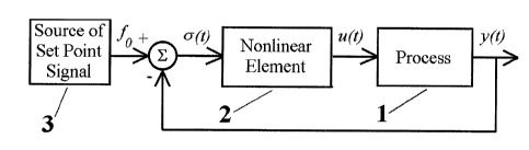
BRIEF DESCRIPTION OF THE DRAWINGS
FIG. 1. The system that comprises the nonlinear element, the process, and the
source of the set point
signal.
CA 02370772 2002-O1-24
3
FIGS. 2A and 2B. Input-output relationship for symmetric hysteresis relay and
asymmetric
hysteresis relay.
FIG: 3. Block diagram of a relay feedback system.
FiG. 4. LPRS and determination of the frequency of oscillations.
FIG. 5. Block diagram of the controller and the process.
FIG. 6. Block diagram of the SIMULINK° model of the autotuning
system.
DETAILED DESCRIPTION OF THE PREFERRED EMBODIMENT
Refernng to the drawings, a description will be given of an embodiment of a
controller autotuning
method according to the present invention.
The PID-control stands for proportional, integrating and derivative control.
It is very common for
controlling industrial processes. PID-controllers are manufactured by various
manufacturers in
large quantities. Usually the controllers are based on microprocessors and
proportional, integrating
and derivative functions are normally implemented within a software.
Nevertheless, the principal
structure of a conventional PID-controller is retained and without loss of
generality it is possible to
consider a PID-controller as a parallel connection of three channels:
proportional with gain Kp,
integrating with gain K; and derivative with gain Kd. As a result, transfer
function of the PID-
controller is:
Wpid~SJ- Kp + KT ~S -~ Kd S
Choice of gains Kp, KI and Kd values is a subject of tuning if the controller
is implemented as a PID-
controller. There are established methods of tuning a PID-controller in
dependence on the
parameters of the process, for example Ziegler-Nichols's method of manual
tuning, Hagglund-
Astrom's relay feedback autotuning method. There are also a number of other
methods of manual
and automatic tuning. All those methods can be divided into parametric and non-
parametric.
CA 02370772 2002-O1-24
Parametric methods are based on a certain dynamic model of the process with
unknown parameters.
The process undergoes a test or a number of tests aimed at the process model
parameters
identification. Once the process model parameters are identified, the
controller is tuned in
accordance with known from the automatic control theory rules - to provide
stability and required
performance to the closed-loop system (comprising the process, the controller,
the comparison
device, and the feedback). Non-parametric methods are based on the tests on
the process, which are
aimed at the measurement of some general characteristics of the process, for
example ultimate gain
and ultimate frequency at both Ziegler-Nichols's method of manual tuning and
Hagglund-Astrom's
relay feedback autotuning method.
Generally, parametric methods can provide a better tuning quality (due to
possibility of the use of
more precise model of the process) but require more complex tests on the
process. Therefore, there
is a need for comparatively simple yet precise method of tuning (manual and
automatic), which can
be embedded into software of local controllers or distributed control system
(DCS) or be
implemented as a software for a personal computer used by an engineer who is
supposed to tune the
controllers.
Usually, methods of tuning that utilize Hagglund-Astrom's relay feedback test
for estimating the
parameters of oscillations are based on describing function method (Derek P.
Atherton, "Nonlinear
Control Engineering", Van Nostrand Reinhod: New York, 1982). The use of this
method is limited
to harmonic oscillations in the system, which is normally not the case.
The present invention is based on the model of oscillations provided by the
LPRS method (Igor
Boiko, "Input-output analysis of limit cycling relay feedback control
systems," Proc. of 1999
American Control Conference, San Diego, USA, Omnipress, 1999, pp.542-546; Igor
Boiko,
"Application of the locus of a perturbed relay system to sliding mode relay
control design," Proc. of
2000 IEEE International Conference on Control Applications, Anchorage, AK,
USA, 2000, pp.
542-547; Igor Boiko, "Frequency Domain Approach to Analysis of Chattering and
Disturbance
Rejection in Sliding Mode Control," Proc. of World Multiconfe.rence on
Systemics, Cybernetics and
Informatics, Orlando, Florida, USA, Vol. ~V, Part II, pp. 299-303), which
doesn't use the above
limiting hypothesis. The present invention provides a relatively simple
parametric method of
controller tuning. The method uses a modified Hagglund-Astrom's relay feedback
test as means to
CA 02370772 2002-O1-24 -
identify parameters of a process model: A process can be modeled by a transfer
function with a
dead time (time delay) or without it or have a matrix state space description.
According to the present invention, a method is provided where the process has
a transfer function
Wp(s) or a matrix state space description and the system (Fig. 1 ) - via
introduction a nonlinear
element 2 in series with the process 1 and applying a set point signal 3 to
the closed-loop system - is
brought in asymmetric self excited oscillations mode for measuring the
frequency of the
oscillations, average over the period value of the process output signal and
average over the period
control signal whereupon the controller is tuned in dependence on the
measurements obtained. An
element having a non-linear (relay) characteristic (Fig. 2A or 2B) is
introduced into the system in
series with the process and set point signal is applied to excite asymmetric
self excited oscillations
in the system. If the nonlinear element has an asymmetric relay characteristic
the system should be
transformed into an equivalent relay system with a symmetric relay
characteristic - with the use of
known from the automatic control theory techniques.
It is proved (Igor Boiko, "Input-output analysis of limit cycling relay
feedback control systems,"
Proc. of 1999 American Control Conference, San Diego, USA, Omnipress, 1999,
pp.542-546; Igor
Boiko, "Frequency Domain Approach to Analysis of Chattering and Disturbance
Rejection in
Sliding Mode Control," Proc. of World Multiconference on Systemics,
Cybernetics and Informatics,
Orlando, Florida, USA, Vol. XV, Part II, pp. 299-303) that asymmetric self
excited oscillations in
the relay feedback system (Fig. 3) comprising the process transfer function 1,
the relay 2, the set
point signal 3, the feedback 4, and the comparison device 5 can be described
by the LPRS. The
LPRS is a characteristic of a relay feedback system that has the following
definition:
J(u~) _ -0.5 lim 6" + j -'~, lim y(t)~,_o (1)
~o-~~ u" 4c t~-~
where f~ is the set point, 6o and uo are constant terms of error signal 6(t)
and control u(t)
respectively, c is the amplitude of the relay, ~ is the frequency of the
oscillations, which can be
varied by means of varying the hysteresis b of the relay.
The LPRS is related with a transfer function of the linear part of a relay
feedback system, and for a
given transfer function W(s) of the linear part of a relay feedback system the
LPRS J(~) can be
CA 02370772 2002-O1-24
6
calculated via the use of one of the following formulas and techniques (Igor
Boiko, "Input-output
analysis of limit cycling relay feedback control systems," Proc. of 1999
American Control
Conference, San Diego, USA, Omnipress, 1999, pp.542-546; Igor Boiko,
"Application of the locus
of a perturbed relay system to sliding mode relay control design," Proc. of
2000 IEEE International
Conference on Control Applications, Anchorage, AK, USA, 2000, pp. 542-547;
Igor Boiko,
"Frequency Domain Approach to Analysis of Chattering and Disturbance Rejection
in Sliding
Mode Control," Proc. of World Multiconference on Systemics, Cybernetics and
Informatics,
Orlando, Florida, USA, Vol. XV, Part II, pp. 299-303):
a) The LPRS can be calculated as a series of transfer function values at
multiple frequencies -
according to the formula:
J(a~) _ ~k"'(-1)~'+'ReW(kw)+ j~ 1 ImW~(2k-1)tvJ (2)
h=, ~-! 2k -1
where W(s) is the transfer function of the linear part of the system (of the
process in this case), m=D
for type zero (non-integrating process) and m=1 for non-zero type servo system
(integrating
process). For realization of this technique, summation should be done from k=1
to k=MI and M~
where MI and MZ are sufficiently large numbers for the finite series being a
good approximation of
the infinite one.
b) The LPRS can be calculated with the use of the following technique.
Firstly, transfer function is
represented as a sum of m transfer functions of 1 S' and 2"d order elements
(expanded into partial
fractions):
W(s)=W~(s) + W2(s) + W3(s) + ... + Wm(s)
Secondly, for each transfer function, respective LPRSs (the partial LPRSs) are
calculated with the
use of formulas of Table 1.
CA 02370772 2002-O1-24
Tahle 1. Formulas of LPRS J(CV)
Transfer function LPRS J(w)
W(s)
Kls 0 j~Kl(8~)
Kl(Ts+1) O.SK(1-acosech tx);j0.25~rKth(txl2), tx-~(T~)
Kl(( T~s+I)( T2s+1)JO. SKjl -Til(T~-TZ) a~ cosech al- T2/( Tz-
T~) gel cosech tx~)J
j0.25~cK1(TI-T~ jT, th(cel2) - Ti th(a2/2)J,
a,~(T w),
txa~l(Ta~)
K/(s~+2~s+1) 0.5 Kj(1-(B+yC)l(sinZ/3+sh2cx)J
j0.25~K(shca ysin~3) l (cha'+-cos~
a~c~l~, ia~t(1-~)liz/~ ~~/~~
B~cos,(3sha+psin~icht~ C=asin,Ochc~-J3cosjishtx
K sl(s2+2~s+1) 0.5 K j~ (B+yC) - ~lw cos/3shtxJ l(sinZj3+sh~a)J
j0.25 K ~'(I-~)-~~~ sin,l3/ (chcx+cos,~
a-~~1~, /3-~c(I-~)'i2/~, . y-~~~
B=~ecos~l3sha+,(isin,l3ch~ C=c~sin/3cha-/3cos~3sha,
Ksl(s+1) 0.5 K ja(sha+ tech a)lsh?a -~j0.25~ca1(I
+ cha)J, a-~rl~
Kslj(Tls+1)(TZS+l)J D.5 Kl(T2-T,) j as cosech ct2-al cosech ~x~J
j0.25 K Jrl(T2-T~) j th(cell2) - th(azl2)J,
al=~l(T ~), a2 ~cl(T2~)
Thirdly, the LPRS is calculated as a sum of all partial LPRSs:
J(w)°J~(~) + JZ(~) + J3(~) + ... + Jm(~)
c) For matrix state space description, the LPRS for type 0 servo systems is
calculated with the use
of formula (3):
CA 02370772 2002-O1-24
J(to) _ -O. SC(A-' + 2~ (1- a 1°' A)-'e°'AJB
w (3)
+j 4C(1+e~A)-'(1-e~A)A-'B
where A, B and C are matrices of the following state space description of a
relay system:
x=Ax+Bu
y=Cx
+IifQ=fo-Y>b,h>0
u=
-lif 6--fo-y<-b,d~<0
where A is an nxn matrix, B is an nxl matrix, C is an 1 xn matrix, f0 is the
set point, c: is the error
signal, 2b is the hysteresis of the relay function, x is the state vector, y
is the process output, a is the
control, n is the order of the system;
or the LPRS for type 1 (integrating process) servo systems is calculated with
the use of formula (4):
J(~) = 0.25CA-'((I-DZ)-'~Dz
-(I+4~ A)D+D3 -I]+D-IjB+
a'
+ j'~ CA-'~ ~ +A-'C(1-DZ)-'
8 ~
~(3DZ -3D-Dj +I)-D+IJ)B,
~A
where D = a ~ , A, B and C are matrices of the following state space
description of a relay system:
X=Ax+Bu
.Y=Cx-fo
!~+lif ~=-y>b,~>D
u-
-lifer=-y<-b,d~<0
where A is an (n-1)x(n-1) matrix, B is an (n-I)xl matrix, C is an 1 x(n-I)
matrix, n is the order of
the system.
CA 02370772 2002-O1-24
9
Any of the three techniques presented above can be used for the LPRS
calculation. If the LPRS is
calculated (Fig. 4) the frequency of oscillations .S2 and the equivalent gain
of the relay k" can be
easily determined. In a relay feedback system, the following equalities are
true (directly follow
from the LPRS definition above; detailed consideration is given in the paper:
I. Boiko, "Input-
output analysis of limit cycling relay feedback control systems," Proc. of
1999 American Control
Conference, San Diego, USA, Omnipress, 1999, pp.542-546):
Im J(Sa) _ - ~b- , (5)
__ 1
k" 2Re J(SZ) (6)
The frequency of oscillations S2 corresponds to the point of intersection of
the LPRS 1 and the line
2 parallel to the real axis that lies below it at the distance of ~$/(4c).
Therefore, by measuring
frequency of oscillations ,f~, average over the period process output yo and
average over the period
control signal uo we can calculate average over the period value of the error
signal:6o fo yo, ~e
equivalent gain of the relay k"= uola-o (although this is not an exact value
the experiments prove that
it is a very good approximation even if uo and ~o are not small; the smaller
uo and ~o the more
precise value of k,~ we obtain), the static gain of the process K= y~luo, and
identify one point of the
LPRS - at frequency S2.
J(.~) =-os (fn yo)luo - j ~bl(4c)
If the model,of the process contains only 2 unknown parameters (beside static
gain 1~, those two
parameters can be found from complex equation (7), which corresponds to
finding a point of the
LPRS at frequency X52.
If the process model contains more than three unknown parameters, two or more
asymmetric
oscillatory experiments - each with different hysteresis b of the relay
element- should be carried
out. As a result, each experiment provides one point of the LPR.S, and N
experiments provide N
CA 02370772 2002-O1-24
points of the LPRS on the complex plane enabling up to 2N unknown parameters
(beside static gain
K) to be determined.
One particular process model is worth an individual consideration. The first
reason is that it is a
good approximation of many processes. The second reason is - this process
model allows for a
simple semi-analytical solution. The process transfer function Wp(s) is sought
to be of 1 S' order with
a dead time:
Wp(s)=K exp( zs) l (Ts+1) (8)
The LPRS for this transfer function is given by:
_r' Y
J(co) = K (1- a eYCOSech a) + j'-' K ( 2e .-a . _ I) (9)
2 4 I+e-a
where K is a static gain, T is a time constant, zis the dead time, c~~tl~T,
y=tlT
With the measured values ,Sl, y~ and u~ and known f~, b and c, parameters K, T
and zof the
approximating transfer function are calculated as per the following algorithm:
(a) at first the static gain K is calculated as:
K-Yo
a (10)
(b) then the following equation is solved for ~x
Ya=1.._-~~. (11)
.fo a '
(c) after that time constant T is calculated as:
T aSl ' (12)
(d) and finally dead time 2-is calculated as:
i = T Ink ~ (ea + I)j (13)
The most time consuming part of the above algorithm is solving equation (11).
This is a nonlinear
algebraic equation and all known methods can be applied for its solution.
CA 02370772 2002-O1-24
t1
With the parameters K, T and zof the approximating transfer function
identified, PI controller can
be easily designed. The following tuning algorithm/values are proposed.
Proportional gain Kp and
integrator gain Ki in PI control are calculated as follows. For desired
overshoot being a constraint,
proportional gain Kp and integrator gain K; are sought as a solution of the
parameter optimization
(minimization) problem with settling time being an objective function. This
allows to obtain a
minimal settling time at the step response as well as appropriate stability
margins at any law of set
point change.
A simplified solution of this problem is proposed by this invention too. It is
proposed that quasi-
optimal settings.are used instead of optimal settings. Those are obtained as a
solution of the above
formulated optimization problem and respective approximation. Gains Kp and K,
as functions of
desired overshoot are approximated. At first normalized values of KP and KI
denoted as K°n and K°;
should be calculated as follows:
For overshoot 20% integrator gain is calculated as K°; =1.60z/l;
(14)
for overshoot 10% K°;=1.80a/I'; (15)
for overshoot 5% K°1=1.952Yf. (16)
Normalized proportional gain K°p is to be taken from Table 2 with in-
between values determined
via interpolation.
Table 2. Quasi-optimal settings of PI controller (proportional gain
K°p)
Overshootz/T z~f z~!' z/f zll Z/I' zlT 2/I' z/f zlT z/f
[%] =0.1 =0.2 =0.3 =0.4 =0.5 =0.6 =0.7 =0.8 =0.9 =1.0 =1.5
20 K"p 3.7022.5642.0071.6831.4731.3291.2251.1461.0860.915
=7.177
Kp 3.0582.1201.6731.4191.2581.1481.0681.0080.9630.833
=5.957
5 K' 2.6241.8231.4831.2941.1701.0821.0140.9640.9240.808
p
=5.203
CA 02370772 2002-O1-24
12
Finally, Kp and K; are calculated as Kp = K°,, /K and K; K°;/K
where K is the static gain of the
process determined by (10). Formulas (14)-(16) and Table 2 give quasi-optimal
normalized values
of PI controller settings for a desired overshoot.
In some cases an external unknown constant or slowly changing disturbance
(static load) is applied
to the process. In that case the static gain of the process is calculated on
the basis of two
asymmetric oscillatory experiments - each with different average over the
period control signal - as
a quotient of the increment of average over the period process output signal
and increment of
average over the period control signal.
Sometimes the process has a nonlinear character. In this case multiple
asymmetric oscillatory
experiments are to be performed with decreasing values of the output amplitude
of the relay - with
the purpose to obtain a better local approximation of the process. Parameters
of the process transfer
function corresponding to a local linear approximation of the process are
found as a solution of
equations (7), (10) where the process model is expressed as a formula of the
LPRS and contains the
parameters to be identified.
More complex models of the process can also be used. 1.f the process model has
more than 3
unknown parameters, multiple asymmetric oscillatory experiments are performed
with different
values of hysteresis bk (k=1,2...) of the relay - with the purpose to identify
several points of the
LPRS:
ReJ(.fl~= _ ~ .~ou yox (I~)
o~
Im J(.s2kj=-~kl(4c) (18)
where S2~ , yap, uok are .fl, yo, uo corresponding to k th asymmetric
oscillatory experiment.
Each experiment allows for identification of one point of the LPRS and
consequently of two
parameters (beside the static gain). As a result, 2N+1 unknown parameters can
be identified from N
asymmetric oscillatory experiments via solution of 2N+1 nonlinear algebraic
equations (10), (17),
CA 02370772 2002-O1-24
13
(18) with the unknown parameters expressed through a formula of the LPRS.
Therefore, the
number of asymmetric oscillatory experiments can be planned accordingly,
depending on the
number of unknown parameters.
Alternatively, parameters of process transfer function are to be found as
least squares criterion (or
with the use of another criterion) approximation of the LPRS - if the number
of unknown
parameters of the process is less than 2N+1 (where N is the number of
asymmetric oscillatory
experiments). In other words, the LPRS represented via certain process model
parameters is fitted
to the LPRS points obtained through the asymmetric oscillatory experiments. .
Eventually, the designed self tuning PID (or another type) controller is
supposed to be realized as a
processor based (micro-computer or controller) device and all above formulas,
the nonlinear
element, the tuning rules are realized as computer programs with the use of
applicable programming
languages. The preferred embodiment of the controller is depicted in Fig. 5.
The controller 1 has
two AlD converters 2 and 3 on its input for the process output and set point
signals respectively
(alternatively it may have only one A/D converter for the process output
signal, and the set point
may be realized within the controller so$ware), a processor (CPU) 4, a read-
only memory (ROM) 5
for program storage, a random access memory (RAM) 6 for buffering the data, an
addressldatalcontrol bus 7 for data transfer to/from the processor, and an D/A
converter 8 that
converts digital control signal generated by the controller into analog
format. The analog control
signal is applied to the process 9 (to a control valve, etc.). All elements of
the controller interact
with each other in a known manner. Some elements of the controller listed
above (for example A/D
and D/A converters) may be missing as well as the controller m.ay also contain
elements other than
listed above - depending on specific requirements and features of the control
system.
EXAMPLE
The following example illustrates an application of the method as well as is
realized with the
software, which actually implements the described algorithm and formulas. ,
Let the process be described by the following transfer function, which is
considered unknown to the
autotuner and is different from the process model used by the autotuner:
CA 02370772 2002-O1-24
14
W(s)=O.Sexp(0.6s)l(0.8s2+2.4s+1)
The objective is to design a PI controller for this process with the use of
first order plus dead time
transfer function as an approximation of the process dynamics.
Simulations of the asymmetric oscillatory experiment and of the tuned system
are done with the use
of software SIMULINK~ (of MathWorks). The block diagram is depicted in Fig. 6.
Blocks
Transport Delay l and Transfer Fcn 2 realize process model. The control is
switched from the
relay control (blocks Sign 3 and Gain 4) for the asymmetric oscillatory
experiment to PI control
(blocks Gainl 5, Integrator 6, Gain2 7, Suml 8) by the Switch 9 depending on
the value of block
Constant 10 ( 1 for the relay control and -1 for the PI control). Error signal
and control signal are
saved as data files named Error (block To Workspace 11) and Control (block To
Workspace) 12)
respectively. They are processed for calculation of the average output value,
average control value
and the frequency of oscillations. Process output and control signal can be
monitored on Scope 13
and Scope) 14 respectively. Set point is realized as an input step function
(block Step 15). Error
signal is realized as difference between the set point signal and process
output by block Sum 16.
Let us use first order plus dead time transfer function for the
identification:
Wp(s) =Kexp( zs)l(Ts + 1)
Let us choose set point value (final value of the step function) f~=0. l,
amplitude of the relay c=1
and hysteresis b=0 and run the asymmetric oscillatory experiment. The
following values of the
oscillatory process are measured:
Frequency of oscillations S2=1.903,
Average value of the process output y~=0.0734,
Average value of the control signal u0=0.1455.
The following three equations should be solved for K, T, and Z.
1 fo -yo
Re J(S~K, T, 2)= _ 2 uo ,
CA 02370772 2002-O1-24
Im J(Sl,K,T, z)=-~bl(4c),
K Yo l uo
where the formula of J(~) is given by (9).
According to the algorithm described above, the following values of the
process parameters are
obtained from the above three equations:
K=0.5050, T=2.5285, 2=0.9573.
Calculate the settings of the PI controller for the desired overshoot 10% and
the above values of the
identified parameters. As per formula (15) and Table 2 (with the use of linear
interpolation),
K;=1.349 and Kp=3.503. Simulation of the system with the designed PI
controller produces a step
response with overshoot of about 12.5% and settling time about 2.05s (at level
~12.5%). Error
between the desired overshoot (10%) and the actual overshoot (12.5%) is mainly
due to the use of
an approximate model of the process but is also due to the use of the quasi-
optimal values of the PI
controller settings instead of the optimal values.