Note: Descriptions are shown in the official language in which they were submitted.
CA 02452215 2003-12-24
WO 03/023452 PCT/GB02/04121
DETECTION OF SUBSURFACE RESISTIVITY CONTRASTS
WITH APPLICATION TO LOCATION OF FLUIDS
Technical Field
This invention relates to a method of mapping subsurface resistivity
contrasts. The method
enables the detection and location of subsurface resistivity contrasts, which,
in turn, enables
the discrimination between, for example, water (brine or fresh water), which
is conductive,
and hydrocarbons (gas or oil), which are resistive.
Porous rocks are saturated with fluids. The fluids may be water (brine or
fresh water), or
hydrocarbons (gas or oil). The resistivity of rocks saturated with
hydrocarbons is often
orders of magnitude greater than the resistivity of rocks saturated with water
(e.g. 1,000 S2 m
for hydrocarbons vs. 1 S2 m for water). That is, hydrocarbons are resistive
and water is
conductive. If a potentially hydrocarbon-bearing subsurface geological
structure has been
discovered, for instance by seismic exploration, it is important to know,
before drilling,
whether it is resistive (hydrocarbons), or conductive (water). Electromagnetic
methods have
the potential to make this discrimination and thereby reduce the risk of
drilling dry holes.
However, despite decades of research and development in this field, there is
still no routine
procedure for acquiring and processing electromagnetic data to make this
distinction and to
recover subsurface maps representing resistivity variations.
Backsround Art
The known prior art can be summarised in the following papers which are
discussed more
fully below.
[1] McNeill, J.D., 1999, Principles and application of time domain
electromagnetic
techniques for resistivity sounding, Technical Note TN-27, Geonics Ltd.
[2] Zhdanov, M.S., and Keller, G.V., 1994, The geoelectrical methods in
geophysical
exploration: Elsevier
[3] Eaton, P.A., and Hohmann, G.W., 1989, A rapid inversion technique for
transient
electromagnetic soundings: Physics of the Earth and Planetary Interiors, 53,
384-404.
[4] Strack. K.-M, 1992, Exploration with deep transient electromagnetics:
Elsevier
[5] Christensen, N.B., 2002, A generic 1-D imaging method for transient
electromagnetic
data: Geophysics, 67, 438-447.
[6] Strack, K.-M., 1985, Das Transient-Elektromagnetische
Tiefensondierungsverfahren
angewandt auf die Kohlenwasserstoff and Geothermie-Exploration, in: Ebel, A.,
CA 02452215 2003-12-24
WO 03/023452 PCT/GB02/04121
2
Neubauer, F.M., Raschke, E., and Speth, P., (Hrsg.), Mitteilungen aus dem
Institut fiir Geophysik and Meteorologie der LTniversitat zu Koln 42.
[7] Cheesman, S.J., Edwards, R.N., and Law, L.K., 1990, A test of a short-base-
line sea-
floor transient electromagnetic system: Geophysical Journal International,
103, 2, 431-
43 7.
[8] Cairns,G.W., Evans,R.L. & Edwards,R.N., 1996. A time domain
electromagnetic
survey of the TAG hydrothermal mound, Geophys.Res.Lett.,23,3455-3458.
[9] Cheesman, S. J., Edwards, R. N., and Ghave, A. D., 1987, On the theory of
sea-floor
conductivity mapping using transient electromagnetic systems: Geophysics, 52,
204-
217.
[10] Yu, L., Evans, R.L., and Edwards, R.N., 1997, Transient electromagnetic
responses in
seafloor with triaxial anisotropy: Geophysical Journal International, 129, 300-
306.
[11] Eidesmo, T., Ellingsrud, S., MacGregor, L.M., and Constable, S., Sinha,
M.C.,
Johansen, S., Kong, F.N., and Westerdahl, H., 2002, Sea Bed Logging (SBL), a
new
method for remote and direct identification of hydrocarbon filled layers in
deepwater
areas: First Break, 20, 144-152.
[12] MacGregor, L.M., Constable, S., and Sinha, M.C., 1998, The RAMESSES
experiment-
III. Controlled-source electromagnetic sounding of the Reykjanes Ridge at 57
45N:
Geophysical Journal International, 135, 773-789.
[13] MacGregor, L.M., Sinha, M.C., and Constable, S., 2001, Electrical
resistivity structure
of the Valu Fa Ridge, Lau basin, from marine controlled source electromagnetic
sounding Geophys. J. Int., 146, 217-236.
[14] Ziolkowski, A., Hobbs, B.A., Andrieux, P., Riiter, H., Neubauer, F., and
Hordt, A.,
1998. Delineation and monitoring of reservoirs using seismic and
electromagnetic
methods: Project Number OG10305/92/NL-UK, Final Technical Report to European
Commission, May 1998.
[15] Wright, D.A., Ziolkowski, A., and Hobbs, B.A., 2001, Hydrocarbon
detection with a
multi-channel transient electromagnetic survey: Expanded Abstracts 71st SEG
Meeting, 9-14 September, San Antonio, p 1435-1438.
Conventionally time domain electromagnetic investigations use a transmitter
and a receiver,
or a transmitter and a number of receivers. The transmitter may be a grounded
dipole
(electric source) or a wire loop or mufti-loop (magnetic source) and the
receiver or receivers
may be grounded dipoles (electric receivers - recording potential differences
or electric
fields) or wire loops or mufti-loops or magnetometers (magnetic receivers -
recording
magnetic fields and/or time derivatives of magnetic fields). The transmitted
signal is usually
formed by a step change in current in either an electric source or in a
magnetic source.
Known prior developments include (1) a methodology frequently termed TDEM and
often
taken to imply a magnetic source and a magnetic receiver, (2) the Long Offset
Time-Domain
CA 02452215 2003-12-24
WO 03/023452 PCT/GB02/04121
3
Electromagnetic Method (LOTEM) developed for land surveys, (3) time domain
electromagnetics in the marine environment (University of Toronto/Scripps
Institution of
Oceanography), (4) Sea Bed Logging (SBL) using single frequency
electromagnetic
measurements in the marine environment (Scripps Institution/ Southampton
Oceanography
Centre/ Electromagnetic Geophysical Services Ltd.), and (5) our own previous
work on
multi-channel transient electromagnetic (MTEM) measurements made in
collaboration with
the University of Cologne, Deutsch Montan Technologie, and Compagnie Generale
de
Geophysique. These known developments are discussed more fully below.
(1) The TDEM method is exemplified by commercial equipment such as PROTEM from
Geonics Ltd., SMARTem from ElectroMagnetic Imaging Technology Pty Ltd
(EMIT), UTEM from the University of Toronto and PATEM, a pulled-array from the
University of Aarhus. These systems use magnetic sources and magnetic
receivers in
central loop, coincident loop, offset loop, or borehole configurations and as
a
consequence delineate conductive rather than resistive targets. They measure
voltage
induced in the receiver coil at a number of times (referred to as gates) after
the
transmitter current has been switched off [1]. A decay curve is then formed
which is
modelled either directly or through the use of various apparent resistivity
measures
such as early time and late time apparent resistivity [2], or imaged using a
rapid
inversion scheme [3]. The modelling approach uses a small number of parameters
and
makes assumptions about the turn-off characteristics of the source, for
example that it
is a perfect step function or a perfect ramp. TDEM methods all fail to
recognise the
importance of measuring the system response and instead put much effort into
generating a transient signal with as small a turn-off time or ramp turn-off
time as
possible. The systems and associated software do not determine the earth's
response
function as defined in the present invention.
(2) The LOTEM method (whose principal researchers are Vozoff, Strack and
Hordt), and
a similar system developed at the Colorado School of Mines, uses a large
dimension
electric source, typically 1-2 km long with electric and magnetic receivers
placed
several kilometres from the source. It is designed for land surveys. Decay
curves
measured by the receivers may be converted to various apparent resistivity
curves.
The decay or resistivity curves are modelled using a small number of
parameters
taken to represent sub-surface conditions beneath the receivers only. The
collation of
transformed curves from adjacent receivers forms an image representation.
The method includes consideration of a measurement of the system response. It
is
recommended ([4], p154) that this be performed either in the laboratory, or in
the
field at the beginning of the survey. LOTEM defines the system response as the
response due to a delta-function input, which, it is admitted ([4], p49),
cannot be
achieved in practice. Instead, a square wave is input and the resulting output
differentiated. In reality it is not possible to input an exact square wave
either.
Usually only one system response is obtained, determined as the average of a
statistical representative number of transmitted pulses ([4], p68). An
assumption is
made that switching characteristics do not vary under load ([4], p155).
Most interpretation methods in the literature are based on a knowledge of the
step
response. This is impossible to obtain without a deconvolution of the measured
data
which is stated to be inherently unstable [5]. LOTEM recommends that either
CA 02452215 2003-12-24
WO 03/023452 PCT/GB02/04121
4
apparent resistivity curves are obtained after time-domain deconvolution
using an iterative scheme [6] or that synthetic data from modelling is
convolved with
the system response before comparison with the measured data. A rule of thumb
is
that this should be done when the length of the system response is more than
one third
of the length of the transient ([4], p52).
The LOTEM method fails to recognise the importance of measuring the system
response for each source transient in the field, and fails to recognise that
the decay
curves are a function of all the intervening material between the source and
corresponding receiver where the induced currents flow.
(3) The University of Toronto sea-floor EM mapping systems (principal
researchers:
Edwards, Yu, Cox, Chave and Cheesman), consist of a number of configurations
including a stationary electric receiver on the sea floor and a towed electric
transmitter, and a magnetic source and several collinear magnetic receivers
forming
an array which is towed along the sea-floor. In early experiments, the system
response was measured in free space and was convolved with the theoretical
impulse
response of a simple model of the sea-water and underlying earth in order to
model
the measured data [7]. In later experiments, for the case of an electric
source, the
measured current input to the transmitter is convolved with the impulse
response of
the receiver, again measured in free space, and then with the impulse response
of a
model to give a synthetic signal for comparison to that measured [8]. No
receivers are
placed near the transmitter to determine the system response under load.
The group have developed an extensive library of analytic solutions and
recursive
numerical schemes for the response of simple geological models to a step
change
source. The models invariably have a small number of parameters and
interpretations
of measured decay curves are based on this modelling approach [9], [10].
Their technique fails to recognise the importance of measuring the system
response
for each source transient and using this to deconvolve the measured transients
to
obtain the estimated earth impulse response functions.
(4) Sea Bed Logging (SBL) is a realisation of the CSEM (controlled source
electromagnetic) method and has been developed by Electromagnetic Geoservices
Ltd
(EMGS), a subsidiary of Statoil, in conjunction with the University of
Cambridge,
University of Southampton, and Scripps Institution of Oceanography [11]. It
comprises a number of autonomous two-component electric receivers in static
positions on the sea floor and an electric source towed approximately SOm
above the
sea floor. The receivers remain in their positions on the sea floor recording
continuously until instructed to pop up for recovery at the sea surface at the
end of the
survey. The source (DASI - deep-towed active source instrument) is a 100m long
horizontal electric dipole [12]. Electrodes spaced along the source dipole are
used to
monitor the transmitted fields. These enable the receiver data to be
normalised by the
source dipole moment for comparison with modelling results [13]. Unlike the
above
transient systems, in the SBL technique the source transmits at only one
frequency
which the operators optimise to the target under investigation [11]. The
method relies
on the towed movable source creating data for several source-receiver
separations and
CA 02452215 2003-12-24
WO 03/023452 PCT/GB02/04121
these data are interpreted by modelling . The method does not involve a
transient source and takes no account of the system response.
(5) The University of Edinburgh, the University of Cologne, Deutsch Montan
Technologie, and Compagnie Generale de Geophysique collaborated within the
European Commission THERMIE Project OG/0305/92/NL-UK (which ran from 1992
to 1998) to obtain mufti-channel transient electromagnetic (MTEM) data in 1994
and
1996 over a gas storage reservoir at St. Illiers la Ville in France. The
experiment is
described in detail in the Final Technical Report to the European Commission,
entitled "Delineation and Monitoring of Oil Reservoirs using Seismic and
Electromagnetic Methods" [ 14]. The proj ect had two obj ectives: first, to
develop a
method to detect hydrocarbons directly; and second, to monitor the movement of
hydrocarbons in a known reservoir. Neither of these obj ectives was achieved.
Ziolkowski et al. [14] and even Wright et al. [15] failed to recognise the
importance
of measuring the system response for each source transient.
Disclosure of the Invention
The present invention seeks to provide a routine procedure for acquiring and
processing
electromagnetic data to enable the mapping of subsurface resistivity
contrasts.
According to the present invention there is provided a method of mapping
subsurface
resistivity contrasts comprising making multichannel transient electromagnetic
(MTEM)
measurements using at least one source, receiving means for measuring system
response and
at least one receiver for measuring the resultant earth response, processing
all signals from
the or each source-receiver pair to recover the corresponding electromagnetic
impulse
response of the earth, and displaying such impulse responses, or any
transformation of such
impulse responses, to create a subsurface representation of resistivity
contrasts. The locations
of the resistivity contrasts can be determined from the source-receiver
configuration, and
electromagnetic propagation both above and below the receivers.
The method enables the detection and location of subsurface resistivity
contrasts. For
example, the method enables discrimination between water (brine or fresh
water) which is
conductive and hydrocarbons (gas or oil) which are resistive. The method also
enables the
movement of such fluids to be monitored. The method may also be used to find
underground
aquifers.
Brief Description of Drawings
Embodiments of the invention will now be described, by way of example only,
with
particular reference to the accompanying drawings, in which:
Figure 1 is a typical layout showing locations of an electromagnetic source
and
electromagnetic receivers for performing a method according to the invention
of
mapping resistivity contrasts;
CA 02452215 2003-12-24
WO 03/023452 PCT/GB02/04121
6
Figures 2a-c are schematic diagrams showing a source current waveform and
resulting transient responses;
Figure 3 is a schematic cross-section of the earth beneath St Illiers la
Ville, France, and
illustrating gas trapped above water in a porous sandstone anticline;
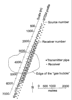
Figure 4 is a schematic plan of a typical arrangement of sources and receivers
of a
multichannel transient electromagnetic measurement system over a subsurface
volume
of gas used for performing a method according to the present invention;
Figure 5 shows the electric potential difference between two electrodes a few
cm apart
and a few cm from a 250 m long current dipole source;
Figure 6 shows normalised system responses for 8 A, 16 A and 32 A source
currents
showing the non-linearity of the system response with current;
Figure 7 is a typical in-line gradient of the electric potential response to a
step in
current at the source;
Figure 8 shows a single approximate earth impulse response for a source-
receiver
separation of 1 km;
Figure 9 shows a 1 km common-offset section of the derivative of the
approximate
earth response for data relating to measurements at the site shown in Figure 3
taken in
1994;
Figure 10 shows a 1 km common-offset section of the derivative of the
approximate
earth response for data relating to measurements at the site shown in Figure 3
taken in
1996; and
Figure 11 shows a common-offset section of the 1996 earth impulse responses
subtracted from the 1994 earth impulse responses, with 1 km offset.
Modes for Carrying Out the Invention
Multichannel Transient ElectroMagnetic (MTEM) data can be acquired in a number
of
different ways. By way of example only, there is described below elements of
the data
acquisition system, as used in the THERMIE project OG/0305/92/NL-UK, and as
described
in [14] above. Figure 1 shows a typical configuration of a source and a line
of receivers. The
source is a current in a wire grounded at each end; in this case the two ends
are 250 m apart.
The receivers are represented as boxes in Figure l, each with two channels,
and are spread
out over a line 2 km long, which, in this case, is in line with the source.
The receivers
measure two kinds of electromagnetic response: potential differences, and the
rate of change
of the magnetic field. Potential differences are measured between two grounded
electrodes,
typically 125 m apart, while the rate of change of the magnetic field is
measured with loops
of wire, typically 50 m by 50 m square loops with many turns. Figure 1 shows
thirty-two
receivers: sixteen in-line potential difference receivers, eight cross-line
potential difference
receivers, and eight loops measuring the rate of change of the magnetic field.
The loops
CA 02452215 2003-12-24
WO 03/023452 PCT/GB02/04121
7
alternate down the line with the cross-line receivers. (This configuration was
the result
of constraints imposed by the limited number of two-channel recording boxes
and the
distance over which signals could be transmitted from these units to the data
storage disk on
the computer.) The source can be positioned outside or within the receiver
spread and, in
practice, the source or the receiver spread, or both, can be moved, depending
on the
application. The recorded transient responses from the receivers are suitably
downloaded to
the hard disk, or other storage medium, of a computer.
Choosing x. as the in-line coordinate, y as the cross-line coordinate, and z
as the vertical
coordinate a notation for the measurements is developed. A receiver position
can be denoted
xr = (x"y"z,), and a source position can be denoted xs =(xs,ys,zs).
Figure 2 shows schematically the relationship between the current input (shown
here as an
instantaneous change in polarity) and the expected response. Ex is the
potential difference
in the in-line or x-direction, and ~ ~ is the rate of change of the vertical
component of the
magnetic field, measured with a horizontal loop. From Figure 2 it can be seen
that these
responses vary with time after the current polarity is reversed at the source.
In practice each
of these quantities varies with the source position and the receiver position.
The key to the solution of the problem is the recovery of the impulse response
of the earth.
The configuration consists of an electromagnetic source, for instance a
current dipole or a
magnetic dipole at a location xs, and a receiver, for instance two potential
electrodes or a
magnetic loop at a location xr . The measurement of the response can be
described as
ak(xs~xr~t)- Sk(xs~xr~t) *g(xs~xr~t)+~k(xr~t)
and it may be repeated many times. In this equation the asterisk * denotes
convolution, and
the subscript k indicates that this is the kth measurement in a suite of
measurements for a
given source-receiver pair; sk (xs, x" t) is known as the system response and
may in principle
be different for each measurement; g(xS, x"t) is the impulse response of the
earth and is
fixed for any source-receiver pair, and ~k (x" t) is uncorrelated
electromagnetic noise at the
receiver and varies from measurement to measurement. This equation must be
solved for the
impulse response of the earth g(xs, xr, t) . To do this, the system response
sk (xs, x" t) must
b a known.
In the acquisition and processing of the data to recover the impulse response
of the earth,
there are three critical steps which are formulated here for the first time.
These are:
1. measurement of the system response for each source-receiver pair and in
principle for
each transient;
2. deconvolution of the measured signal for the measured system response to
recover an
estimated impulse response of the earth for each source-receiver pair and in
principle for
each transient; and
3. stacking of these estimated impulse responses to improve the signal-to-
noise ratio and
obtain an improved estimate of the earth impulse response for each source-
receiver pair.
These steps are now described.
CA 02452215 2003-12-24
WO 03/023452 PCT/GB02/04121
8
1. Measurement of the System Response
The system response sk(xs, xr,t) should be determined by measurement in the
fzeld. This
depends on the source position xs and the position x~ of the receiver and may
also
depend on the number k of the transient in the sequence, particularly if there
are
synchronisation problems. There are several ways in which the system response
can be
measured. In the case of the current dipole source shown in Figure 1, the
measurement of
the system response for the electric field could be made with two electrodes
placed very
close (of the order of a few cm) to the source, with the known distance
between them
very small (of the order of a few cm), to avoid generating voltages that are
too large. For
the magnetic field system response, a small horizontal loop could be placed
close (of the
order of a few cm) to the source. Another possibility is to measure the input
current
directly. The recording system used to measure the system response should,
preferably,
have the same characteristics as the system used to record the measurement ak
(xs, Xr, t)
described by equation (1) and, if the recording is digital, it should be
unaliased. If the
recording systems are not identical, the transfer function between the two
must be known,
so that differences can be eliminated. This is seen as follows.
The recording instrument used to measure the system response at the source has
an
impulse response r(XS, t) , which must be known, while the recording
instrument used to
make the measurement ak (xs, xr, t) at the receiver has a response r(xr, t) ,
which must
also be known. Then the response r(xr,t) can be related to the response
r(xs,t) by the
equation,
Y(Xr~t) = y(xs~t)* ~(xs~Xr~ t)~
in which the asterisk * represents convolution, and f (Xs,xr,t.) is the
Fourier transform of
the transfer function relating the two responses. If the time function of the
input signal at
the source is hk(xs,t), then the system response required to solve equation
(1) is
sk(Xs, Xr,t)= ylk(Xs,t)*Y(Xr,t). (3)
The system response measured with the receiving means and recording system at
the
source will be
Sk(Xs~ Xs~t) _ ~'lk(Xs~t)*Y(xs~t).
The system response required to solve equation (1) is obtained from equations
(2), (3) and
(4) as
Sk(Xs~ Xr~t) - Sk(xs~Xs~t)* f (Xs~Xr~t)~
2. Deconvolution
The earth impulse response g(xs, xr,t) can be estimated, with noise, from
equation (1) by
deconvolution, given the known impulse response sk (XS, xr, t) . That is, an
estimate
CA 02452215 2003-12-24
WO 03/023452 PCT/GB02/04121
9
gk(xs,x"t) of the earth impulse response is obtained by deconvolution of
equation (1).
For example, gk(xs,xr,t) may be obtained as the least-squares Wiener filter
that, when
convolved with the known function sk (xs, xr, t) , gives the known function ak
(xs, x" t) .
Any uncertainties in the time origin of the response are resolved
automatically by this
deconvolution step, provided the system response sk(xs, x,,t) and the
measurement
ak (xs, xr, t) are properly synchronised. Synchronisation is important because
the time
parameter t has the same origin in all the four functions (ak(xs,xr,t),
s~.(xs,x,,t),
g(xs,xr,t), and nk(x"t)) of equation (1).
3. Stacking
To improve the signal-to-noise ratio, using a suite of measurements in which k
varies
from 1 to ~, say, a better estimate of g(xs, x,, t) may be made by stacking.
That is, the
improved estimate is
1"
g(xs~ xr~ t) - -~gk (xs~ xr~ t) ~ (6)
~ k=1
Subsequent processing of the estimated impulse responses g(xs, xr, t) and
display of the
results for different source-receiver pairs can use many of the methods
commonly used for
seismic exploration data.
If the system response sk (xs, xr, t) is identical for all ~ measurements made
for the given
source-receiver pair, the stacking can be done first and the deconvolution
afterwards.
The impulse response of the earth g(xs, xr, t) is typically only a few
milliseconds, or tens of
milliseconds, in duration. Therefore, in principle, thousands of repeat
measurements of the
response may be made in a few minutes.
The invention is illustrated in the following non-limitative example.
Within the European Commission THERMIE Project OG/0305/92/NL-UK [14], MTEM
data
sets were obtained in 1994 and 1996 over a gas storage reservoir at St.
Illiers la Ville in
France. Figure 3 shows a schematic section through the underground gas storage
reservoir
and shows the reservoir and monitoring wells. Figure 4 shows a plan of the
MTEM profile in
relation to the edge of the underground "gas bubble". The equipment that was
used to record
the responses ak (xs,xp, t) consisted of sixteen two-channel TEAMEX boxes
manufactured by
Deutsch Montan Technologie. At the time the data were acquired it was not
recognised that
it was necessary to record the system response for each source-receiver pair.
In fact, with
this equipment, it would have been impossible to measure the system response
properly,
because the low-pass filters were insufficient to prevent aliasing of the data
at the 1 ms
sample interval used in recording.
CA 02452215 2003-12-24
WO 03/023452 PCT/GB02/04121
The source input to the ground was essentially a change in polarity of a
current
of approximately 30 amperes, produced by a generator and Zonge transmitter in
a wire 250 m
long, grounded at each end. In fact, the source time function was not a
perfect step, and there
were small oscillations that could be seen on the few aliased measurements of
the system
response that were made in 1996. One of these can be seen in Figure 5. It was
noticed that
the system oscillations varied with the current level, which varied with the
source position.
Figure 6 shows a magnification of the measured system response for three
different current
levels, normalised to the maximum value. It can be seen that the oscillations
differ with
current level. In other words, with hindsight, we see that the system response
was, in
principle, different for every source-receiver pair, and ought to have been
measured. In fact,
we could not have made this measurement with the available equipment.
A typical measurement ax (xs, xr, t) is shown in Figure 7.
The deconvolution step 2 is impossible to apply to these data because the
system response for
each source-receiver pair was not measured (step 1). To create an approximate
estimate of
the impulse response function we argue that the response ak (xs, x" t) is
approximately the
response to a step:
ak(xs~x~'t)~ H(t) *~(xs=xr~t)~
in which H(t) is the Heaviside, or step function. This approximation ignores
the oscillations
observed in the system responses shown in Figure 6. Differentiating both sides
of equation
(7) yields
~ak (x s ~ x n t) Ul1 (t)
C~t N (~Jt ~(xs' x r' t)
S(t) * 8'(~s~ xr~ t)
g(xaa~r~t)~
That is, the derivative of the measured response is approximately equal to the
impulse
response of the earth. These estimated impulse responses had synchronisation
errors of the
order of ~3 ms. These errors were a fault of the data acquisition system, but
would have been
eliminated if we had been able to measure the system response, as noted above.
In fact, the
timing errors can be estimated because the estimated impulse response has a
very sharp peak
at the beginning, which should arrive at the same time for all responses for
the same source-
receiver pair. Figure 8 shows an estimate of the earth impulse response g(xS,
x" t) , after
stacking the time-corrected earth impulse responses for one source-receiver
pair.
Figure 9 shows a common-offset section of the time derivative of estimated
earth impulse
responses for the 1994 data, in which the source-receiver distance is fixed,
the horizontal
scale is the position of the mid-point between source and receiver, and the
vertical scale is
time. The effect of the increased resistivity over the gas-filled reservoir
can clearly be seen.
Figure 10 shows the corresponding section for the 1996 data. Again, the effect
of the
resistive gas-filled reservoir can clearly be seen. There was a slight
movement of the gas-
water content between October 1994, when the reservoir was full, and August
1996, when it
CA 02452215 2003-12-24
WO 03/023452 PCT/GB02/04121
11
was less full. Subtracting the 1996 earth impulse responses from the 1994
earth
impulse responses yields the difference in response, and shows how the rock
resistivity is
changed by the change in fluid content. Figure 11 shows a common-offset
section of these
differences, and clearly shows that there was more gas in the steeply-dipping
southern part of
the reservoir in 1994.
With this approximate analysis we have shown that it is possible (1) to detect
and locate the
presence of hydrocarbons with the MTEM method, and (2) to monitor the movement
of the
fluids in the reservoir. Given all the approximations that were made to obtain
this result, it is
clear that much better results would be obtained using the method of data
acquisition and
processing of the present invention.
The data should preferably be digitally recorded and processed in a computer
either in real
time or subsequently to create a subsurface representation of resistivity
contrasts.
The MTEM measurements are made on or near the earth's surface which includes
the sea
floor. In the case of measurements at or near the sea floor, measurements may
be made in the
sea close to the actual seabed in view of the conductive nature of the
seawater.
It will be appreciated from the above description that a key to the invention
is the
measurement and deconvolution of the system response sk (xs, x,, t) ,
including source-
receiver synchronisation, for every measured transient response ak (xs, xr,
t), as defined in
equation (1). This includes any approximation to this, such as is described
above with
reference to previously obtained data, in which there was an approximation of
the
deconvolution by differentiation of ak(xs,xY,t), the synchronisation errors
found being
subsequently corrected.
The invention also relates to apparatus for mapping subsurface resistivity
contrasts and to a
system for mapping subsurface resistivity contrasts.
Industrial Applicability
The invention finds application in locating and identifying underground
deposits of fluids,
such as hydrocarbons and water.