Note: Descriptions are shown in the official language in which they were submitted.
CA 02468932 2004-05-27
WO 03/050984 PCT/IB02/05446
1
POLARISATION MODE DISPERSION COMPENSATOR
The present invention relates to methods of adaptive adjustment of PMD
compensators
in optical fiber communication systems. The present invention also relates to
a
compensator in accordance with said method.
In optical fiber telecommunications equipment the need to compensate the
effects of
polarization mode dispersion (PMD) which occur when an optical signal travels
in an
optical fiber based connection is known.
It is known that P1VID causes distortion and dispersion of optical signals
sent over
optical fiber connections making the signals distorted and dispersed. The
different time
delays among the various signal components in the various polarization states
acquire
increasing importance with the increase in transmission speeds. In modern
optical fiber
based transmission systems with ever higher frequencies (10 Gbit/s and more),
accurate
compensation of P1VII~ effects becomes very important and delicate. This
compensation
must be dynamic and performed at adequate speed.
The general purpose of the present invention is to remedy the above mentioned
shortcomings by making available a method of fast, accurate adaptive
adjustment of a
P1VVID compensator and a compensator in accordance with said method.
CA 02468932 2004-05-27
WO 03/050984 PCT/IB02/05446
2
In view of this purpose it was sought to provide in accordance with the
present
invention a method for the adaptive adjustment of a PMD compensator in optical
fiber
communication systems with the compensator comprising a cascade of adjustable
optical devices over which passes an optical signal to be compensated
comprising the
steps of computing the Stokes parameters S0, S 1, S2, S3 in a number Q of
different
frequencies of the signal output from the compensator, producing control
signals for
parameters of at least some of said adjustable optical devices so as to make
virtually
constant said Stokes parameters computed at the different frequencies.
In accordance with the present invention it was also sought to realize a PN~
compensator in optical fiber communication systems applying the method and
comprising a cascade of adjustable optical devices over which passes an
optical signal
to be compensated and an adjustment system which takes the components yl(t)
and y~(t)
on the two orthogonal polarizations at the compensator output with the
adjustment
system comprising a controller which on the basis of said components taken
computes
the Stokes parameters So, S1, S2, S3 in a number Q of different frequencies of
the signal
output from the cornpensator and which emits control signals for at least some
of said
adjustable optical devices so as to make virtually constant the Stokes
parameters
computed at the different frequencies.
To clarify the explanation of the innovative principles of the present
invention and its
advantages compared with the prior art there is described below with the aid
of the
annexed drawings a possible embodiment thereof by way of non-limiting example
applying said principles. In the drawings -
CA 02468932 2004-05-27
WO 03/050984 PCT/IB02/05446
3
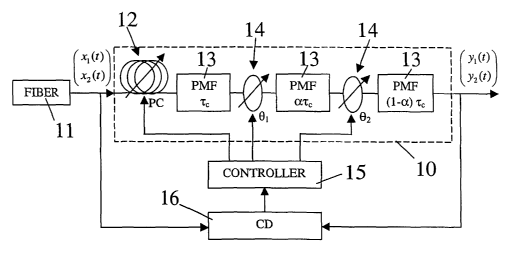
FIG 1 shows a block diagram of a PMD compensator with associated control
circuit,
and
FIG 2 shows an equivalent model of the PMD compensator.
With reference to the FIGS FIG 1 shows the structure of a P1V1D compensator
designated as a whole by reference number 10. This structure consists of the
cascade of
some optical devices which receive the signal from the transmission fiber 11.
The first
optical device is a polarization controller 12 (PC) which allows modification
of the
optical signal polarization at its input. There are three polarization
maintaining fibers
13 (PMF) separated by two optical rotators 14.
A PMF fiber is a fiber which introduces a predetermined differential unit
delay (DGD)
between the components of the optical signal on the two principal states of
polarization
(PSP) termed slow PSP and fast PSP.
In the case of the compensator shown in FIG 1 the DGD delays at the frequency
of the
optical carrier introduced by the three PMFs are respectively i~, ai~ and (1-
a) i~ with
0<a<1 and with i~ and a which are design parameters.
An optical rotator is a device which can change the polarization of the
optical signal
upon its input by an angle 8; (the figure shows ~i for the first rotator and
~~, for the
second) on a maximum circle on the Poincare sphere.
CA 02468932 2004-05-27
WO 03/050984 PCT/IB02/05446
4
An optical rotator is implemented in practice by means of a properly
controlled PC.
In FIG 1, xl(t) and x2(t) designate the components on the two PSPs of the
optical signal
at the compensator input whereas similarly yl(t) and y2(t) are the components
of the
optical signal at the compensator output.
The input-output behavior of each optical device is described here by means of
the so
called Jones transfer matrix H(w) which is a 2 x 2 matrix characterized by
frequency
dependent components. Designating by Wl(c~) a W~(cu) the Fourier transforms of
the
optical signal components at the device input the Fourier transforms Zl(c~) a
ZZ(eo) of
the optical signal components at the device output are given by:
Zi(Ct~) =H(Cr~) Wi(CU) (1)
ZZ (CO) Wi (CV)
Thus the Jones transfer matrix of the PC is:
~ ~ (2)
_ hz ~*
where hl a h2 satisfy the condition ~hl~a+~h2~2 =1 and are frequency
independent.
Denoting by cal and ~2 the PC control angles, hl and h2 are expressed by:
hl=-cos(~2-~1)+ j sin(~2-y) sin~l (3)
h2= j sin(~a-y) cosy
CA 02468932 2004-05-27
WO 03/050984 PCT/IB02/05446
Clearly if the PC is controlled using other angles or voltages, different
relationships will
correlate these other parameters with hl and h~. The straightforward changes
in the
algorithms for adaptive adjustment of the PMD compensator are discussed below.
5 Similarly, an optical rotator with rotation angle 9; is characterized by the
following
Jones matrix:
cos 6; sin 6; (4)
-sin~; cos~;
0
The Jones transfer matrix of a PMF with DGD i; may be expressed as RDR-1 where
D
is defined as:
a jeirc; ~z
D= _
0 g ~2 (5
and R is a unitary rotation matrix accounting for the PSPs' orientation. This
matrix R
may be taken as the identity matrix I without loss of generality when the PSPs
of all the
PMFs are aligned.
As shown in FIG 1, to control the PMD compensator a controller 15 is needed to
produce optical device control signals of the compensator computed on the
basis of the
quantities sent to it by a controller pilot 16 termed controller driver (CD).
CA 02468932 2004-05-27
WO 03/050984 PCT/IB02/05446
6
The CD feeds the controller with the quantities needed to update the
compensator
optical device control parameters. As described below, these quantities will
be
extracted by the CD from the signals at the input andlor output of the
compensator.
The controller will operate following the criterion described below and will
use one of
the two algorithms described below.
To illustrate the PMD compensator adaptive adjustment algorithms let us assume
that
the controller can directly control the parameters ~1, ~2, 61 and 0a which we
consolidate
in a vector 8 defined as:
e-(~1~~2~ela~2~
If it is not so, in general there will be other parameters to control, for
example some
voltages, which will be linked to the previous ones in known relationships.
The time instants in which the update of the compensator parameters is
realized are
designated tn (con n=0,1,2...,), and Tll designates the time interval between
two
successive updates, thus tn+i=tn+Tu. In addition, ~(tn) designates the value
of the
compensator parameters after the nth update.
In accordance with the method of the present invention the criterion for
adjusting the
compensator parameters employs the so-called Stokes parameters. Computation of
the
Stokes parameters for an optical signal is well known to those skilled in the
art and is
not further described.
CA 02468932 2004-05-27
WO 03/050984 PCT/IB02/05446
7
Again in accordance with the method the parameters A of the compensator are
adjusted
to make constant the Stokes parameters computed at different frequencies on
the
compensator output signal. The four Stokes parameters So, S1, S2 a S3 computed
at the
frequency f~ are designated by:
So ~f=f. = So,~
Sl ( f= fl = Sl,~
Sz ~f=f~ - Sz,t
S3 I f= f~ - S3,1
Similarly, the Stokes parameters computed at the frequency fp are designated
by So,P,
SI,Pa S2,P a s3,p~
Using these Stokes parameters the following unitary vectors are constructed
with
components given by the three Stokes parameters S1, S2, S3 normalized at the
parameter
So. (.)Tbelow designates the transpose while (.)* designates the complex
conjugate:
T
'Sl.l 'S2,1 _s3,1
a a a
'So,1 'SO,I 'So,l
and
T
S1,P 'SZ,P 'S3,P
a a a
'SO,P 'SO,P '~o,P
In the absence of P1VE? these two vectors are parallel. Consequently, if their
quadratic
Euclidean distance is considered G1P(~):
CA 02468932 2004-05-27
WO 03/050984 PCT/IB02/05446
z z z
G (~) _ _Si,t - Si,p + sz,t _ Sz,n + ss,t _ S3,n ( )
So,t So,p so,t so,p so,t so,p
which is a function of the parameters 0 of the PMD compensator it will be zero
when
the PMD is compensated at the two frequencies considered ft and fp.
Now consider a number Q of frequencies ft, l=1,2,...,Q. Compute the Stokes
parameters
at these frequencies and construct the corresponding units defined as
explained above,
i.e. with components given by the three Stokes parameters S1, S2, S3
normalized with
respect to the parameter So. All these units are parallel if and only if the
sum of their
quadratic Euclidean distances is zero.
Consequently, to adaptively adjust the P1V~ compensator parameters we define
the
function G(6) which is to be minimized as the sum of the quadratic distances
GlP(e)
with l,p =1,2,...,Q, i.e. the surn of the quadratic distances of the pair of
vectors at the
different frequencies ft and fp, for l,p=1,2,...Q:
~ t-t
G(0) - ~ ~ Gtp (0) (7)
L=2 p=1
The update rule for the compensator parameters to be used in accordance with
the
present invention are:
CA 02468932 2004-05-27
WO 03/050984 PCT/IB02/05446
9
,~, ,/, aG(6) Q f-1 aGfp (e)
Y'1 (tn+1 ) - Y'1 (tn ) - y ' - ~1 (fin ) - Y ,/,
~~1 a = e(tn ) f=z P=1 ~~1 ~ = e(tn )
,/, ,~ aG(e) , Q f-1 aGfp (e)
~2 (tn+1 ) - Y'2 (tn ) ' Y ~1 - y'2 (tn ) ,~
~~2 a = ~(tn ) f=2 p=1 ~~2 a = 8(tn )
(8)
~ t _ _ ~G 8 - ~1 (tn )
1 ( n+1 ) ~1 (tn ) ~ ~ ~ ~ 1=2 p=1 1
1 a - e(tn ) a = e(tn )
__ _ aG(~) ~ f-1 aGfp (e)
~2 (tn+1 ) ~2 (tn ) Y ~ - e2 (tn )
1182 a = e(t ) f=2 p=_1 (~~2 ~ _
n n
where ~0 is a scale factor which controls the amount of the adjustment.
In vector notation this means that the vector of the compensator parameters is
updated
by adding a new vector with its norm proportionate to the norm of the gradient
of G(8)
and with opposite direction, i.e. with all its components having their sign
changed. This
way, we are sure to move towards a relative minimum of the function G(A).
All this is equivalent to:
Q f-1 (9)
e(tn+1 ) = e(tn ) - y vG(~)Ie = ~(tn ) = e(tn ) ~~ ~ ~Gfp (e)I a = ~(tn )
~o
A simplified version of (9) consists of an update by means of a constant norm
vector
and therefore an update which uses only the information on the direction of
VG(9) . In
this case the update rule becomes.
CA 02468932 2004-05-27
WO 03/050984 PCT/IB02/05446
~I~ocp (e)le - ~ t (lo)
e(tn+I ) _ ~(tn ) 'ysign OG(~)I = 6(t" ) 'yszgn
j2 I=2 p=1 ( n )
where sign (z) designates a vector with unitary components and of the same
sign as the
5 components or the vector z.
Two methods are now described for computing the gradient of the G(~) function
and
obtaining the required control parameters.
10 First Method
To implement the update rules (8) the partial derivatives of G(8) for 8 = A
(tn) can be
computed using the following five-step procedure.
- Step 1. find the value of G[8(tn)]=G[~1(tn), ~Z(tn), ~1(tn), 9~(tn)] at
iteration n. To
do this, in the time interval (tn, tn+Tu/5) the Stokes parameters at the above
mentioned Q
frequencies are derived and the value of the function G(8) is computed using
equations
(6) and (7) .
- Step 2. find the partial derivative
ac(e)
at iteration n. To do this, parameter cal is set at ~1(tn)+0 while the other
parameters are left unchanged. The corresponding value of G(8), i.e.
G[~1(tn)+0, ~~(tn), 91(tn), 62(tn)], is computed as in step 1 but in the time
interval
CA 02468932 2004-05-27
WO 03/050984 PCT/IB02/05446
11
(tn+Tu/5, tn+2Tu/5). The estimate of the partial derivative of G(8) as a
function of
~1 is computed as:
aG(e) ~L~I(tn)+~~~2(tn)sel(tn),e2(tn)J-GL~1(tnO~2(tn)sel(tn)se2(tn)J (11)
s
- Step 3. Find the partial derivative:
aG(6)
aY°2 a = 8(tn )
at iteration n. To do this the parameter ~2 is set at ~2(tn)+D while the other
parameters are left changed. The corresponding value of G(6), i.e. G[~1(tn),
~2(tn)+~, 81(tn), 82(tn)], )], is computed as in step 1 but in the time
interval
(tn+2Tu/5, tn+3Tu/5). The estimate of the partial derivative of G(~) with
respect
to ~2 is computed as:
UG(e) ~~~1 ~tn ~~ Y°2 ~tn ) + ~~ el (tn )s e2 ~tn ~~ GLY'1 ~tn )s Y'2
~tn )~ ~1 ~tn )s e2 ~tn )~
a~ _ 0 (12)
~ = e(tn )
- Step 4: Find the partial derivative:
~o aG(e)
8 = e(tn )
at iteration n. To do this, parameter 81 is set at ~1(tn)+ ~ while the other
parameters are left unchanged, the corresponding value of G(8), i.e. G[~1(tn),
~z(tn), 61(tn)+0, 6~(tn)], is computed as in Step 1 but in the time interval
CA 02468932 2004-05-27
WO 03/050984 PCT/IB02/05446
12
(tn+3Tu/5, tn+4T"/5) and the estimate of the partial derivative of G(0) with
respect to 91 is computed as:
aG(8) GLY'I (tn )s Y'2 (tn )s el (tn ) + ~a e2 (tn )J- GLY'1 (tn )s Y°2
(tn )s ~1 (tn )s e2 (tn )J
ael a = e(tn) ~ (13)
- Step 5: Find the partial derivative:
aG(6)
ae2 e=e(tn)
at iteration n. To do this the parameter ~a is set at ~2(tn)+O while the other
parameters
are left changed. The corresponding value of G(8), i.e. G[~1(tn), c~2(tn),
61(tn), 92(tn) +0],
is computed as in step 1 but in the time interval (tn+4Tu/5, tn+T"). The
estimate of the
partial derivative of G(A) with respect to ~2 is computed as:
7G(9) GLY°1 (tn )s Y'2 (tn O 81 (tn )s e2 (tn ) + 0~- G~~i (tn )s'f'2
(tn )~ el (tn )s ~2 (tn )J (14)
3 BZ 4
8 = ~(tn )
The above parameter update is done only after estimation of the gradient has
been
completed.
Note that in this case it is not necessary that the relationship between the
control
parameters of PC and optical rotators and the corresponding Jones matrices be
known.
Indeed, the partial derivatives of the function with respect to the
compensator control
parameters are computed without knowledge of this relationship. Consequently
if the
control parameters are different from those assumed as an example and are for
example
CA 02468932 2004-05-27
WO 03/050984 PCT/IB02/05446
13
some voltage or some other angle, we may similarly compute the partial
derivative and
update these different control parameters accordingly.
Lastly, it is noted that when this algorithm is used the CD must receive only
the optical
signal at the compensator output and must supply the controller with the
Stokes
parameters computed at the Q frequencies f1, l=1,2,...,Q.
Second method
When an accurate characterization of the PC and of each optical rotator is
available the
update rules can be expressed as a function of the signals on the two
orthogonal
polarizations at the compensator input and output.
In this case, for the sake of convenience it is best to avoid normalization of
the three
Stokes parameters S1, S2 a S3 with respect to So and use the function H(8)
defined as:
FI (6) ~ ~ FI p (0) (15)
l=2 p=1
where
HlP(~)=(s 1,1's 1.P)2+(s2,1-S2,P)2+(s3,1'S3~P)2 ( 16)
Consequently we have new update rules similar to those expressed by equation
(8) or
equivalently (9) with the only change being that the new function H(~) must
substitute
the previous G(~).
CA 02468932 2004-05-27
WO 03/050984 PCT/IB02/05446
14
Before describing how the gradient of this new function H(8) is to be computed
let us
introduce for convenient an equivalent model of the PMD compensator.
Indeed it was found that the PMD compensator shown in FIG 1 is equivalent to a
two-
dimensional transversal filter with four tapped delay lines (TDL) combining
the signals
on the two principal polarization states (PSP). This equivalent model is shown
in FIG 2
where:
cl = cos ~1 cos ~zh~
ez = -sin Bl sin 9z1~
c3 = -sin ~1 cos Bzhz
c4 = -cos ~I sin Bzlr~
CS = COS ~1 cOS 82~ 17)
c6 = -sin ~1 sin 8z1~
c~ "-- sin 91 cos ~zh,"
eg = cos ~1 sin 9zlzi
is
For the sake of convenience let c(8)designate the vector whose components are
the cl in
(17). It is noted that the tap coefficients ci of the four TDLs are not
independent of each
other. On the contrary, given four of them the others are completely
determined by
(17). In the FIG for the sake of clarity it is designated (3=1-a.
The gradient of H~p(A) with respect to 8 is to be computed as follows:
OFI ~~ (8) = 4(Sl,l - Si,n ) Re ~ ~~~~~ yt (t)ai (t) - Yz,t (t)bi (t) - Yi P
(t)a P (t) + Yz,n (t)b ~ (~)~ dtJ
+ 4(Sz,~ - Sz,~ ) Re ~ ~~n~~ [Yz,t (t)ai (~) + Yi,t (t)~i (t) - Yz,n (t)an (t)
- Yi ~ (t)b j (~)~ dtJ
Ja
- 4(Ss.t - Ss,n ) ~ Tu ~n"+I [Yz,r (t)ai (t) + Yi,i (t)bi (t> - Yz,~ (t)a P
(~) - Yi ~ (t)b p (t)~ dtJ
CA 02468932 2004-05-27
WO 03/050984 PCT/IB02/05446
where:
- yl,~(t) and y2,1(t) are the signals yi(t) and ya(t) at the compensator
output
respectively filtered through a narrow band filter centered on the frequency
fi (similarly
for yl;p(t) and ya,p(t));
5 - al(t) and bl(t) are the vectors:
xl,l (t) x2,1 (t -
~2~ )
xl,l (t - xz,l (t -
aZ~ ) z~ - ~z~
a
x~,t (t - xz,l (t -
~~ ) z~ )
a t = xll (t z~ bl (t) xz,l (t -
( ) G~2c ) - ~Z~ )
*
! x (t) - x
z,l (t - Zz
i l
10 xz,l (t - - xl ~ (t
ex2-~ ) - z~ - ~z~
xz,l(t-z~) -xl(t-z~)
xz,l (t - - xl,l (t
z~ - ~z~ - ~~~ )
)
with xl,L(t) and x2,1(t) which are respectively the signals xl(t) and x2(t) at
the
compensator input filtered by a narrow band filter centered on the frequency
fl
15 (similarly for yl,p(t) and y~,p(t));
- J is the Jacobean matrix of the transformation c=c(8) defined as
_a~l _a~i a~l a~l
ail a~2 a~1 ae2
_a~2 _a~2 a~2 a~2
a~2 ae, ae2
a~$ _a~$ a~g a~$ (18)
ail a~2 a~1 ae2
The parameters 8 are updated in accordance with the rule
Q r-! (19)
8(tn+1 ) = e(tn ) - ~~ ~ v~lP (e)I ~ = 8(t
!-_2 P-1 n )
CA 02468932 2004-05-27
WO 03/050984 PCT/IB02/05446
16
or in accordance with the following simplified rule based only on the sign:
8(t = 8 ~~~OH~P (0)I
n+1 ) (tn ) YSl~f2 1_2 p=I ~ = 0(tn ) 20
When the control parameters are different from those taken as examples we will
naturally have different relationships between these control parameters and
the
coefficients c;.
For example, if the PC is controlled by means of some voltages, given the
relationship
between these voltages and the coefficients hl and h2 which appear in (2), by
using the
equations (17) we will be able to express the coefficients c; as a function of
these new
control parameters.
Consequently in computing the gradient of the function H(8), the only change
we have
to allow for is the expression of the Jacobean matrix 3, which has to be
changed
accordingly.
Lastly it is noted that when this second method is used the CD must receive
the optical
signals at the input and output of the compensator. The CD must supply the
controller
not only with the Stokes parameters for the optical signal at the compensator
output and
computed at the Q frequencies fl, l=1,2,...,Q but also with the signals
xl,l(t), x2,1(t), yr,a(t)
a y2,~(t) corresponding to the Q frequencies fl, l=1,2,...,Q.
CA 02468932 2004-05-27
WO 03/050984 PCT/IB02/05446
1~
It is now clear that the predetermined purposes have been achieved by making
available
an effective method for adaptive control of a PMD compensator and a
compensator
applying this method.
Naturally the above description of an embodiment applying the innovative
principles of
the present invention is given by way of non-limiting example of said
principles within
the scope of the exclusive right claimed here.