Note: Descriptions are shown in the official language in which they were submitted.
CA 02481627 2008-10-07
1
io Method and device for continuous monitoring of the
concentration of an analyte
The present invention relates to a method and a device
for continuous monitoring of the concentration of an
analyte by determining its change over time in the living
body of a human or animal. The term "continuous
monitoring (CM)" is used hereafter for this purpose.
A CM method and device is described, for example, in
(1) US Patent 5,507,288.
A main task is the continuous monitoring of the
concentration of glucose in the body of the patient,
which is of great medicinal significance. Studies have
led to the result that extremely grave long-term effects
of diabetes mellitus (for example, blinding because of
retinopathy) can be avoided if the change over time of
the concentration of the glucose is continuously
monitored in vivo. Continuous monitoring allows to dose
the required medication (insulin) precisely at each point
in time and to keep the blood sugar level always within
narrow limits, similarly to a healthy person.
DOC'SM"iL: 1 586077\1
CA 02481627 2007-04-24
-2-
The present invention relates in particular to CM of
glucose. Further information can be taken from document
(1) and the literature cited therein.
The present invention is, however, also suitable for
other applications in which the change over time of an
analyte in the living body (useful signal) is derived
from a measurement signal, which comprises measurement
values, measured at sequential points in time, of a
measurement variable correlating with the concentration
desired. The measurement signal may be measured
invasively or non-invasively.
An invasive measurement method is described, for
example, in
2) US Patent 6,584,335.
Here a hollow needle carrying a thin optical fiber is
stuck into the skin, light is irradiated under the skin
surface through the optical fiber, and a modification
of the light through interaction with interstitial
liquid which surrounds the optical fiber is measured.
In this case, the measurement signal comprises
measurement values obtained from light which is
returned through the optical fiber into a measurement
device after the interaction. For example, the
measurement signal may comprise spectra of the light
which are measured at sequential points in time.
Another example of invasive measurement methods is the
monitoring of concentrations by means of an
electrochemical sensor which may be stuck into the skin.
An electrical measurement variable, typically a current,
CA 02481627 2004-09-15
3
is thus determined as the measurement variable which is
correlated with the concentration of the analyte.
Different non-invasive methods are discussed in Document
(1). These include spectroscopic methods in which light
is irradiated directly (i.e., without injuring the skin)
through the skin surface into the body and diffusely
reflected light is analyzed. Methods of this type have
achieved some importance for checkincr the change over
time of oxygen saturation in the blood. For the analysis
of glucose alternative methods are preferred, in which
light is irradiated into the skin in a strongly localized
manner (typically punctually) and the useful signal
(course of the glucose concentration) is obtained from
the spatial distribution of the secondary light coming
out of the skin in the surroundings of the irradiation
point. In this case the measurement signal is formed by
the intensity profile, measured at sequential points in
time, of the secondary light in the surroundings of the
irradiation point.
A common feature of all methods of this type is that the
change of the concentration over time (useful signal) is
determined from the measurement values measured at
sequential points in time (measurement signal) using a
microprocessor system and a suitable algorithm. This
analysis algorithm includes the following partial
algorithms:
a) a filter algorithm, by which errors of the useful
signal resulting from signal noise contained in the
measurement signal are reduced and.
b) a conversion algorithm, in which a functional
relationship determined by calibration, which
relationship describes the correlation between
measurement signal and useful signal, is used.
CA 02481627 2008-02-01
4
The Conunissioner of Patents
The Examiner maybe inclined to consider the "measurement noise matrix" R(i)
as a signal variation parameter. Upon review of figure 3D of Knobbe et al.
giving a
recursion equation for calculating the Kalman gain. This equation corresponds
to
equation (6) of the instant patent application, wherein R(i) of Knobbe et al.
corresponds
to the measurement error covariance matrix V of the application. However, R(i)
of
Kalman et al. is not a quantity the determination of which depends on the
actual point
of time. It is also not a quantity which depends on the measurement signal,
even less is
it a quantity for signal variations which are determined from measurement
values
including values detected during the preceding 30 minutes.
In the description of Knobbe et al. the measurement noise matrix is assumed to
have a constant value R (see figure 3B of Knobbe et al., last line on the left
side). The
same is also true with respect to the values of an exemplary embodiment shown
in the
same drawing giving constant values 152 and 52 respectively which are assumed
for the
time periods "before 20 hours" and "after 20 hours". The same constant values
may be
found in the program codes shown in table 4 on page 19 of Knobbe et al. as
well as on
page 10 (lines 1 and 4).
Nowhere in Knobbe et al. is there any description of an equation or other
information allowing calculation of a time-dependent changing value of R, let
alone the
possibility to adapt this value dynamically depending on changes of the
measurement
signal over time.
There is also no reason to use a quantity of R which changes over time
because,
in Knobbe et al., the measurement covariance matrix serves - as usual - to
remove
standard white noise which can be (and generally is) assumed to be constant.
. The latter difference discussed above already indicates that the methodic
aspect
of Knobbe et al. does not relate to the specific application or problem to
reduce the
influence of NNNC-noise.
CA 02481627 2004-09-15
(6) US Patent 5,921,937
(7) EP 0 910 023 A2
5 (8) WO 01/38948 A2
(9) US Patent 6,317,662
(10) US Patent 6,575,905 B2
As noted, the filter algorithm is used for the purpose of
removing noise signals which are contained in the raw
measurement signal and would corrupt the useful signal.
The goal of every filter algorithm is to eliminate this
noise as completely as possible, but simultaneously avoid
to disturb the measurement signal. This goal is
especially difficult to achieve for in vivo monitoring of
analytes, because the measurement signals are typically
very weak and have strong noise components. Special
problems arise because the measuremen.t signal typically
contains two types of noise, which differ significantly
in regard to the requirements for the filter algorithm:
- measurement noise: such noise signal components follow
a normal distribution having a constant standard
deviation around the correct (physiological)
measurement signal
- non-physiological signal changes, which are caused,
for example, by movements of the patient and changes
of the coupling of a measurement sensor to the skin to
which it is connected. They are typically neither
distributed normally around the physiological
measurement signal, nor is the standard deviation from
the physiological measurement signal constant. For
such noise components of the raw signal the term NNNC
(non-normal, non-constant)-noise is used hereafter.
CA 02481627 2008-10-07
6
The present invention is based on the technical problem to achieve a better
precision of CM methods by improving the filtering of noise signals.
According to the present invention this is achieved by means of a filter
algorithm which includes an operation in which the influence of an actual
measurement value on the useful signal is weighted using a weighting factor
("controllable filter algorithm"), a signal variation parameter (related in
each
case to the actual point in time, i.e. time-dependent) is determined on the
basis
of signal variations detected during the continuous monitoring in close
chronological connection with the measurement and the weighting factor is
adapted dynamically as a function of the signal variation parameter determined
for the point in time of the actual measurement.
In one aspect of the invention there is provided a method for continuous
monitoring of an analyte concentration by determining a change over time of
the analyte in a living body of a human or animal, the method comprising:
measuring at sequential points in time, measurement values of a measurement
variable correlating with a desired concentration of the analyte, as a
measurement signal (zt);
determining the change over time of the concentration of the analyte from the
measurement signal as a useful signal (yt) by means of a calibration;
providing a filter algorithm in the time domain for determination of the
useful
signal (yt) from the measurement signal (zt), wherein the filter algorithm
reduces errors of the useful signal resulting from noise contained in the
measurement signal, wherein the filter algorithm includes an operation in
which the influence of an actual measurement value on the useful signal is
weighted by means of a weighting factor (V);
determining a time dependent signal variation parameter (al) related to an
actual point of time on the basis of signal variations detected in close
chronological relation to the measurement of the actual measurement value;
said time dependent signal variation parameter being a measure for signal
variations for a period of time preceding an actual measurement value and
DOCSMTL: 3011343\1
CA 02481627 2008-10-07
6a
being determined on the basis of measurement values including values which
were measured less than 30 minutes before the measurement of the actual
value; and
adapting dynamically the weighting factor as a function of the signal
variation
parameter determined for the point in time of the actual measurement, the
weighting factor being changed in such a direction that the influence of the
actual measurement value is reduced with increasing standard deviation of the
measurement signal.
In another aspect of the invention there is provided a device for continuous
monitoring of a concentration of an analyte by determining a change over time
of the analyte in a living body of a human or animal, the device comprising:
a measurement unit, by which measurement values of a measurement variable
correlating with the desired concentration are measured as the measurement
signal (z) at a sequential points in time;
an analysis unit, by which the change over time of the concentration is
determined by means of a calibration as a useful signal (y) from the
measurement signal, and
a filter algorithm in the time domain for determination of the useful signal
(yt)
from the measurement signal (zt) to reduce errors of the useful signal, which
result from noise contained in the measurement signal;
the filter algorithm including operation, in which influence of an actual
measurement value on the useful signal is weighted using a weighting factor
(V), such that a time dependent signal variation parameter (vt) is determined
on
the basis of signal variations detected in close chronological relationship
with
the measurement of the actual measurement value,
the time dependent signal variation parameter being a measure for signal
variations for a period of time preceding an actual measurement value and
being determined on the basis of measurement values including values which
were measured less than 30 minutes before the measurement of the actual
value; and
DOC SM'1'L: 3011343\ 1
CA 02481627 2008-10-07
6b
the weighting factor being dynamically adapted as a function of the signal
variation parameter determined for the point in time of the actual
measurement,
the weighting factor being changed in such a direction that the influence of
the
actual measurement value is reduced with increasing tgvtgvstandard deviation
of the measurement signal.
The present invention, including preferred embodiments, will be described in
greater detail hereafter on the basis of the figures. The details shown
therein
and described' in the following may be used individually or in combination to
provide preferred embodiments of the present invention.
Fig. 1 shows a block diagram of a device according to the present
invention;
Fig. 2 shows a schematic diagram of a sensor suitable for the present
invention;
Fig. 3 shows a measurement signal of a sensor as shown in Figure 2;
DOCSMTL: 30113431I
CA 02481627 2004-09-15
7
Fig. 4 shows a symbolic flowchart to explain the
algorithm used in the scope of the present
invention;
Fig. 5 shows a graphic illustration of typical signal
curves to explain the problem solved by the
present invention;
Fig. 6 shows a graphic illustration of experimentally
obtained measurement results.
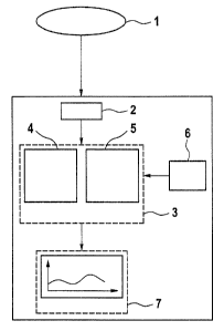
Zo The essential components of a device according to the
present invention are shown in Figure 1. A sensor 1
measures measurement values at sequential points in time.
This measurement signal is transmitted - wirelessly, in
the case shown - to a receiver 2, from which the
measurement signal is further transmitted to an analysis
unit 3, which contains a microprocessor 4 and a data
memory 5. Data and commands may also be transmitted to
the analysis unit 3 via an input unit. 6. Results are
output using an output unit 7, which may include a
display and other typical output means. Of course, the
data processing is performed digitally in the analysis
unit 3 and corresponding converters for converting analog
signals into digital signals are provided. More detailed
explanations are not necessary in this regard, because
the basic construction of devices of this type is known
(from Document 1, for example) and the present invention
is suitable for a wide range of measurement techniques in
which - as explained at the beginning - different
measurement signals correlating to the desired useful
signal are obtained.
Figure 2 shows a sensor 1 in the form of a schematic
diagram, in which an implantable catheter 10 is used in
order to suction interstitial liquid from the
subcutaneous fatty tissue by means of a pump 11. The
CA 02481627 2004-09-15
8
tissue is then suctioned through a photometric
measurement unit 12 into a waste container 13. The line
14 by which the interstitial liquid is transported
contains a transparent measurement cell 15 which is
arranged in the photometric measurement unit 12, into
which primary light originating from a light emitter 16
is irradiated. The secondary light resulting after
passing the measurement cell 15 is measured using a
photodetector 17 and processed by means of a measurement
electronics (not shown) into a raw signal, which - as
shown for exemplary purposes in Figure 1- is transmitted
to an analysis unit 3.
Figure 3 shows the typical graph of a raw measurement
signal as curve A obtained using a sensor as shown in
Figure 2. The intensity I of the secondary light is
measured at a specific wavelength and plotted against the
time t in minutes. Figure 3 is based on a CM experiment
in which the measurement values for curve A were measured
at intervals of one second each.
Variations of the flow of the interstitial liquid from
the body into the photometric measurement unit 12 lead to
regular, relatively small signal variations, which are
referred to as "fluidic modulation". After approximately
three minutes, at the point in time identified with the
arrow 18, an inhibition of the liquid flow occurred,
which may be caused, for example, by movement of the
patient or by the entrance of a cell particle into the
catheter 10. This inhibition of the flow leads to a large
drop of the raw measurement signal A. This is an example
of the fact that not all noise signals are distributed
normally, with essentially constant standard deviation,
around the signal corresponding to the actual
physiological measurement value. Rather also interfering
CA 02481627 2004-09-15
9
contributions of the type shown here exist, for which
these conditions do not apply (NNNC rioise). The object of
the present invention is to perform the required
filtering even in such cases in such a manner that a
useful signal results which corresponds as closely as
possible to the actual physiological concentration of the
analyte. An example for such a useful signal is shown in
Figure 3 as thin line B.
The basis of a filter algorithm operating in the time
domain, which the present invention relates to, is a
system model that describes the change over time of the
variables of interest and their relationship to one
another. The functional relationship which describes the
development of the system from time t: to time t+1 is as
follows:
(1) Yt+i = f t ( Yt. Yt-l . . . . , ut, ut-i . . . . ) =
Therein, yt and ut are vectors, which are referred to as
state vectors and vectors of input variables,
respectively. The state vector yt contains the variables
of physiological interest and optionally check variables,
which allow to check the measurement, as will be
described in greater detail below. In the CM method,
these include the desired analyte concentration, for
example, the glucose concentration gt in the blood. The
speed of change of the analyte concentration gt = dgt/dt
is suitable as a check variable. The state variable yt
may also contain model variables related to the
measurement method. For example, in the case of a
measurement result of the type shown in Figure 3, it is
advantageous to incorporate fluidic modulations into the
system model. These modulations may be described using
their time-dependent frequency cot and the amplitude At,
CA 02481627 2004-09-15
which is also time-dependent. Therefore, four system
variables result for the experiment described on the
basis of Figures 2 and 3: gt,At,wt,gt` .
5 Input variables which, in the field of automatic control,
correspond to control variables and are therefore not
measured themselves are entered into the vector ut. In
the case of glucose monitoring, for example, the
administered insulin quantity given and the bread
10 exchange units supplied are suitable input variables,
because they both influence the glucose concentration in
the blood. If these input variables are used, the vector
ut has two elements: insulin dose and bread exchange
units. A characteristic feature of input variables is
that no prediction of their future values is necessary in
the scope of the filter algorithm.
The mentioned variables of the state vector yt and the
input vector ut are, of course, only to be understood as
examples. The present invention relates to greatly
varying systems which require different system models. It
is not necessary to use the models in a discrete form.
The continuous form with the corresponding differential
equations may also be used.
A characteristic feature of filter algorithms in the time
domain, to which the present invention refers, is that
they include an alternating sequence of predictions and
corrections. A prediction of the system state ("predictor
step") is followed by a subsequent correction of this
prediction on the basis of a further measurement value
("corrector step" ).
CA 02481627 2004-09-15
11
In a predictor step, the actual value of the state
variable yt at the point in time t is predicted using the
system equation (1):
( 2 ) Yt = f t-1 (Yt-1. Yt-2, . . . ; ut-1, ut-2 r . . . ) + wt-1
In this equation, yt identifies the value of the state
vector at the point in time t which is estimated
(predicted) using the data of the previous point in time
(t-1) ; Wt identifies a system error vector.
In the case of a recursive filter algorithm, the
calculation of each predictor step is not performed by
taking all preceding points in time (t-1, t-2, t-3...)
s.s into consideration, but rather by using a weighted sum of
smoothed signal values. In the example of a linear Kalman
algorithm, the corresponding equation may be written as
follows:
(2a) yt = At-lYt-1 + But_1 + wt-1
In this equation, At is the system matrix and B is the
input matrix. In the general (non-linear) case, ft is to
be preset or is to be calculated from data determined up
to this point.
In the corrector step, the prediction is corrected on the
basis of an actual measurement value according to
(3) Yt = at kt + PtOt
In this equation, At is a variable which represents a
measure of the deviation of an actual measurement value
zt from the predicted value and is referred to as the
"innovation".
CA 02481627 2004-09-15
12
(4) At = zt - h(kt)
Further it is taken into consideration that typically the
system variables cannot be observed directly. The linkage
between the measurement values and the state variables is
provided by means of a measurement model (measurement
function ht) according to:
(5) zt = ht(Yt) + vt
The noise of the measurement values is taken into
consideration by vt.
In the case of a linear Kalman algorithm (cf. equation
2a), the measurement equation is
(5a) zt = Ht = Yt + Vt,
Ht referring to the measurement matrix.
For example, in the continuous monitoring of glucose
using an electrochemical sensor, a current i is measured
which is correlated with the glucose concentration gt. In
that example ht describes the correlation of the state
variable gt with the measurement variable i(current),
which is an element of the vector zt.
In the given example of photometric glucose detection
using filter-assisted compensation of the fluidic
modulation, a non-linear measurement model is used which
links the photometric measurement signal zt to the system
variables of glucose concentration gt, amplitude At, and
frequency wt of the fluidic modulation:
zt = gt + At sin (wt=t).
CA 02481627 2004-09-15
13
According to equation (3), the influence of the actual
measurement value (contained in the innovation At) on the
filtered useful signal value yt is weighted by the
factors at and (3t. The described algorithm is therefore
a controllable filter algorithm.
In the case of a Kalman filter, at = 1 for every point in
time and (3t = Kt. Kt refers to the Kalman gain.
Accordingly, the corrector equation is as follows:
(3a) Yt = Yt + KtAt
Further details regarding the Kalman. gain Kt and more
detailed information on the algorithm may be taken from
the relevant literature, as cited above. Expressed
descriptively, the Kalman gain is a m:easure of the weight
given to additional measurement values. The Kalman gain
is calculated anew in every iteration step of the filter
algorithm according to an equation which may be written
in simplified form (for the linear case) as follows:
(6) Kt = Pt = Ht = (Pt=Ht + V) -1
Here, Pt designates the Kalman error covariance matrix. V
designates the measurement error covariance matrix in the
conventional Kalman algorithm.
Equation (6) shows that the elements of Kt may assume
only values between 0 and 1. If the assumed measurement
error V is relatively large in relation to the Kalman
error covariance Pt, Kt is small, i.e., the particular
actual measurement value is given relatively little
weight. In contrast, if V is small in relation to Pt
CA 02481627 2004-09-15
14
(multiplied by Ht), a strong correction occurs due to the
actual measurement value.
Figure 4 shows in graphic form the iteration loop 20
which is the basis of the filter procedure. Alternately a
corrector step which takes an actual measurement value zt
into consideration, and, after a time step dt, a
predictor step for a new point in time are performed. For
example, the corrector step may be calculated according
to equation (3) or (3a) and the predictor step according
to equation (2) or (2a). This part of the algorithm is
referred to as the filter core 22. As explained, it may
be implemented in different ways, as long as it is an
algorithm operating in the time domain and it includes an
operation in which the influence of an actual measurement
value zt on the filter useful signal yt is weighted using
a weighting factor at, (3t, or Kt, respectively.
An important improvement of the filtering is achieved in
the scope of the present invention in that, on the basis
of signal variations detected in close chronological
relationship with the measurement of the actual
measurement value zt, a signal variation parameter,
designated here as 6t, is determined and the weighting of
the influence of the actual measurement value zt is
dynamically adapted in the context of the corrector step
as a function of at. This is shown in graphic form in
Figure 4: box 23 symbolizes the calculation of the
variation parameter 6t as a function of the measurement
signal in a preceding period of time (measurement values
zt_n... Zt) . Box 24 symbolizes the calculation of the
weighting factor taken into consideration in the
corrector step (here, for example, the measurement error
covariance V, which influences the Kalman gain), as a
function of the signal variation parameter 6t. The
CA 02481627 2004-09-15
weighting factor is a time-dependent (dynamically
adapted) variable (in this case Vr).
The present invention does not have the goal of weighting
5 different filter types - like a filter bank - by applying
weighting factors. For this purpose, a series of system
models analogous to equation (2) would have to be
defined, one model for each filter of the filter bank.
This is not necessary in the present invention, whereby
10 the method is less complex.
No precise mathematical rules may be specified for the
functional relationships used in steps 23 and 24, because
they must be tailored to each individual case. However,
15 the following general rules apply:
- The signal variation parameter is determined as a
function of measurement values which have a close
chronological relationship to the particular actual
measurement value. In this way, the speed of adaption
of the filter is sufficient. The determination of the
signal variation parameter is preferably based on
measurement values which were measured less than 30
minutes, preferably less than 15 minutes, and
especially preferably less than 5 minutes before the
measurement of the actual measurement value. At the
least, measurement values from the periods of time
should be included in the algorithm for determining
the signal variation parameter.
- Independently of the equations used in a particular
case, the principle applies that with decreasing
signal quality (i.e., for example, increase of the
standard deviation of the measurement signal), the
signal variation parameter and therefore the weighting
factor (or possibly the weighting factors) are changed
CA 02481627 2004-09-15
16
in such a direction that the influence of the
currently actual measurement value is reduced.
The standard deviation, which may be calculated as
follows, is suitable as the signal variation parameter,
for example.
If one assumes that the determination of the standard
deviation is based on the actual measurement values z and
four 'preceding measurement values zl to z4, and if the
difference between z and the preceding values is referred
to as Sz ((SZn = Z-Zn), the average value s is calculated
as
(7) 6 = 4 (CSZI + SZ2 + CSZ3 + CSZ4)
and the slope cp of a linear smoothing function is
calculated as
3 (9zl - Sz4 ) + Sz2 - 9z3
($) ~ 10
The standard deviation of the four values of the
difference 61, 82, 83, 84 in relation to the linear
smoothing function is
(9) at = [ 3 ($zl - (E + 1,5(p) )2
+ 3(8z2 -( E + 0, 5(p) ) 2
+ 3 (8Z3 -( E - 0, 5(p) Z
+ ~ (Szq - ( E - 1,59) ) 2
CA 02481627 2004-09-15
17
On the basis of this standard deviation at, a dynamic
(time-dependent) measurement error covariance Vt, which
is included in a filter core with the Kalman algorithm,
may be calculated, for example, according to
(10) Vt = (ao + 6t)
In this case, 6o and y are constant parameters which
characterize the filter, and which may be set to tailor
the chronological behavior of the filter, in particular
its adaptivity, to a particular application.
In the example of a controllable recursive filter, the
weighting factors at, pt from equation (3) are a function
of the signal variation parameter in such a manner that
with increasing at, factor at becomes larger and factor
(3t becomes smaller.
As already explained, equations (7) through (10) only
represent one of numerous possibilities for calculating a
signal variation parameter and, based thereon, a
weighting factor for a controllable filter algorithm in
the time domain. The standard deviation, which may, of
course, be calculated using a varying number of
measurement values, can be replaced by variables which
represent a measure for the signal variations in a period
of time preceding an actual measurement value. The term
"signal variation parameter" is used generally to
identify a mathematical variable which fulfills these
requirements.
Three typical graphs of a signal S are plotted against
time t in Figure 5, specifically:
a) as a solid line, a raw signal with strong non-
physiological variations in the time period enclosed
CA 02481627 2004-09-15
18
by circle 25 and oscillates significantly less in the
time period enclosed by rectangle 26, these variations
being essentially physiological.
b) as a dashed line, a useful signal, which was obtained
from the raw signal a) using a Kalman filter, whose
measurement error covariance was set corresponding to
the variation of the raw signal in the circle 25.
c) as a dotted line, a useful signal which was obtained
from the raw signal a) using a Kalman filter, whose
measurement error covariance was set corresponding to
the graph of the raw signal in the rectangle 26.
Evidently, in the case of curve b the strong variations
are filtered well within the circle 25, but in the
is rectangle 26, the signal b reflects the physiological
variations of the raw signal insufficiently. The useful
signal c, in contrast, follows the physiological
variations in the region 26 well, while the filtering of
the non-physiological variations in the region 25 is
insufficient. The conventional Kalman filter algorithm
therefore allows no setting which leads to optimal
filtering for the different conditions shown. In
contrast, the present invention does not even require
knowledge of the maximum variations of measurement
values. The filter algorithm adapts itself automatically
to the changes in the signal course and provides a
filtered signal which corresponds to the curve b in the
circle 25 and to the curve c in the rectangle 26.
Figure 6 shows corresponding experimental results from a
CM experiment for glucose monitoring. A useful signal
resulting from conventional filtering is shown as the
solid curve A (glucose concentration in mg/dl) over the
time in hours. The dashed curve B is the useful signal
CA 02481627 2004-09-15
19
filtered according to the present invention. At the point
in time marked with the arrow 28, the patient begins to
move which interferes with the signal curve. Although
there is very little variation of the free analyte
concentration, the noise caused by the movement (NNNC
noise) cannot be filtered out by the conventional filter.
In contrast, using the filtering according to the present
invention, a useful signal is obtained which approximates
the physiological glucose curve very closely.
Significant additional reliability may be achieved if the
filtering extends not only to the desired analyte
concentration, but rather additionally to at least one
further variable, which is designated "check variable".
This may be a variable derived from the analyte
concentration, in particular its first, second, or higher
derivative versus time. Alternatively, an additional
measurement variable, such as the flow of the
interstitial liquid at the sensor shown in Figure 2, can
be used.
This check variable may, as explained above (for gt', At,
and cot), be included in the filter algorithm as a system
variable. The filtering then also extends to the check
variable, for which corresponding reliable smoothed
useful signal values are available as the result of the
filtering. These may then be compared to threshold
values, in order to perform plausibility checks, for
example. In the case of the glucose concentration, for
example, it is known that the glucose concentration
physiologically does not change by more than 3 mg/dl/min
under normal conditions. A higher filtered value of the
time derivative gt' is a sign of a malfunction. Therefore
the query 30 shown in Figure 4 compares the value of yt'
to a minimum value and a maximum value. The value yt is
CA 02481627 2004-09-15
only accepted as correct if yt' lies within these limits.
Such a comparison would not be possible using the useful
signal A in Figure 6, because the insufficiently filtered
non-physiological variations would lead to false alarms.