Note: Descriptions are shown in the official language in which they were submitted.
CA 02488197 2004-11-30
WO 03/105053 PCT/US03/17803
MARI~OWN MANAGEMENT
BACKGROUND
This description relates to markdown management.
A merchandiser who is planning to sell an item of fashion
merchandise that has a short-life-cycle (for example, a style of
ladies' dress shoes) typically orders an initial inventory of the item
at the beginning of a season, sets an initial retail price, and offers
the item to customers. Because a fashion item will have little value
after the season in which it is offered, the merchandiser watches
the inventory level carefully. If the merchandiser believes that
sales axe not brisk enough to assure that the full inventory will be
sold by the end of the season at the initial full price, he will reduce
the price one or more times during the season with the goal of
increasing the demand in order to clear out the inventory.
Decisions about such markdown prices (called markdown
management) directly affect the retailer's profit.
The success of markdown management is sometimes measured by
the direction and degree of change of sales and gross profit dollars
from one year to the next. This approach conflates many factors
into one measurement, including buyer decisions, inventory
allocation, promotional campaigns, sales force performance,
clearance pricing decisions, macroeconomic factors, and the
weather.
SUMMARY
In general, in one aspect, the invention features a computer-based
method that includes (a) estimating price elasticity of sales Qf an
CA 02488197 2004-11-30
WO 03/105053 PCT/US03/17803
item of commerce, (b) based on the price elasticity, determining a
maximum possible gross margin for the item, and (c) using the
maximum possible gross margin in connection with setting or
evaluating markdown scenarios for the item. Implementations of
the invention include one or more of the following features. The
item of commerce comprises an item having a product life cycle no
longer than one year. An optimal price schedule is generated for
the item based on the maximum possible gross margin. Using the
maximum possible gross margin includes analyzing proposed
markdown scenarios to identify an optimal scenario that
approaches as closely as possible to the maximum possible gross
margin. The maximum possible gross margin includes comparing
the maximum possible gross margin with gross margins that result
from different markdown scenarios as a basis for comparison of
the different markdown scenarios. The price elasticity comprises a
separable multiplicative function of a non-time dependent
elasticity term and a time-dependent base demand term.
In general, in another aspect, the invention features a computer-
based method that includes (a) for each item of a group of items of
commerce, determining a maximum possible gross margin, and (b)
evaluating the merit of a markdown scenario for each of the items
by comparing a gross margin that is based on the markdown
scenario against the maximum gross margin.
In general, in another aspect, the invention features a computer-
based method that includes (a) using historical sales data,
expressing a consumer demand for an item of commerce as a
product of two factors, one of the factors expressing a non-time
2
CA 02488197 2004-11-30
WO 03/105053 PCT/US03/17803
dependent price elasticity of the demand for the item, the other
factor expressing a composite of time-dependent demand effects,
and (b) determining an optimal gross margin of the item. of
commerce based on the price elasticity factor.
In general, in another aspect, the invention features a method that
includes (a) with respect to a week of a selling season of an item of
commerce, determining a selling price by fitting a simulation
model to historical in-season data about prior sales of the item of
commerce, (b) deriving unit sales for the week using a relationship
of new sales rate to historical sales rate, historical price, and
historical inventory, the relationship not being dependent on a
model of sales demand, for subsequent weeks, (c) repeating the
selling price determination and the unit sales derivation, until an
end of the season is reached, and (d) determining gross margin for
the season based on the selling prices and unit sales for the weeks
of the season.
Among the advantages of the invention are one or more of the
following. The full benefit of revenue generation opportunities on
short-life-cycle retail merchandise can be measured and an
absolute benchmark ruler can be established. By short-life-cycle
we mean a cycle that is a year or less. The markdown scenarios
that are generated may, be used to evaluate the success of
markdown management against an obj ective measure, to evaluate
new analytical models, and to answer business questions (e.g.,
optimal inventory investment, impact of business rules on gross
margin).
CA 02488197 2004-11-30
WO 03/105053 PCT/US03/17803
Other advantages and features will become apparent from the
following description and from the claims.
DESCRIPTION
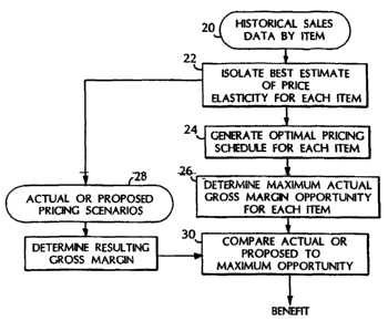
Figure 1 is a flow chart.
Figures 2 and 3 are graphs.
Figure 4 is a price elasticity chart.
Figure S is a histogram of gross margin percentages.
Figure 6 is a flow chart.
Figure 7 is a block diagram.
One goal in measuring the success of markdown management is to
define a consistent method to compare the opportunities for
improved margin across different items. The performance of
markdown management is often measured by considering the total
gross margin dollars for a group of items generated by one
markdown management system against the total gross margin
dollars generated for the group of items by another markdown
management system. Such a performance measurement forces one
to inherit the maximum gross margin opportunities defined by the
merchandising decisions for each item from a predetermined
inventory commitment and an initial pricing value for that item. A
fairer measurement of markdown management would measure
performance of each item against an intrinsic maximum
opportunity available for that item, rather than measuring the
4
CA 02488197 2004-11-30
WO 03/105053 PCT/US03/17803
aggregated total gross margin dollars from one system to other
system (or one year to another year) for a group of items.
As shown in figure 1, one way to establish an intrinsic maximum
gross margin opportunity (by maximum gross margin opportunity,
we mean the limit that you cannot exceed with perfect knowledge;
and by optimal gross margin, we mean the best actual solution that
you can generate using a given marledown system) for an item is
to analyze historical information about sales of different items 20
to isolate a best estimate of the price elasticity for each item 22.
Once the best estimate of an item's price elasticity is obtained, the
optimal pricing schedule (e.g., markdown scenario) for the item is
generated 24 by searching for an optimal gross margin for the item
26.
Once this optimal gross margin for an item is determined,
historical or proposed in-season pricing schedules 28 can be
determined using the price elasticity estimate and can be compared
against the maximum opportunity available for that item 30.
By an optimal markdown scenario, we mean the timing and depth
of a series of markdowns that provide the maximum (theoretical)
gross margin for an item by the end of the selling period (e.g., the
end of a season).
Within the boundary conditions of an initial inventory amount and
an initial retail price, the goal is to maximize the available gross
margin opportunity by finding an optimal markdown scenario.
Note that, if the initial inventory decision were perfect such that
the full inventory would be sold during the season at the full retail
5
CA 02488197 2004-11-30
WO 03/105053 PCT/US03/17803
price, there would be no reason to take any markdown; in fact,
every markdown scenario would hurt the total margin for the item.
On the other hand, if a retailer had more inventory than could be
sold at the full initial retail price, different markdown scenarios
would produce different gross margin results. Therefore, the
absolute maximum gross margin of an item depends on the initial
inventory and the full retail price, and markdown scenarios will
determine how closely one can reach the maximum gross margin
opportunity for scenarios that fall within the boundary conditions.
For a given retail merchandise item of commerce having an initial
inventory Io and an initial full price po, the gross margin function
is:
le
GM(Io~ho)= ~P(t)~'(1>>t)dt+p5(Io-Se)-clo~ (1)
Io
where p(t) is the pricing schedule, S(p, t) is the consumer demand
sales rate as a function of price p and time t, ps is the salvage
price per unit of the inventory that is unsold at the end of the
selling period, Se is the units sold between start time to and the
outdate (end of selling period) to , and c is the cost per unit of the
item. Thus, gross margin depends on the pricing schedule, and
when the pricing schedule is optimal, the maximum possible gross
margin GM~ can be achieved. Because the gross margin GM
generated by each different pricing schedule for a given item can
be meaningfully compared with other merchandise items only
6
CA 02488197 2004-11-30
WO 03/105053 PCT/US03/17803
relative to the maximum gross margin opportunity GM* , we
renormalize the definition of the gross margin GM as:
GM = AGM * GM) .
GM* ~2)
The opportunity of a given pricing schedule can thus be thought of
in terms of this normalized gross margin GM or a normalized
gross margin percent which represents the percentage deviation
from the optimal gross margin.
Because gross margin also depends on the sales rate as a function
of time and price, that is on the consumer demand, we generate a
good measurement of a key factor of consumer demand: price
elasticity. By price elasticity we mean the sensitivity of the change
in demand that is occasioned by a change in price. Using price-
elasticity of an item, one can not only estimate the true maximum
gross margin opportunity associated with each retail merchandise
1 S item, but can also simulate meaningful likely gross margin
outcomes for different markdown scenarios. This yields a rigorous
way to evaluate the results of different markdown scenarios in an
"apple-to-apple" comparison. For each item of a set of items f
commerce, a given markdown scenario will produce a value of
normalized gross margin that represents the percentage by which
the gross margin produced by the scenario falls short of a
maximum gross margin for that item. A probability distribution
can be expressed for the normalized gross margin percentages for
all of the items under consideration. A different markdown
scenario applied to all of the items will produce a different
7
CA 02488197 2004-11-30
WO 03/105053 PCT/US03/17803
probability distribution of normalized gross margin percentages.
The merits of the two different markdown scenarios can be
compared by analyzing the two probability distributions.
As mentioned with respect to figure 1, an item's price elasticity
can be estimated 22 by analyzing historic sales data 20.. Once the
item's elasticity is determined, a postseason (after-the-fact) optimal
markdown scenario can be determined 24.
Measuring the absolute maximum gross margin GM* of an item
26 would require perfect knowledge of consumer demand and
price elasticity. In the absence of perfect knowledge, we use, as
much information as possible to make a best estimation of the
demand components and price elasticity.
As a base model to represent demand for an item, we use a causal
demand model in which the overall demand is decomposed into
several causal factors: seasonality, intrinsic product life cycle,
inventory effect, and price elasticity. We express the sales rate
function as:
S(p,t) = SI(t~,)PLC(t)R(p)f (I) (3)
where SI (ty ) is a time dependent function that expresses the
seasonality of demand (bathing suits are in higher demand in May
than in September, for example).
_ z
PLC(t) = N (t - to ) exp - (t 2t Zo ) + C (4)
pk
CA 02488197 2004-11-30
WO 03/105053 PCT/US03/17803
is the product life cycle function (fashion shoes have a peals of
demand shortly after sales begin, and the demand trails off over
time) where N is a normalization parameter, t pk is a model
parameter represents the peak time of the product life cycle
function, and C a constant baseline offset model parameters
(define).
R(p) is the a price elasticity function and is defined in equation 8
below, and the inventory effect function is
I
f(I) = I~ ° I < I~ ~ (
l, I >_ I
for
r
I(t) =Io - ,~s(P~t)dt,
ro
where I(t) is the inventory at time t, the initial inventory is Ip , and
the critical inventory level I~ . is a model parameter, below this
number the overall demand goes down by the factor in equation 5
and above this number has no effect. The inventory effect function
expresses the notion that sales are adversely affected when the
inventory falls below a critical level.
Price elasticity is a key factor in markdown management. The fact
that demand changes in response to a markdown (called a
9
CA 02488197 2004-11-30
WO 03/105053 PCT/US03/17803
markdown effect) is a fundamental dynamic principle of
markdown management. Therefore, it is important to separate the
markdown effect from other components of the demand function.
We use a separable multiplicative time-independent price elasticity
model. Empirical evidence indicates that using a separable
multiplicative approach has no significant flaw. Empirical
evidence also indicates that using a time-independent formulation
is justified. That formulation is also supported by the fact that we
are focusing on short-life-cycle items. We express our general
demand function as:
S(P~ t) = R(P)B(t~ Po )a (~)
where the non-time-dependent price elasticity term is
P (g)
R(P~ Po) _
Po
for a current price p, a full retail price po, and a price elasticity
parameter y, and where the time dependent factors are expressed in
a single base demand term:
B(t;po), which is the base demand at the full retail price po as a
function of time t.
We want to determine the best estimate of base demand and price
elasticity. To do this, we fit the demand model to postseason (after
the fact) sales data to make the best estimation of the underlying
model parameters. Expressing the sales function using a main
CA 02488197 2004-11-30
WO 03/105053 PCT/US03/17803
variable separation between the base demand and price elasticity
makes our approach powerful. Determining the best estimation of
the price elasticity function as a multiplicative factor independent
of the base (time-dependent) demand model permits adjusting
actual sales units in light of any pricing decision independent of
the base demand factor.
The postseason optimal pricing schedule is intended to represent
the best pricing schedule possible given the client's business rules
and observed week-by-week sales for the item. Examples of
business rules include "no markdown until 4 weeks after item
introduction" and "subsequent markdown interval should be
separated by at least 2 weeks". Based on the best-estimated price
elasticity function, the actual sales rates of equation 7 are
determined for different possible pricing schedules. This process
makes overall demand modeling much less critical to the
estimation of the maximum gross margin opportunity. Because the
actual price, inventory level, and unit sales for each week are
known, no assumptions about an underlying seasonality or PLC
need to be applied. Simulations of the season with different pricing
schedules need only account for the different prices and inventory
levels effective each week using the demand model.
The demand model may be summarized in a single equation,
which attempts to capture the effect on demand of changes in price
and inventory level, relative to their historical values and
independent of all other factors. Relative to the observed price p
and inventory level I , the new price p' affects demand through
11
CA 02488197 2004-11-30
WO 03/105053 PCT/US03/17803
the price elasticity y , and the new inventory level I' affects
demand through the inventory effect and its critical inventory level
I
~ max ~ ,1
S~ = S p ° ~ (9)
pl max ~ , l
where S is the original observed sales rate and S' is a simulated
sales rate at price p' and inventory I' . As shown in equation 9,
there is no explicit dependence on the sales rate demand model but
only to actual sales rate units.
Note that for y > 0 , as usually assumed, this implies that lower
prices will drive greater sales. Also, at inventories below the
critical inventory level, decreasing inventory will result in
decreasing sales. The basic form of both of these dependencies has
been verified by fitting product life cycle data (PLC) to sales data
of individual items for many retailers. In any given case, the values
of y and I~ will be determined, from a postseason fit to the sales
data and should be reliable. Thus, as long as the relative changes in
price and inventory level are not too severe, equation 9 should
provide a good estimate of the sales that would have been realized
under a new markdown scenario. In particular, no assumptions
about item seasonality or an underlying PLC need to be made:
As shown in figure 6, in an actual simulation, the actual sales rates
80 are adjusted 82 only by equation 9 and actual business rules 84
12
CA 02488197 2004-11-30
WO 03/105053 PCT/US03/17803
are applied to search 86 for an optimal markdown scenario using,
for example, either a genetic algorithm or exhaustive search
algorithm. In addition to allowing a good postseason estimate of an
optimal markdown scenario for an item, this technique of adjusting
sales week by week to reflect changes in price and inventory also
represents a good method for evaluating alternative proposed
markdown scenarios against one another and against actual history.
The procedure is used with equation 9 applied to the historical data
and to the new pricing schedule, week by week, to calculate the
new sales history and cumulative gross margin.
An ultimate goal is to perform in-season simulation of markdown
scenarios while the season is in progress. For each week of a
simulated season, the simulation software will be applied to make
a fit to historical data and determine a new price. The new price
will be implemented and the sales history adjusted by equation 9.
At the end of the season, outdate salvage values will be evaluated
for the remaining inventory and the total gross margin will be
calculated. In the weekly simulation process, there are two price
elasticity functions. The best price elasticity parameter estimated
from the postseason model fit is used to apply sales rate adjustment
according to equation 9; while, as an in-season simulation is
occurring, a limited weekly data sample is used to make the best
estimation of the demand model parameters including the in-
season price elasticity estimation.
Empirical results have obtained from using an actual specialty
retailer's data to perform two components of data analysis and
13
CA 02488197 2004-11-30
WO 03/105053 PCT/US03/17803
simulation: analytic model fit and post-season optimal markdown
scenario measurement.
Examples of the baseline demand model (equations 3-8) as fit to
actual data from a retailer are shown in figures 2 and 3. The
S example of figure 2 shows data from one specialty retailer and
figure 3 shows data from another specialty retailer. (Both retailers
sell women's merchandise). The overall baseline demand model is
represented by solid black lines 38 and the actual sales unit data 40
are represented by blue starred lines. By analyzing the difference
between these two lines, one can see how good the model fits the
actual data. We use least-square minimization based on the chi-
square statistics for fitting. The search algorithm is the genetic
algorithm.
Finding a way to obtain an accurate measurement of price
elasticity is a key objective of the model fitting process. As shown
in figures 2 and 3, a typical pricing schedule 42 is essentially a
series of steps. The most sensitive price elasticity information is
embedded in the boundaries of the price steps (please define what
you mean by boundaries of the price steps (e.g., significant price
changes week to week) ). Our fitting algorithm takes advantage of
this insight by weighting the effects of bigger week-to-week price
changes more heavily relative to the full price more heavily. This
weighting consistently causes the model to better follow the sales
demand change from the markdown effect.
A summary plot of price elasticity estimated from model fittings
with historic data for 150 items is shown in figure 4. The plot
14
CA 02488197 2004-11-30
WO 03/105053 PCT/US03/17803
shows a reasonable distribution with most items falling between
price elasticity parameters (gamma) of 1.0 to 2.5. Figure 5 shows
the number density distribution of percent gross margin differences
between post-season optimal simulation results and actual historic
data for 150 items normalized by the optimal results for the 150
items. This plot shows that there is room to improve gross margin
of these items by 11 % on average.
The techniques described above can be implemented in software or
hardware or a combination of them. For example, as shown in
figure 7, the historical sales data may be stored on a mass: storage
medium 90 for use by a server 92. The server includes a
microprocessor 94 controlled by system software 96 and
markdown software 98 stored in memory 100. The markdown
software performs all of the functions described above including
the best estimation of price elasticity and the optimization
processes.
Although some examples have been discussed above, other
implementations are also within the scope of the following claims.