Note: Descriptions are shown in the official language in which they were submitted.
CA 02611748 2007-11-27
WO 2006/125274 PCT/AU2006/000706
SYSTEM AND METHOD FOR RISK ASSESSMENT AND PRESENTMENT
CROSS REFERENCE TO RELATED APPLICATIONS
[0001] The present application claims priority to Australian Patent
Application No.
2005902734 filed on May 27, 2005, and entitled "Methods, Devices And A
Computer Program For
Creating Information For Use In Facilitating A Risk Assessment," which is
incorporated herein by
reference in its entirety.
BACKGROUND
[0002] Risk is inherent in every type of business and commercial activity.
Heretofore, systems and methods have been developed to calculate, measure, and
manage risk. Such
systems and methods have included assigning loss probability distributions to
risks associated with
processes employed by an organization. These loss probability distributions
are intended to better
assess and predict risks.
[0003] By way of example, U.S. Patent Application Publication No. 2003/0149657
entitled "System and Method for Measuring and Managing Operational Risk,"
describes assigning a
loss probability distribution to a risk. In Paragraph [0042], it describes a
loss event that can be
modeled as a frequency or severity distribution. As another example, U.S.
Patent Application
Publication No. 2003/0236741 entitled "Method for Calculating Loss on
Business, Loss Calculating
Program, and Loss Calculating Device," describes business-specific loss
probability distributions. It
provides an example in Paragraphs [0075] - [0079] of a loss probability
distribution in the loan
business.
SUIVIMARY
[0004] Described herein are exemplary embodiments that present an integrated,
hierarchical process view of business operations and associated operational
and compliance risks and
controls. The presentation hierarchy shows the relationship between summary
level process maps
and the underlying detailed level process maps. The hierarchy contains risk
and control attributes
associated with any particular process. Process attributes in the hierarchy
link bottom level
processes to the individual business line, department, product, customer
segment, or any other
aspects of a business operation.
1
SUBSTITUTE SHEET (RULE 26) RO/AU
CA 02611748 2007-11-27
WO 2006/125274 PCT/AU2006/000706
[0005] The exemplary embodiments enable the estimation of a probability
distribution of possible losses arising from the failure of business
processes. The loss probability
distributions of bottom level processes can be aggregated according to
respective attribute
hierarchies, providing a more integrated and summary view of operational risk
and control
effectiveness. The hierarchy allows for the examination of specific processes
for their risk and
compliance relevance and improvement needs. The risk implications of changes
within an
organization can be assessed due to the linking of process change and
operational risk. Control
effectiveness, process value at risk, and a comparison of self-assessment
against independent
assessment can also be measured.
[0006] Currently, it is contemplated that the exemplary embodiments can be
implemented using a computer program product that receives multiple
parameters, can cross
correlate these parameters, and present parameters within a framework having
attributes
corresponding to an organization.
[0007] The methodology described herein is applicable to all industry sectors
but it is
worth noting one particular application within the financial services
industry. In the financial
services industry, the Basel II operational risk compliance guidelines require
various levels of
operational risk measurement sophistication depending on the size and
complexity of the financial
services operations. The most sophisticated guidelines are referred to as the
advanced measurement
approach (AMA). The particular bottom up approach of the exemplary embodiments
is likely to
inform and interact with AMA operational risk quantification methods to
provide additional insight
into operational risk behavior.
[0008] The exemplary embodiments can use the Basel II definition of
operational
risk, which states that "Operational risk is defined as the risk of loss
resulting from inadequate or
failed internal processes, people and systems or from external everits."
Alternatively, this definition
could be changed to exclude losses arising from external events so that only
those risk events arising
from within the organisation are considered.
[0009] Another area where the exemplary embodiments can provide input and
complement AMA methods is its capacity to isolate the contribution of
regulatory coinpliance risk to
operational risk. For example, the Sarbanes Oxley Act of 2002 (SOX), is
effectively a prescription
2
SUBSTITUTE SHEET (RULE 26) RO/AU
CA 02611748 2007-11-27
WO 2006/125274 PCT/AU2006/000706
for a set of controls that manages a category of operational risk. The
operational risk that SOX seeks
to manage is the risk of misrepresenting the underlying assets and liabilities
of the organization in
the financial reports. The exemplary embodiments can provide a detailed
insight into the process,
risk and control issues associated with compliance risk in general and
therefore enable organizations
to manage it more effectively.
[0010] Another application of the exemplary embodiments is information
technology
(IT) infrastructure integration, process standardization, centralized
controls, event management and
other operational risk management benefits. There is a large risk exposure in
IT infrastructure
support business processes and the failure of these systems. One such risk is
the management of
numerous disparate IT systems. The lack of a centralized data base or
mechanism to co-ordinate
their management is costly, complex and represents considerable operational
risk to the business.
The exemplary embodiments described herein enable the measurement of
operational risk exposure,
which can be used to justify the introduction of solutions based on cost and
operational risk
behaviour.
BRiEF DESCRIPTION OF DRAWINGS
[0011] Figure 1 is a general diagram of a risk assessment and presentment
system in
accordance with an exemplary embodiment.
[0012] Figure 2 is a hierarchy presentation of process levels generated by a
software
application in the exemplary system of Figure 1.
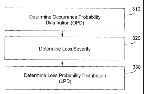
[0013] Figure 3 is a flow diagram depicting operations performed in the
exemplary
system of Figure 1.
[0014] Figure 4 is a flow diagram depicting operations performed to determine
probability of an event and an amount of event balance based on different
frequency levels and
severity intervals in the exemplary system of Figure 1.
[0015] Figure 5 is a tree diagram depicting different possible event
conditions.
3
SUBSTITUTE SHEET (RULE 26) RO/AU
CA 02611748 2007-11-27
WO 2006/125274 PCT/AU2006/000706
[0016] Figure 6 is a tree diagram depicting different possible event
conditions where
the worst event is one of a yearly event.
[0017] Figure 7 is a flow diagranl of operations performed in an inter-process
aggregation technique used in the system of Figure 1.
[0018] Figure 8 is a flow diagram depicting operations performed in a
likelihood
distribution method.
[0019] Figure 9 is an organizational schematic depicting an exemplary
embodiment
implemented into an organizational setting.
[0020] Figure 10 is a cross function process map for a credit default swap
process
[0021] Figure 11 is a parent child process map hierarchy for a credit default
swap
process
[0022] Figure 12 is a parent child process hierarchy for a credit default swap
process
showing a top to bottom orientation.
[0023] Figure 13 is a parent child process hierarchy for a credit default swap
process
showing a left to right orientation.
[0024] Figure 14 is a screen display of an interface of a software application
with
functionality for constructing a parent child process hierarchy.
[0025] Figure 15 is a number different comptuer interfaces containing a
variety of
different hierarchies.
[0026] Figure 16 is a display depicting intra-aggregation of two risks for the
selection
valuation model process.
[0027] Figure 17 is a display depicting inter-aggregation of risks for all
child
processes associated witli a trade assessment process.
4
SUBSTITUTE SHEET (RULE 26) RO/AU
CA 02611748 2007-11-27
WO 2006/125274 PCT/AU2006/000706
[0028] Figure 18 is a display depicting intra-aggregation of all intertial
fraud risks
associated with credit default swap processes.
DETAILED DESCRIPTION OF EXEMPLARY EMBODIMENTS
[0029] Figure 1 illustrates an exemplary risk assessment and presentment
system 100.
The system 100 includes a computer 102 and a database 104. The system 100 also
includes a
networlc 106 to which the computer 102 and database 104 are connected. The
computer 102 has
software including an operating system that provides various system-level
operations and provides
an environment for executing application software. In this regard, the
computer 102 is loaded with a
software application that provides information for use in facilitating a risk
assessment. The database
104 stores data that is used by the computer 102 in creating the information
for use in facilitating the
risk assessment.
[0030] The software application on computer 102 allows a user to identify
various
processes performed by an organization. For instance, the user could identify
that the organization
performs a credit check process on all new clients. The software application
allows the user to
arrange the various identified processes into a tree-like structure or
hierarchy 200, which is
illustrated in Figure 2.
[0031] Each of the nodes in the hierarchy 200 represents the various processes
identified by the user. The hierarchy 200 illustrates the relationship
(child/parent) between the
various processes performed by the organization. It is noted that the software
application can store
the identified processes according to the hierarchy 200. The software
application is such that it
provides a graphical user interface (GUI) that enables a user to identify the
processes and arrange
them in to the hierarchy 200.
[0032] According to an exemplary embodiment, the user constructs the hierarchy
200
utilizing a standard hierarchy from a library. Alternatively, a hierarchy
creation tool can be used,
such as the Corporate Modeler computer software available from Casewise
Systems and described
on the Internet at www.casewise.com.
SUBSTITUTE SHEET (RULE 26) RO/AU
CA 02611748 2007-11-27
WO 2006/125274 PCT/AU2006/000706
[0033] There are numerous ways to represent a process in graphical form. For
example, a credit default swap process which typically occurs in a financial
service institution could
be documented as a: cross functional process map (see Figure 11); a parent
child process map
hierarchy (see Figure 12); a parent child process hierarchy with a top to
bottom orientation (see
Figure 13); a parent child process hierarchy with a left to right orientation
(see Figure 14). All of
these representations and numerous other possible process docuinentation
conventions can be used
to convey important process information for various management purposes, such
as, documentation,
resource allocation, control, perfonnance measurement and so on. The choice of
representation is
dependant on management's specific requirements. The exemplary embodiments are
not dependant
on one process representation. For example, the credit default swap examples
described with
reference to Figures 12-14 demonstrates how the parent child process
relationships could be
established. As such, there is flexibility in utilizing third party process
mapping software to create
the parent child process hierarchy. But if third party software is not
available, then the parent child
process hierarchy can be established using software with functionality similar
to that described with
reference to Figures 14-18. The construction of the process hierarchy can be
achieved through'
importing process data from other programs or constructed by nominating the
various child
processes as defined by the business and attaching these to the relevant
parent processes, also
defined by the business, via the add and delete funetion.
[0034] An advantage of allowing the processes to be arranged into the
hierarchy 200
is that it can be used to reflect the decision making structure of the
organization. Processes are
represented by nodes 202, 204, 206, and 208. For example, nodes 204 represent
the "level 1"
processes which can be those processes relevant to upper management while
nodes 206 represent the
"level 2" processes which can be those processes relevant to middle
management. Nodes 208
represent the bottom level processes which are identified to a granular level
and granted additional
attributes such as "process owner/manager," "business line," "department/cost
center," "product,"
and so on. Further attributes such as "branch," "sales channel," etc. can be
added to the list so far as
they are of interest to management for reporting purpose. The hierarchy 200
allows for "process
costs," "operational risks," and "control measures" to be attached to bottom
level processes.
Overall, this "tagging system" facilitates the generation of tailored
management reports for any set
or combination of process attributes. It should also be noted that any number
of process attributes
such as those previously described, except for risks and controls, can be
attached to parent processes.
6
SUBSTITUTE SHEET (RULE 26) RO/AU
CA 02611748 2007-11-27
WO 2006/125274 PCT/AU2006/000706
[0035] In addition to allowing the user to identify the various processes
perforined by
the organization and arrange those processes in to the hierarchy 200, the
software application loaded
on the personal computer 102 allows the user to identify one or more risks
associated with each of
the processes identified in the hierarchy 200 and assign to each of those
risks several loss probability
distributions (which can be either discrete or continuous distributions). In
this regard, the risk might
be, for example, that a credit check performed on new clients of the
organization may in some
instances be flawed. As with the hierarchy 200, the graphical user interface
(GUI) provided by the
software application is arranged to allow the user to specify the risks.
[0036] Example loss probability distributions assigned to the risks associated
with
each process can be identified as LPD[l], LPD[2] and LPD[3]. Additional loss
probability
distributions may be used in alternative embodiments. LDP[1] represents the
probability of a loss
occurring as a result of the associated risk without the application of any
mechanisms for controlling
the risk. In the context of the exemplary embodiments, "without risk control
mechanisms" can mean
"no controls" or "minimum controls" as defined by management, depending on the
circumstances
and the preferred treatment of the respective management. Generally, the
process owner and an
independent appraiser should agree on the LPD[1]. The LPD[1] is a baseline
where control
effectiveness is measured. LPD[2] represents the probability of a loss
occurring as a result of the
associated risk when the party responsible for the process applies a technique
for controlling the risk.
The difference between LPD[2] and LPD[1] in the Expected Loss (EL) or Value-at-
Risk (VaR) with
x% confidence level pertaining to that risk, is a measure of control
effectiveness expressed in $
terms set by the process owner. LPD[3] represents the probability of a loss
occurring as a result of
the associated risk when an independent party assesses the technique for
controlling the risk. The
difference between LPD[3] and LPD[1] is the Expected Loss (EL) or Value-at-
Risk (VaR) with x%
confidence level pertaining to that risk, is a measure of control
effectiveness expressed in $ terms set
by the independent appraiser.
[0037] In order to establish the three loss probability distributions (LPD[1],
LPD[2]
and LPD[3]), the software application loaded on the personal computer 102 is
arranged to perform
various operations. Figure 3 illustrates exemplary operations performed to
establish loss probability
distributions. Additional, fewer, or different operations may be performed
depending on the
embodiment. In an operation 310, an occurrence probability distribution or the
likelihood of an
7
SUBSTITUTE SHEET (RULE 26) RO/AU
CA 02611748 2007-11-27
WO 2006/125274 PCT/AU2006/000706
event is determined. This determination can be made using historical data or,
in the absence of such
data, using estimations. In an operation 320, a loss severity or the impact of
the event is determined.
Loss severity can be quantified using a range of loss possibilities. In an
operation 330, a loss
probability distribution is determined for the predicted event.
[0038] In the situations where loss event data is available to estimate loss
probability
distribution, the following exemplary method can be used. While such data may
not be available,
the exemplary method provides a framework for a set of related questions which
can guide assessors
in the frequency and severity estimates of loss events. Such questions would
be useful when
assessors have limited access to empirical data. Instead, assessors can
generate estimates using
proxy data, qualitative data (e.g., expert opinion), or any combination of
proxy and qualitative data.
The estimates can then be supported by justifications established from answers
to the questions and
recorded for future reference.
[0039] Advantageously, the exemplary method requires assessors to scrutinize
underlying assumptions. Questions relating to frequency and severity
distributions are separately
identified, allowing assessors to scrutinize underlying components from the
loss probability
distribution. Expected loss and other statistical variables can be derived
from these components, as
well. Conventional methods, such as the Impact-Likelihood method assumes
assessors can
estimated an expected loss for a risk without analyzing the risk's underlying
loss probability
distribution aiid respective frequency and severity distributions.
[0040] Figure 4 illustrates operations performed in an exemplary loss
probability
distribution estimation method. Additional, fewer, or different operations may
be performed
depending on the embodiment. Further, it may be the case that certain
operations can be performed
in a different order. For purposes of illustration, the variable Y is the
number of years for which
historical data is considered. Assuming y years have no risk event, the
probability of risk event
occurring and not occurring (excluding worst case) are denoted by Po and P, .
That is,
PO = ylY
and
P, =1-Po
8
SUBSTITUTE SHEET (RULE 26) RO/AU
CA 02611748 2007-11-27
WO 2006/125274 PCT/AU2006/000706
[0041] The number of years with at least one occurrence of a non-zero balance
event
is n = (Y - y) . These years are arranged in ascending order of frequency of
non-zero balance event.
Each balance associates to a value of gain or loss. The respective sequences
of year and its
corresponding sequence of frequency of non-zero balance event are represented
as follows:
yl'y21. yn
and
f(1) I f(2), . . . f(n)
The variables f(l) and f(õ) are the respective minimum and maximum frequencies
of the above non-
zero balance event sequence. The frequency range is divided into three equal
sub-intervals. The
length of the sub-interval is:
l f = (f(õ) - f(,))/3
The variables fx and fy are the two points that equally divide the interval
f(õ) ]. As such,
.
fx = f(,) + l f and fy = f(,) + 21f
[0042] In an operation 410, frequency class intervals are defined as Low
Frequency,
Medium Frequency and High Frequency. The Low Frequency Class has the range
from f(,) to fX .
The Medium Frequency Class has a frequency value greater than fX and less than
or equal to fy
while the Higll Frequency Class has a frequency value greater than fy and less
than or equal to f(õ)
NL, Nm, and NH are the numbers in each respective Low, Medium and High
Frequency Class. It
should be noted that: NL + Njf + NH = n.
[0043] PNL , PNA1 and P,,N represent the probability of a low, medium and high
level
of event occurrence (excluding worst case and no event), respectively. They
are defined as:
PNL = NLl n, PNM = Nml n and PNH = NH l n.
The variable p is be the total number of non-zero balance event within those n
years. As such,
9
SUBSTITUTE SHEET (RULE 26) RO/AU
CA 02611748 2007-11-27
WO 2006/125274 PCT/AU2006/000706
In an operation 420, non-zero balance events are arranged in descending order
of their balance. The
sequence of the event balances is: b(,) , b(z), ... , b(p) . The variables b0)
and b(p) are the respective
maximum and minimum balance of the above sequence of balances. The balance
range is divided
into three equal sub-intervals. The length of the sub-interval is: lb =(b(l) -
b(p)) / 3. The two points
that equally divide the interval [ b(l) , b(p) ] are bx and by . Hence, bx =
b(1) - l6 and b y= b(,) - 21b .
[0044] In an operation 430, severity class intervals are defined as Low
Severity,
Medium Severity and High Severity. The Low Severity Class has a range from
b(l) to bx . The
Medium Severity Class has a balance value greater than bx and less than or
equal to by while the
High Severity Class has a balance value greater than by and less than or equal
to b(p) . Each b(;) falls
into one of the severity classes and it also associates to a particular year.
Depending on the
frequency of event occurrence of that year being considered, b(;) belongs to
the corresponding
Frequency class. Table 1 shows a three by three Table of Frequency Occurrence
Class and Severity
of balance incurred. If the number of b(;) in each cell is counted, each
syinbol in Table 1 represents
the total count of a particular cell. If all the b(;) 's value in each cell
are added, each symbol in Table
2 shows the total balance of a particular cell.
Table 1
Frequency Severity Total
Low Medium High
Low nLL n,11 nLH NL
Medium nAqL n,. nMH NM
High nxL nHM nHx Nx
Table 2
Frequency Severity Total
Low Medium High
Low ALL 14cu AcH AL
Medium AML AMW AMy AM
High AHL AHM AHH Ax
SUBSTITUTE SHEET (RULE 26) RO/AU
CA 02611748 2007-11-27
WO 2006/125274 PCT/AU2006/000706
[0045] The worst case scenario happens every t years. The worst case of loss
amount is denoted as T. It is assumed that the worst case scenario is
independent to the yearly
event. Figure 5 shows different possible event conditions. In an operation
440, the probability of an
event is determined, in an operation 450, the amount of event balance is
determined. The probability
of getting a different event condition is shown in Table 3 witli the
corresponding ainount of event
balance. Figure 6 illustrates different event conditions where the worst event
is part of a yearly
event.
Table 3
Event Probability of Event Amount of Event Balance
Worst Case and no event (1 / t) x Po T
occurrence
Worst case, non-zero (1 / t) x Pi x PNL T + AL
balance events and low
frequency occurrence
Worst case, non-zero (1 / t) x Pl x PNM T + AM
balance events and medium
frequency occurrence
Worst case, non-zero (1 / t) x P, x P,H T + AH
balance events and high
frequency occurrence
No worst case and no event (1-1 / t) x P. 0
occurrence
No worst case, non-zero (1-1 / t) x P, x Pn,L AL
balance event and low
frequency occurrence
No worst case, non-zero (1-1 / t) x Pi x PNM AM
balance events and medium
frequency occurrence
No worst case, non-zero (1-1 / t) x P, x PNX AH
balance events and high
frequency occurrence
[0046] Once the software application on the computer 102 has calculated the
loss
probability, the software application can provide information for facilitating
a risk assessment. In
this regard, the software application is arranged to allow the user to select
one or more of the
processes represented in the hierarchy 200 (see Figure 2) via a graphical user
interface (GUI).
11
SUBSTITUTE SHEET (RULE 26) RO/AU
CA 02611748 2007-11-27
WO 2006/125274 PCT/AU2006/000706
[0047] On determining which of the nodes in the hierarchy 200 have been
selected by
the user, the software application uses the selection to calculate a resultant
loss probability
distribution, which represents the information for facilitating a risk
assessment. In this regard, the
software application is arranged to perform at least two aggregating
operations on the loss
probability distributions associated with the risks associated with the nodes
in the hierarchy 200.
[0048] A first of the aggregating operations is an 'inter-process' aggregation
which
involves aggregating all the loss probability distributions that are
associated with the child nodes of a
particular node (process) in the hierarchy 200. For example, with reference to
Figure 7, the inter-
process aggregation involves aggregating the loss probabilities associated
with R; for processes P,,
Py, and PZ, Rf11 for processes Px and Py, etc. Thus, the resultant loss
probability distribution for
business unit Ba would be the aggregate of the loss probabilities associated
with RI for Px, Py, and PZ,
the aggregate of the loss probabilities R;;; for Px and Py, etc. Table 4 shows
example loss
distributions of R; for Px, Py and PZ to illustrate this aggregation
methodology.
Table 4
Px Py P"
Prob. $ Loss Prob. $ Loss Prob. $ Loss
0.3 10 0.9 5 0.5 10
0.4 20 0.05 10 0.5 30
0.3 30 0.03 50
0.02 100
11 1 1
Table 5 shows the loss distribution of Ri for P, using the figures from Table
4.
Table 5
Probability of loss $ Amount loss
0,135 =0.3x0.9x0.5 25=10+5+10
0.135 =0.3x0.9x0.5 45=10+5+30
0.0075 = 0.3 x 0.05 x 0.5 30=10+10+10
12
SUBSTITUTE SHEET (RULE 26) RO/AU
CA 02611748 2007-11-27
WO 2006/125274 PCT/AU2006/000706
0.0075 =0.3x0,05x0.5 50=10+10+30
0.0045 = 0.3 x 0,03 x 0.5 70 =10 + 50 + 10
0.0045 = 0.3 x 0.03 x 0.5 90 = 10 + 50 + 30
0.003 = 0.3 x 0.02 x 0.5 120 = 10 + 100 + 10
0.003 = 0.3 x 0.02 x 0.5 140 = 10 + 100 + 30
0.18 =0,4x0,9x0.5 35 =20+5+10
0.18 =0.4x0.9x0.5 55 =20+5+30
0.01 = 0.4 x 0.05 x 0.5 40=20+10+10
0.01 = 0.4 x 0.05 x 0.5 60=20+10+30
0.006 =0.4x0.03 x0.5 80 =20+50+ 10
0.006 = 0.4 x 0.03 x 0.5 100 = 20 + 50 + 30
0.004 = 0.4 x 0.02 x 0.5 130 = 20 + 100 + 10
0.004 = 0.4 x 0.02 x 0.5 150 = 20 + 100 + 30
0.135 =0.3x0.9x0.5 45 =30+5+10
0.135 =0.3 x0.9x0.5 65 =30+5+30
0.0075 = 0.3 x 0.05 x 0.5 50=30+10+10
0.0075 = 0.3 x 0.05 x 0.5 70 = 30 + 10 + 30
0.0045 =0.3 x0.03 x0.5 90 =30+50+ 10
0.0045 = 0.3 x 0.03 x 0.5 110 = 30 + 50 + 30
0.003 = 0.3 x 0.02 x 0.5 140 = 30 + 100 + 10
0.003 = 0.3 x 0.02 x 0.5 160 = 30 + 100 + 30
otal = 1
After arranging the loss amount into ascending order and adding together the
probabilities for the
same loss amounts (i.e., 45, 50, 70, 90, and 140), the loss distribution of R;
for P, becomes as shown
in Table 6.
Table 6
$ Loss amt. Prob. Cumulative Prob.
25 0.135 0.135
30 0.0075 0.1425
13
SUBSTITUTE SHEET (RULE 26) RO/AU
CA 02611748 2007-11-27
WO 2006/125274 PCT/AU2006/000706
35 0.18 0.3225
0 0,01 0.3325
0.27 0.6025
50 0.015 0.6175
55 0.18 0.7975
60 0.01 0.8075
65 0.135 0.9425
70 0.012 0.9545
80 0.006 0.9605
90 0.009 0.9695
100 0.006 0.9755
110 0.0045 0.98
120 0.003 0.983
130 0.004 0.987
140 0.006 0.993
150 0.004 0.997
160 0.003 1
1
[0049] A second of the aggregating operations is an 'intra-process'
aggregation,
which involves aggregating loss probability distributions of various risks
associated with a process.
For example, again referring to Figure 7, the intra-process aggregation
involves aggregating the loss
probabilities associated with R;, R;;, and R;;;. Thus, the resultant loss
probability distribution for
process P would be the aggregate of the loss probability distributions for RI,
R;I, and R;;;. When
aggregating loss probability distributions, the software application is
arranged to talce into account
the effect that differeiit probability distributions can have on each other.
This is achieved by
processing a correlation coefficient, which the computer 102 can obtain from
the database 104 via
the communication network 106. Once the resultant loss probability
distribution has been
calculated, the software application displays the resultant distribution on
the monitor of the computer
102, or prints on paper, so that a risk assessor can use it when considering
the impact of risk.
14
SUBSTITUTE SHEET (RULE 26) RO/AU
CA 02611748 2007-11-27
WO 2006/125274 PCT/AU2006/000706
[0050] For a set of distributions where the total number of possible
combinations
becomes unmanageable to compute, a number of alternate strategies can be used
to estimate an
aggregate distribution for expected loss. One strategy reduces the number of
outcomes in each of
the individual low level distributions prior to starting the aggregation
process. For example, where a
particular low level distribution contains five possible outcomes, then the
number can be reduced
down to a lower number of outcomes using one of the methods described below.
In this way,
wliereas we may have a set of ten low level distributions to be aggregated,
witli each distribution
starting out with five possible outcomes, we can reduce the number of
computations down from n
5~l0 = 9.765 million to n= 3~10 = 59,049 by aggregating within each of the low
level distributions
prior to starting the process of aggregating the entire set of 10
distributions.
[0051] When the distribution of a parent process is constructed, the number of
possible loss values increases. This parent process can be the child process
of another parent
process. This parent and children relationship can be propagated into many
levels. The number of
calculations involved to evaluate the loss distribution from one level to
another increases drastically.
Therefore, it is desirable to restrict the number of loss values for the
distribution at each level so that
the time to complete all the calculation for all levels within a system is
within a realistic timeframe.
A method of probability aggregation together with their expected loss values
is here described.
[0052] P(W = w, )= p; is defined as the probability from a loss distribution,
W, of a
parent process (P,, ) where i=1, 2, ===, n. Each p; corresponds to a loss
value of w; . The product of
w; and p; is the expected loss when W = w; . The largest possible in is used
such that:
in
p; _< 0.5.
7=1
[0053] Three equal intervals are obtained by sub-dividing the interval [ w, ,
wm ].
Similarly, divide the interval [ w,,, , wõ ] is divided into 3 equal sub-
intervals. The variables r and s
are the respective length of the first three sub-intervals and the remaining
three intervals. Hence,
r = (w,,, = w, ) / 3
and
5=(u'n -w,n)/3
SUBSTITUTE SHEET (RULE 26) RO/AU
CA 02611748 2007-11-27
WO 2006/125274 PCT/AU2006/000706
[0054] Wliere we7 and wb are the two points that equally divide the interval
[ w, , w,n ]. Also, w, and wd are the two points that equally divide the
interval [ w,,, , wõ ]. Hence,
wa=w,+r,
wb = wl + 2r,
W, = Wn, + s
and
Wd = wm + 2s.
[0055] A set of new probabilities are calculated by considering different
range of loss
values. Each new probability (P(U = uj) ) is the sum of probabilities from the
distribution W that
their loss values fall into a particular loss range being considered. The sum
of their corresponding
expected loss values (l; ) becomes the expected loss of this new probability
(Lj ). The new loss
probability distribution and its expected loss values are shown in Table 7.
Table 7
Probability Distribution of U Expected Loss (Lj) Loss Value (uj )
P(U=u1)=P(w, <_W_<w4) L, u,=L,IP(U=u1)
P(U=u2)=P(wa<WSwb) L2 u2=L2/P(Uu2)
P(U = u3 )= P(wb < W<_ wn, ) L3 u3 = L3 I P(U -- u3 )
P(U = U4) = P(w,,, < W S w,) L4 u4 = L4 I P(U = u4 )
P(U = u5 )= P(w, < W<_ wd ) L5 us = L5 / P(U = us )
P(U=u6)=P(wd <W <_wn) L6 u6 =L6/P(U=u6)
[0056] If a loss distribution is symmetric, w,,, can be the mid-point between
wi and
wn . However, assuming the loss distribution is positively skewed, as is
typically the case, the
selection of w,n is based on the cumulated probability closed to 0.5. Totally,
six intervals are
defined. If the number of interval is still too high, it can be reduced
further, for example to four, by
defining a mid-point between w, and w,,, and another mid-point between w,n and
w,, 16
SUBSTITUTE SHEET (RULE 26) RO/AU
CA 02611748 2007-11-27
WO 2006/125274 PCT/AU2006/000706
[0057] The nuinber of values in a distribution can also be reduced by
minimizing the
sum of squared error and/or assigning a functional form. The form is done by
computing the mean
(MO) and standard deviation (SO) of the initial distribution, defining a new
distribution with fewer
possible outcomes, systematically selecting values of these outcomes U and
computing the mean
(Sn) and standard deviation (Sn) of each new distribution for each new
combination of U. Then, the
sum of squared errors is computed as sum[(Mn - MO)~2+(Sn-SO)~2], the vector of
values U
=(ul,u2,..,un) is identified that minimize the sum of squared errors defined
above, and the initial
distribution is replaced with this vector U and the associated cumulative
probabilities. The latter
technique (assigning a functional form) involves identifying the general
functional form and the
specific values of any corresponding parameters that most closely approximates
the original discrete
distribution. This can be done for a particular discrete probability
distribution by first computing the
cumulative probability function of the distribution. This cumulative
distribution function is
compared with the relevant corresponding cumulative distribution functions of
a range of continuous
distributions to identify the most appropriate approximation. The most
appropriate continuous
distribution is selected to serve as an approximation to the original discrete
probability distribution.
The selection can be based upon either (1) correlation coeff'icieiit or (2)
minimizing the squared error
of estimation, both of these measures being computed on the basis of the
cumulative distribution
functions of the original and the approximate distributions.
[0058] A second strategy for reduciing the number of values in the
distribution
invokes the Central Limit Theorem (CLT) to facilitate the summation of each
lower level
distribution into an overall aggregate distribution. The CLT states that the
mean and variance of a
sum of random variants tends toward normality, with an aggregate mean equal to
the sum of the
means and an aggregate variance equal to the sum of the variances. This
strategy can be applied to
aggregate distributions where the range of loss severities are similar, such
that the range of possible
outcomes in any given distribution does not dominate the range of possible
outcomes in all other
distributions and where each distribution to be summed has finite mean and
variance.
[0059] Where there exists a subset of low level distributions to be
aggregated, each
member of the subset having a range of possible outcomes that are within the
same order of
magnitude, then the CLT can be invoked to estimate the moments of the
aggregated distribution.
The shape and confidence intervals for an aggregated distribution can then be
computed using the
17
SUBSTITUTE SHEET (RULE 26) RO/AU
CA 02611748 2007-11-27
WO 2006/125274 PCT/AU2006/000706
aggregate mean and variance together with a table of percentiles for the
appropriate "attractor"
distribution. In the most general case this will be the standard normal
distribution. Where there
exists more than one subset within a given set, then the CLT method can be
applied separately to
each subset to generate an aggregate distribution for each subset. Then the
method of aggregation
described in Strategy 1 above can be used to aggregate these distributions.
[0060] Yet another strategy for reducing the number of values in a
distribution
involves any combination of strategies 1 and 2 above, selected in part or
whole and in sequence so as
to produce the best possible aggregation taking into account the number and
characteristics of
distributions to be aggregated.
[0061] Figure 8 illustrates operations performed in an exemplary likelihood
distribution metliod. Additional, fewer, or different operations may be
performed depending on the
embodiment. Further, it may be the case that certain operations can be
performed in a different
order. In an operation 810, a likelihood probability distribution (LPD) is
determined with reference
to historical data, assuming existing controls. The LPD can be determined in
accordance with
operations such as those described with reference to Figures 3-4. In an
operation 820, likelihood
indicators and impact indicators are identified. The LPD with reference to
manager's expectations is
determined assuming existing controls in an operation 830. Managers are
requested to look ahead
into the next 12 months (for example) to consider whether the values of the
"likelihood indicators"
and "impact indicators" will change. Any changes and comments are recorded. An
example of this
type of analysis is presented for a reconciliation process, see Table 8 and 9.
On the basis of this new
information the operations in Figures 3-4 are revisited so that a new LPD is
determined.
18
SUBSTITUTE SHEET (RULE 26) RO/AU
CA 02611748 2007-11-27
WO 2006/125274 PCT/AU2006/000706
" ~ Table
I 8
Ir.~~ll I II I
Lx~e~r ~o ~1~1 ~ ~ I Li ~,
n~~~. .1 s I d , õ ,
., . , ,
~~õ ~~?(4m'entS...
% of staff in reconciliation
LIi team with <3 months training 10% 17% New staff to be recruited
LI2 number of items processed 1 mil 1.5 mil Expansion of business
average outstanding duration
LI3 of unreconciled items 3 days 3 days NA
amount of staff resources
assigned to perform
LI4 reconciliation task 10 FTE's 12 FTE's Plan to employ new staff
Table 9
iUla!inlyl~ p 1 I ;i11i1 Plll!I'I'~iil .;11I11'11116 9ai lu IIVIPI iti q'r ~_
: ~unil{ ?li i 6p Ry i p unYiji il, 111
ilt~yu
I~
h9ij . I ~1,J~i ~I 1., , i ILLI I~ i!~ I' I i I' ~i~pll' IIII 'II
~nl~.!~~t~~t~fli~
average $ amount of items
IIi processed 10000 10000 NA
additional handling fees,
interest or charges on
112 unreconciled items 5% 5 lo NA
[0062] In an operation 840, managers are asked to consider whether the
"likelihood
indicators" and "impact indicators" are likely to change if the controls of
the process are relaxed one
by one. This approach can be illustrated using the reconciliation process
example similar to
operation 830. In the example below (see Tables 10 and 11), the controls are
relaxed and the
managers expected cumulative changes recorded. The managers are then in a
better position to
revisit operations described with reference to Figures 3-4 witli a list of
event loss drivers that will
direct their responses to the relevant likelihood and impact questions. Hence,
the LPD assuming
without controls can be determined.
19
SUBSTITUTE SHEET (RULE 26) RO/AU
CA 02611748 2007-11-27
WO 2006/125274 PCT/AU2006/000706
Table 10
ke~lihoo~.~~~Rela~ Rela~~~ Relas Cuanul'a'~iv~'
L~Inclicators Cxpected C1 C. C, C3 clzaiigvs
Ll~ r. llefixiitioai V=ilue
% of staff in
reconciliation team with
0
LIl <3 months training 17% 17%
number of items
LIZ processed 1.5 mil 1.5 mil
average outstanding
duration of unreconciled
LI3 items 3 days 4 days 5 days 7 days 7 days
amount of staff
resources assigned to
perform reconciliation
LI4 task 12 FTE's 12
Table 11
~-- - ~
Impaet Relat Itel;i ~~ I2ela ~ CuinulatiN r
lndicaturs LYpecte~I C1 Ci; Cl, C,, C3 clian~es
(l1y) Definition Value
average $ amount of
IIl items processed 10000 10000
additional handling fees,
interest or charges on
II2 unreconciled items 5% 6% 7% 8% 8%
[0063] The operations may reveal that some controls do not impact on any of
the
likelihood impact indicators. This result may indicate one or more of the
following situations: (i) the
controls are "detective" rather than "preventative," (ii) some indicators are
not properly identified, or
(iii) the controls are redundant.
[0064] Figure 9 illustrates an exemplary process for integrating operational
and
compliance risk into risk adjusted performance metrics. Additional, fewer, or
different operations
may be performed depending on the embodiment. Further, it may be the case that
certain operations
can be performed in a different order. In an operation 910, data and
performance metrics are
defined. Such metrics can be different for different groups of an
organization. For example,
SUBSTITUTE SHEET (RULE 26) RO/AU
CA 02611748 2007-11-27
WO 2006/125274 PCT/AU2006/000706
business divisions or departments, line management, process owners, auditors,
board members,
compliance officers, and the such can define different data and performance
metrics. Process
owners can gather data, identify key risk indicators, assess risk and control,
and generate process
maps. Line management can review the process maps, review risk and control
assessment, and
identify process metrics. Other functions can be carried out by different
entities within the
organization, as appropriate.
[0065] In an operation 920, an operational risk calculation is performed. This
operational risk calculation can include the risk calculations described with
reference to the Figures
herein. The board of directors can set the operational and compliance risk
appetite and confidence
levels. Auditors can review the board's decisions and directions. In an
operation 930, there is an
allocation of operational risk capital and a calculation of risk adjusted
performance metrics (RAPM).
For example, operational risk capital can be allocated to relevant owners.
Incentives for line
managers and process owners can be set. Metrics can be calibrated and
adjustments made based on
results from the risk calculations.
[0066] In an operation 940, a variety of different reports are generated and
analysis
performed at all levels of the organization. In an operation 950, risk
adjusted productivity is
managed. For example, process owners can collect risk data and deploy
resources in accordance
with operational risk metrics and risk adjusted performance metrics
objectives. Line management
can deploy resources in accordance with these objectives and divisions or
departments can align
resources according to these objectives. In an operation 960, process
structures and/or risk profiles
are updated and the evaluation process continues.
[0067] Figure 10 illustrates a cross-function process map for a credit default
swap
process. The process map graphically illustrates operations behind a credit
default swap, including a
trade assessment, trade negotiation, and trade execution. Figure 11
illustrates a parent child process
map hierarchy for the credit default swap process. The hierarchy presents the
various component
parts that make us the credit default swap. Figure 12 illustrates a top to
bottom orientation to the
credit default swap process. Figure 13 illustrates a left-to-right orientation
to the credit default swap
process. Such a left-to-right orientation can be depicted in a computer user
interface, using
collapsible and expandable folder and sub-folder structures. An example
computer interface having
21
SUBSTITUTE SHEET (RULE 26) RO/AU
CA 02611748 2007-11-27
WO 2006/125274 PCT/AU2006/000706
the hierarchy depicting in a left-to-right orientation is shown in Figure 14.
Figure 15 illustrates a
number different comptuer interfaces containing a variety of different
hierarchies.
[0068] Figure 16 illustrates a computer interface showing inter-aggregation of
two
risks for a selection valuation model. Figure 17 illustrates a computer
interface showing intra-
aggregation of risks for all child processes associated with a trade
assessment process. Figure 18
illustrates a computer interface showing inter-aggregation of internal fraud
risks associated with
credit default swap processes.
[0069] The methodology described herein with respect to the exemplary
embodiments provides a number of advantages. For example, the exemplary
methodology attaches
operational risk attributes and loss probability distributions (LPDs) to
bottom level processes.
Operational risks; controls; budget/actual costs; and LPDs due to the
individual operational risks are
associated with the bottom level processes wliich also have attributes
including but not limited to:
owner process ID, parent process ID, process owner/manager, department to
which the process
belongs, business unit to which the process belongs, and product to which the
process is supporting.
[0070] Further, the exemplary methodology enables multiple party
evaluation/validation for the risk and control details of bottom level
processes. Process owners and
independent reviewers need to agree on the state and correctness of
operational risk and control
information prior to constructing the set of LPDs. The exemplarymethodology is
designed to
support the modeling of multiple LPDs for each operational risk at bottom
level processes to
enhance the quality of independent reviews. The use of LPDs (LPD[1]: assumed
without control
(or, as discussed above, with minimum controls defined by management); LPD[2]:
assumed with
control assessed by process owner; LPD[3]: assumed with control assessed by
independent reviewer,
...etc.) to capture multiple parties' assessment on risk and control
effectiveness enhances the
process/quality of independent review, making it more standardized, accurate,
and transparent across
the organization.
[0071] The exemplary methodology enables the inter-aggregation of the set of
LPDs
for individual risks of the bottom level processes along the respective
hierarchies of the various
attributes (e.g. process/ business unit/ department/ product/...etc.) in order
to establish a set of LPDs
for every risk at each process/ business unit/ department/ product... etc. in
their respective
22
SUBSTITUTE SHEET (RULE 26) RO/AU
CA 02611748 2007-11-27
WO 2006/125274 PCT/AU2006/000706
hierarchies. The exemplary methodology aggregates sets of LPDs (i.e, LPD[1]:
assumed without
control (or minimum control); LPD [2]: assumed with control assessed by
process owner; LPD [3]:
assumed with control assessed by independent reviewer, etc.) for individual
operational risks of the
bottom level processes to their parent processes up the process hierarchy such
that every parent
process has a corresponding set of aggregated LPDs for the respective
operational risk. This
aggregation is also performed according to the respective hierarchy of other
attributes (e.g.
individual business line, deparhnent, product,... etc). As far as their
effects are updated in the
respective LPDs and then aggregated up the respective hierarchies, changes to
the risk/control
profile at the bottom level processes are automatically reflected to all
parent processes, business
units, departments, and products.
[0072] The exemplary methodology enables the intra-aggregation of the sets of
LPDs
for all operational risks at each process/ business unit/ department/
product...etc. into 1 set of LPDs
(i.e. LPD[1], LPD[2], LPD[3]) for every process/ business unit/ department/
product ... etc. PRIM
aggregates sets of LPDs for the various operational risks under a process into
one set of LPDs for
that particular process. The same is also performed for other attributes, i.e.
individual business line,
department, product... etc. This enables the reporting of 'Expected Loss' (EL)
and 'Value at Risk
with x% of confidence level' (VaR) in dollar terms for every process/ business
unit/ department/
product.. . etc.
[0073] The exemplary methodology can provide reports quantifying the
organizations
risk capital allocation requirement. Quantitative measures of operational
risks such as 'Expected
Loss' (EL) and 'Value at Risk with x% confidence level' (VaR) are expressed in
dollar terms, and
are readily available with the LPDs for processes, departments, business
units, and products. As a
result, a basis for operational risk capital allocation is readily available
for processes, departments,
business units, and products levels using 'EL' or 'VaR' as an allocation
basis.
[0074] The exemplary methodology provides a means to identify the component of
the organizations risk capital allocation requirement that is attributed to
compliance risk. The
process, risk and control analysis prescribed by the methodology, which
includes the application of
LID, enables the aggregation of only those LPDs associated with compliance
risks. The exemplary
methodology measures control effectiveness based on LPDs and in dollar terms.
By comparing LPD
23
SUBSTITUTE SHEET (RULE 26) RO/AU
CA 02611748 2007-11-27
WO 2006/125274 PCT/AU2006/000706
'assumed with control' and LPD 'assumed without control', the methodology
enables the
measurement of control effectiveness to be based on LPDs and expressed in
dollar terms (e.g.
"Expected Loss (EL) is reduced by $n" and "Value-at-Risk with a x% confidence
level (VaR) is
reduced by $n") for individual process, business unit, department, product...
etc. Control
effectiveness measurement expressed in dollar terms facilitates the cost-
benefit analysis for controls.
[0075] The exemplary methodology recognizes the complex operational risk
behavior
that can arise from an interdependent network of business processes. Network
effect refers to the
situation where the successful performance of a process (e.g., Process A) is
dependant on the success
of another process (e.g., Process B). Therefore the failure of Process B
represents a risk to Process
A. As such, the outsourcing, for example, of Process B only removes the risks
directly associated
with it, but cannot remove the network effect that it has on Process A. The
exemplary methodology
handles this by allowing the user to specify for Process A the risk of Process
B failing.
[0076] The exemplary methodology captures correlation among different risks by
correlation factors. The correlation factors are applied when performing LPD
aggregation of the
risks involved. The exemplary methodology is not exclusively reliant on the
availability of
quantitative data. The exemplary methodology provides management with the
choice to use
quantitative or qualitative data or a blend of both to develop LPDs. In this
sense, the methodology is
not completely reliant on historical operational loss data alone.
[0077] The exemplary methodology's data capture methodology can simplify
management's task of characterizing the risk and control attributes for
processes where there is little
or no data. Processes which have a rich source of high quality data to
characterize risk and control
can be used to characterize similar processes for which there is little or no
data. In one exemplary
embodiment, an organization has already developed a robust business process
view of the
organization, where process definitions are standardized, mapped and well
documented, such that a
process hierarchy similar to the hierarchy 200 of Figure 2 is already
available or can be easily
produced.
[0078] The hierarchy 200 represents the way business processes are actually
managed
and captures the network of process relationships within the organization
i.e., how the various
processes interact. From hierarchy 200, a chart 210 is derived which is the
parent-child process
24
SUBSTITUTE SHEET (RULE 26) RO/AU
CA 02611748 2007-11-27
WO 2006/125274 PCT/AU2006/000706
hierarchy and is the basic structure defiiiing liow the various LPDs are
aggregated. The relationship
between the hierarchy 200 and chart 20 in Figure 2 can be understood by
examining the
corresponding process notation.
[0079] In a second exemplary embodiment, a business process program is not in
place. A process map hierarchy does not necessarily need to be created before
the parent-child
process hierarchy is created. Creating the parent-child process hierarchy is
not a complex exercise
because the complicated, time consuming process relationship detail is not
required. Advantage can
be gained by utilizing existing process information and any remaining gaps
quickly obtained by
requesting the input from various line managers and subject matter experts.,It
is possible to siinply
identify only the bottom level child processes perform LPD aggregations
without the parent-child
process hierarchy to place some predefined definitions to LPD aggregation.
Under this scenario the
information can still provide valuable management insiglits to operational
risk adjusted productivity,
operational risk and control behavior.
[0080] Those skilled in the art will appreciate that the invention described
lierein is
susceptible to variations and modifications other than those specifically
described. It should be
understood that the invention includes all such variations and modifications
which fall within the
spirit and scope of the invention.
SUBSTITUTE SHEET (RULE 26) RO/AU