Note: Descriptions are shown in the official language in which they were submitted.
CA 02634020 2008-05-30
SYSTEM AND METHOD FOR MULTI-LEVEL ONLINE LEARNING
FIELD OF THE INVENTION
[0001] This invention relates to a system and method for online learning,
namely
multi-level learning, which is expected to be not sensitive to the curse of
dimensionality
and have good behavior in the presence of irrelevant attributes, noise, and
even a
target function changing in time and such systems and methods are particularly
suited
to recommendation engines.
BACKGROUND OF THE INVENTION
[0002] The interactive online advertising industry is enjoying a boom in
recent
years. Everyday, thousands upon thousands of people browse e-commercial
websites
and leave without any response. The business object of a company's website is
not
merely to get more visitors, but to convert as many Web spectators into Web
participants as possible. Actually, the average response rate is only 4% for
keyword-
driven search engine advertising; most of money for advertising is wasted. A
small
improvement in response rates would be very valuable. Online recommendation
techniques are widely used to address this problem, making websites somewhat
intelligent so that the response rate can be increased. Recommender systems
are able
to influence prospective customers to commit in some way to a more substantial
relationship, e.g., purchasing products, sharing information, etc. For
example, a
recommender system, which implements online recommendation techniques, can
classify customers according to what product would resonate, and then perform
personalized recommendation by ordering options from most to least interesting
for
each customer.
[0003] People also have to deal with the challenging problem of information
overload as the amount of online data increases by leaps and bounds in non-
commercial domains, e.g., research paper searching.
[0004] Machine learning explores ways of constructing predictive models from a
given collection of empirical data. It models learning problems as searching
through a
suitable hypothesis space [5]. Typically, a greedy search strategy is required
because
CA 02634020 2008-05-30
-2-
the hypothesis space is huge [5]. Supervised learning, also known as learning
with a
teacher, is an important machine learning technique. The term "supervised"
originates
from the fact that the desired outcome of each object is provided by an
external
"teacher" [10]. Suppose we have a training dataset, in which we observe the
attribute
and outcome measurements for a set of objects. The outcomes are regarded as
the
outputs of the underlying unknown target function, given the attribute values
as inputs.
The task of supervised learning is to find a good approximation to the target
function [4].
We use the training data to build a predictive model, which will be used to
predict the
outcome for new unseen instances. There are two kinds of supervised learning
techniques: online learning and offline learning.
[0005] Although online learning is less common than offline learning, it has
attracted much attention in recent years because it is more suitable than
offline learning
in some real-world applications, e.g., real-time decision making. Sometimes,
we do not
have training data in advance, and more and more data are available after the
system is
put into use. Online learning can start with few examples and make predictions
while
learning in such situations. In many industrial applications, the data
distribution changes
gradually over time (e.g. due to wear and tear of the system). We also
occasionally
encounter an arbitrary sequence of data coming from a source that may even be
changing adversarially in response to the learning, e.g., spam emails. Online
learning is
required to learn and track time-varying functions from examples generated by
a time
dependent teacher, adapting continuously to a changing environment. In some
large
scale practical applications, the amount of data could be too huge for offline
learning
schemes to handle. Instead, online learning is employed to operate
continuously in its
environments, making predictions, receiving rewards, and suffering losses.
Online
learning is also required in processing a continuous data stream, in which
case the
learner receives new information at every moment and should adapt to it,
without having
a large memory for storing all historical data.
SUMMARY OF THE INVENTION
[0006] Online learning provides an attractive approach to online
recommendation. Online learning has the ability to take just a bit of
knowledge and use
CA 02634020 2008-05-30
-3-
it. Thus, online learning can start when few training data are available. This
is important
to a newly built recommender system, helping to alleviate the so-called cold-
start
problem. Furthermore, online learning has the ability to incrementally adapt
while we
learn more and more knowledge. Online learning comes into play when we have
repeated interactions. In each iteration, it accepts a request for prediction
of a given
example, makes a prediction, and observes the true label of the example, and
the
model is updated to improve later predictions if the observation disagrees
with
prediction [8]. Online learning can be useful for interacting with people. For
example, in
online recommendation, although the users' tastes usually remain a constant
for a long
period of time, their interests may change frequently. The present invention
allows the
user's evaluation of an object to change during the interaction and tracks
that changing
opinion. Thus, it is necessary to employ an online learning scheme to observe
their
changing ratings on objects.
[0007] In real-world applications, although binary data is sometimes used to
represented quantity, it is too coarse in most situations. Multi-level comes
into play to
predict the multi-level response from a user, for example, multi-level data is
required
when we want to predict the degree of appreciation a user may have for an
object.
Although some prototype recommender systems use binary data, that is, the
users'
ratings for items are simply classified as high (positive) and low (negative),
lots of noise
data are introduced because both missing ratings and low ratings are treated
similarly.
Actually, almost all practical recommender systems use multi-level data to
describe
users' degree of like or dislike. Typically, user ratings for items have five
levels (1 to 5),
ranging from very low to very high. Therefore, online learning with multi-
level predictions
while interacting with users is an aspect of the present invention.
[0008] The Perceptron and the Winnow are two main online learning schemes
employing linear model, which are very simple with nice properties for real-
world
applications. The Winnow scheme outperforms the Perceptron scheme in general
in
terms of convergent speed and mistake bound [8, 2]. Winnow and its variants
have
been successfully applied in many domains, such as patent document
classification and
data stream filtering [1, 2].
CA 02634020 2008-05-30
-4-
[0009] It is believed few online learning schemes have been considered in the
field of online recommendation. It is valuable to explore the applications of
the Winnow
scheme featuring very fast updates to online recommender systems.
[0010] The basic Winnow scheme and its variants can only handle binary
attributes and perform binary classification. It is necessary to extend the
Winnow
scheme to multi-level version so that it can handle multi-level attributes and
perform
multi-class classification.
[0011] The present invention relates to a multi-level online learning scheme,
called MWinnow, which is extended from the Balanced Winnow scheme. MWinnow
stands for multi-level Winnow. The MWinnow scheme is expected to be not
sensitive to
the curse of dimensionality and have good behavior in the presence of
irrelevant
attributes, noise, and even a target function changing in time.
[0012] The new MWinnow scheme is good for online recommendation because it
is very simple and cheap to implement with guaranteed real-time performance
and able
to handle many irrelevant features. Its storage requirement is negligible
compared with
offline leaning schemes because it does not need to keep any instance in
memory.
Actually, given a machine learning problem with n attributes and m classes, it
needs to
store onlym(n + 1)weights and two parameters. Also, it is not sensitive to the
curse of
dimensionality problem that is too strong for most machine learning schemes.
[0013] We systematically compared the MWinnow scheme with the baseline
scheme na'ive Bayes, by evaluating the prototype online recommender systems
adopting these schemes. The experimental results show that the MWinnow scheme
is
promising for future applications. It not only provides a practical machine
learning
approach to online recommendation, but also significantly outperforms other
schemes in
terms of both prediction accuracy and real-time performance. Furthermore,
MWinnow
can be flexibly integrated with some other machine learning scheme to improve
online
recommendation performance.
CA 02634020 2008-05-30
-5-
[0014] There are many multi-class learning problems with multi-level input
attributes. The goal is to distinguish among more than two possible classes.
For
example, a typical online recommender system has five-level scale of ratings.
It is
necessary to generalize online learning schemes to handle multi-level data,
which
means both the input attributes and class attribute are multi-level.
[0015] A computer implemented method of online learning is provided comprising
the steps of:
a. initializing all weights wj(k) in a plurality of weight vectors w(k) to a
constant a
according to the formula:
w~(k)
= a for j = 1, 2, ..., n, k = 1, 2, ..., K;
b. receiving an instance x=(xl,xZ,...,xn)", having a true label;
c. generating a predicted label Ik to classify the instance x to a class k to
according to the formula:
c(x) = lk such that k = arg max f(`) (x) ;
1Si5K
d. comparing the true label of the instance x with the predicted label Ik to
determine if a prediction is correct; and
e. if the prediction is not correct, updating the weight vectors according to
a
plurality of weight updating rules.
[0016] A computer implemented method of recommending items to a user is also
provided comprising the steps of maintaining a set of classifiers
corresponding to a set
of items for providing ratings, observing the user's online behaviour
comprising rating an
item from the set of items, updating the set of classifiers in response to an
observed
behaviour, predicting ratings for at least some of the items from the set of
items using
the set of classifiers, and recommending to the user at least one item where
the at least
one item has a high predicted rating.
[0017] Furthermore, an apparatus for recommending items to a user is provided
comprising means for maintaining a set of classifiers corresponding to a set
of items for
providing ratings, means for observing the user's online behaviour comprising
rating an
CA 02634020 2008-05-30
-6-
item from the set of items, means for updating the set of classifiers in
response to an
observed behaviour, means for predicting ratings for at least some of the
items from the
set of items using the set of classifiers, and display means for recommending
to the
user at least one item where the at least one item has a high predicted
rating.
[0018] In another aspect of the invention, a memory for storing data for
access by
an application program being executed on a data processing system is provided
comprising a database stored in memory, the database structure including
information
resident in a database used by said application program and including an items
table
stored in memory serializing a set of items, and a classifiers table stored in
memory
serializing, for each item, a predicted rating such that values in the
classifiers table may
be updated based on observing a user's online behaviour comprising rating an
item
from the set of items, and such that high values in the classifiers table
represent items
of potential interest to the user.
LIST OF FIGURES
[0019] Figure 1 is a general online learning algorithm.
[0020] Figure 2 is an illustration of the Mistake Bound Model.
[0021] Figure 3 is an example of stock market predictions.
[0022] Figure 4 is a general learning-from-expert-advice algorithm.
[0023] Figure 5 is the halving algorithm.
[0024] Figure 6 is the weighted majority algorithm.
[0025] Figure 7 is an example of weighted majority algorithm.
[0026] Figure 8 is the weighted majority algorithm (general version).
[0027] Figure 9 is the randomized weighted majority algorithm.
[0028] Figure 10 is the mistake bounds of the randomized weighted majority
algorithm.
CA 02634020 2008-05-30
-7-
[0029] Figure 11 is the hedge algorithm.
[0030] Figure 12 is the perceptron model.
[0031] Figure 13 is the perceptron algorithm.
[0032] Figure 14 are the instances separated with a margin of g.
[0033] Figure 15 is the winnow algorithm (simplified version).
[0034] Figure 16 is the balanced winnow algorithm.
[0035] Figure 17 are some commercially available recommender systems.
[0036] Figure 18 is a typical rule-based recommender system.
[0037] Figure 19 are content-based filtering recommender systems.
[0038] Figure 20 is a fragment of a user-item matrix for a movie recommender
system.
[0039] Figure 21 is a collaborative filtering recommender system.
[0040] Figure 22 is the architecture of GroupLens.
[0041] Figure 23 is the MWinnow algorithm.
[0042] Figure 24 is the design architecture of the MWinnow algorithm.
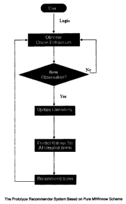
[0043] Figure 25 is the prototype recommender system based on pure MWinnow
scheme.
[0044] Figure 26 is an extraction of bell data.
[0045] Figure 27 is the confusion matrix.
[0046] Figure 28 is the k-fold cross validation.
[0047] Figure 29 are the experimental results based on binary yahoo dataset.
CA 02634020 2008-05-30
-8-
[0048] Figure 30 are the experimental results based on binary bell dataset.
[0049] Figure 31 are the experimental results based on multi-level bell
dataset.
DETAILED DESCRIPTION
[0050] Ideally, commercially viable online recommender systems collect,
cleanup,
and analyze customer intelligence data, cluster users into user sub-
populations with
similar traits where those traits are predictive of the user's selection,
purchasing and/or
consumption behaviour, collect data about each user interest, e.g., ratings
and
interactions, use predictive techniques to make recommendations, and track
changes to
the data almost in real-time so that recommendations are readily adapted to
changes in
data. It is important to look at how the community is structured, how the
individual's
interactions evolve, and how the community evolves. Moreover, people may
extraordinarily expected that the recommendations given to a customer will be
up to
date with all the information known about that customer and the associated
population,
as well as the recent activities of all other individuals in that population.
[0051] Online learning is especially useful in online recommendation. Although
users' tastes usually remain stable for a long period of time, their interests
may change
from time to time. Online learning is capable of not only making predictions
in real time
but also tracking and incrementally adapting to users' interests by observing
their
ratings on objects.
a) Overview
[0052] In online learning models, we do not assume that there is an unknown
distribution p over data, and that there are separate training and test data
sets, drawn
independently and identically distributed (i.i.d.) according to p [3]. Online
learning
schemes learn a model incrementally from data. A trial is the sequence of
events in
which the algorithm receives one example, makes a prediction on the example's
label,
and then is told the correct answer [8]. In the following discussion, we
assume that
predictions belong to the set {0, 1}, which is the special case of binary
classification.
There are many available loss functions, such as the 0-1, absolute, square,
Hellinger,
CA 02634020 2008-05-30
-9-
and entropy losses; however, in online learning schemes, we use the 0-1 loss,
which is
equal to the absolute loss with the assumption that predictions belong to the
set {0, 1).
[0053] Online learning proceeds in a sequence of trials. In each trial, the
algorithm gets an instance from some fixed domain, produces a binary
prediction based
on its knowledge of previously seen examples, receives a true label at the end
of the
trial, and calculates the loss, which may be used to perform some learning
[8]. A
general online learning algorithm is given in Figure 1 [8].
[0054] Given a set of examples(m y`V the number of cumulative
T
jL(YI,Yr,x0
mistakes is 1=1 . The goal of the learner is to make as few cumulative
mistakes
as possible. In general, the mistake bound model is used to evaluate the
performance,
that is, how many mistakes the learner makes before it learns the concept. The
definition of the mistake bound is as follows [8].
[0055] Definition Let X be the instance space and C the concept class, i.e.,
C c{ f I f : X-> 10,111. Algorithm A learns concept class C with mistake bound
M if A
makes no more than M mistakes on any sequence of examples consistent with some
fE C.
[0056] An illustration of the mistake bound model is shown in Figure 2.
Algorithm
2 makes fewer mistakes than algorithm 1 in most of the trials, thus it makes
fewer
mistakes than algorithm 1 by the end of the procedure. So algorithm 2
outperforms
algorithm 1 in terms of prediction performance. We are specifically interested
in the
worst-case mistake bound of an online learning algorithm, that is, the maximum
number
of mistakes the algorithm makes in the worst case.
[0057] There are several variants of the basic online learning model. In the
basic
online learning model proposed by Littlestone, we assume that the learner only
knows
the set of possible instances and that the sequence of instances may be chosen
by an
adversary [8]. David et al. presented a variant with a stronger assumption
that the
sequence of instances (without the labels) is known to the learner in advance
[6].
CA 02634020 2008-05-30
-10-
Goldman et al. proposed another variant called the self-directed learning
model with a
much stronger assumption [7]. In this model, the sequence of instances is
chosen
adaptively by the learner, that is, the learner chooses a new instance only
after getting
the true label of the current instance [7]. In this thesis, we only consider
the basic online
learning model.
[0058] In the online learning model, there are two kinds of uncertainties that
the
learner has to face. Firstly, like any other learning model, the target
function is
uncertain. Secondly, which instances to be presented to the learner in the
future are
also uncertain [6].
[0059] There are many practical examples of online learning problems in the
real
world, such as predicting each day whether the stock market will go up or
down,
predicting each day whether it will rain, predicting the conditional-branch
outcome in
computer architecture, filtering spam, analyzing and processing network data
streams,
finding the best candidate at a job fair when decisions must be made on the
spot,
allocating resources optimally, making sequential investments optimally, and
so on.
b) Online Learning Versus Offline Learning
[0060] Offline learning is also known as batch learning. In offline learning,
the
main assumption is that the separate training and test data sets are drawn
independently and identically distributed (i.i.d.) according to an unknown
fixed target
distribution p over data [5]. Offline learning begins with the training phase,
followed by
the testing phase. It operates on the entire data set. The goal is to gain
good
performance on the test data. The PAC model, which asks how many examples we
need to learn Probably Approximately Correctly, is used to evaluate offline
learning
schemes [5].
[0061] Online learning uses the same data to train and test at the same time,
i.e.,
making predictions continuously even while it is learning [3]. The examples
are
arbitrarily presented one by one to the learner. Learning is done
incrementally and in
real-time, with the results of learning available soon after each new example
is
acquired. The algorithms are typically very simple and fast. Online learning
schemes
CA 02634020 2008-05-30
-11-
are mistake driven. They have to decide between choosing actions to perform
well now
versus gaining knowledge to perform well later. The goal is to gain good
performance all
the time. The mistake-bound model, which asks how many mistakes we will make,
is
used to evaluate online learning schemes [3].
[0062] Online learning has several advantages over offline learning. Firstly,
online learning is potentially more robust because errors or omissions in the
training set
can be corrected during operation [3]. Secondly, it is difficult to have
training data in
advance in some situations. Training data can often be generated easily and in
great
quantities when a system is in operation, whereas it is usually scarce and
precious
before. Thirdly, the storage of the previous examples is not necessary because
only one
example is given at a time and then discarded after learning. Thus, it is much
less
memory consuming and less computationally expensive compared to offline
learning.
Fourthly, it is less susceptible to overfitting, which is a serious problem in
offline training.
Fifthly, online training has the ability to adapt to changing environments
[3]. Finally,
theoretical examinations of online learning are easier.
c) Online Learning From Expert Advice Framework
[0063] We begin with a simple intuitive problem. A learning algorithm is given
the
task each day of predicting whether it will rain that day. In order to make
this prediction,
the algorithm is given as input the advice of n experts at the start of each
trial. An expert
means anything that makes a prediction, not necessarily someone who knows
anything.
Experts can be a set of learning algorithms, people, some fixed set of
functions, a
computer model with various parameter settings, etc. Typically, experts can be
either
hypotheses within the same learning algorithm or different learning
algorithms. Each
day, each expert predicts yes or no, and then the learning algorithm (also
called master
algorithm) must use this information in order to make its own prediction. The
algorithm
is given no other input besides the yes/no bits produced by the experts. After
the
learning algorithm makes its prediction, the experts and the algorithm are
then told
whether it rained that day. Suppose we make no assumptions about the quality
or
independence of the experts, so we cannot hope to achieve any absolute level
of quality
in our predictions. In that case, a natural goal instead is to perform nearly
as well as the
CA 02634020 2008-05-30
-12-
best expert so far, that is, to guarantee that at any time, our algorithm has
not
performed much worse than whichever expert has made the fewest mistakes to
date. In
the language of competitive analysis, this is the goal of being competitive
with respect to
the best single expert.
[0064] Such a mistake driven online learning algorithm is called learning from
expert advice because it makes predictions based on the advice of experts,
where
expert advice is a (discrete or real) prediction of the outcome. By the end of
a trial, after
making a prediction, the algorithm incurs some loss that measures, via some
loss
function, the discrepancy between its prediction and the true outcome. Any
mistake
made by the master algorithm is converted into knowledge on the learning
problem.
Then a new trial starts. The general goal is to devise an expert advice
algorithm that
predicts as well as possible by utilizing experts' opinions.
[0065] For example, suppose we want to predict the stock market. We choose
four experts and use their advice somehow to make our predictions. The
predictions of
the four experts and the learner, and the outcome in each day are shown the
table of
Figure 3.
[0066] We get the totals for the number of mistakes made by the experts and
the
learner, which give us an idea of how well the learner can do. In this
example, Expert 2
is the best expert. Ideally, we would like the number of mistakes made by the
learner to
be close to that of the best expert in hindsight at the end of this sequence
of trials. The
goal is an efficient algorithm that does nearly as well as best expert. We can
restate the
procedure of a general learning-from-expert-advice algorithm formally as
follows (see
Figure 4). The goal of the learner can be represented
as M<_ m ; in m; + (small _ amount), where M is the number of cumulated
mistakes made by
the learner, and m, is the number of cumulated mistakes made by expert i, i =
1,2,...,n.
[0067] Learning-from-expert-advice algorithms has been studied extensively in
the theoretical machine learning literature [3]. A further crossover of ideas
among online
learning algorithms, computational learning theory, and game theory would be
possible.
There is evidence that expert advice algorithms have practical significance
because
CA 02634020 2008-05-30
-13-
these algorithms have exceptionally good performance in the face of irrelevant
features,
noise, or a target function changing with time.
i) Halving Algorithm
[0068] We assume that at least one expert is perfect, which always makes
decisions correctly. This algorithm maintains a list (also called version
space) of experts
that have not yet made mistakes, initially including all experts. On each
trial, the learner
makes a prediction based on a majority vote of experts in the list. This
algorithm is
described as follows (see Figure 5). The only time the algorithm makes a
mistake is
when the majority of the version space is inconsistent with the example, so
that at least
half the version space must be deleted.
[0069] We consider the mistake bound of this algorithm as follows.
Let W be the number of experts left in the version space,
and n the total number of experts.
Initially, W = n.
After making 1 mistake, W_< 2
After making 2 mistakes, W<_ 4
After making m mistakes, W< 2m
[0070] Since W _ 1, we have1 <_ W2m . Now, we get the following
inequality: m < lg n.
[0071] So the mistake bound of this algorithm is Ig n. Note that this is a
worst-
case bound. This algorithm can learn the target concept without making any
mistakes
because experts are deleted from the version space even when the majority vote
is
correct.
CA 02634020 2008-05-30
-14-
ii) Weighted Majority Algorithm
[0072] We can do nearly as well as the best expert in hindsight using this
algorithm if there is no perfect expert. The key idea is that making a mistake
does not
completely disqualify an expert. So, instead of crossing off the mistaken
experts, the
algorithm just lowers their weights. This algorithm maintains a list of
weights
w1,w2,...,wn, one for each expert, and predicts based on a weighted majority
vote of the
expert opinions. Higher weights correspond to greater importance. In each
trial, an
expert's weight (importance) is decreased if and only if the expert makes a
mistake. The
learner's prediction is a weighted majority vote by all of the experts. The
Weighted
Majority algorithm (simple version) is shown in Figure 6.
[0073] The mistake bound of this algorithm is given by the following theorem
[3].
[0074] Theorem The number of mistakes M made by the Weighted Majority
algorithm described above is no more than 2.41(m+lgn), where m is the number
of
mistakes made by the best expert so far.
[0075] An example of this algorithm is shown as follows (Figure 7). Initially,
all
four experts are assigned weight 1. After the first trial, the weight of the
fourth expert,
who made a mistake, was changed to 0.5. Two experts made mistakes in the
second
trial, and their weights were changed to 0.5.
[0076] We can extend naturally the above Weighted Majority algorithm to a more
general version. We introduce a parameter0 5P < 1. Each expert initially gets
a weight
of 1. For each incorrect prediction, we decrease the expert's weight by
multiplying it by
A. The Weighted Majority algorithm (general version) is as follows (Figure 8).
[0077] This algorithm is a generalization of the halving algorithm. If 0, we
have the halving algorithm. If P = 0.5, we have the simple version of the
Weighted
Majority algorithm. The mistake bound of this algorithm is given by the
following
theorem [52].
[0078] Theorem Given the above online learning setting, the number of mistakes
M made by the Weighted Majority algorithm described above is bounded as:
CA 02634020 2008-05-30
-15-
M<_a,=m+ca=lgn
1
lg -
where aR = 2 , cQ = 12 , and m is the number of mistakes made by the
lg 1+'6 lg 1+'8
best expert so far.
[0079] We find an interesting property of this algorithm, that is, the number
of
mistakes made depends on the performance of the best expert and the number of
experts. This algorithm is not as sensitive to noisy training data as Having,
since it never
completely eliminates any mistaken expert.
iii) Randomized Weighted Majority Algorithm
[0080] As mentioned before, the mistake bound of the Weighted Majority
algorithm (simple version) is 2.41(m+lgn), which is not acceptable if the best
expert
makes a mistake 20% of the time. We use a randomized approach to smooth out
the
worst case, which is the case in which slightly more than half of the total
weight
predicted incorrectly causes the algorithm to make a mistake and reduce the
total
weight by 4. The Randomized Weighted Majority algorithm is as follows (see
Figure 9)
[3].
[0081] The mistake bound of this algorithm is given by the following theorem
and
corollary [3].
[0082] Theorem On any sequence of trials, the expected number of mistakes M
made by the Randomized Weighted Majority algorithm described above satisfies:
min l +lnn
M< 6
1-'8
where m is the number of mistakes made by the best expert so far.
CA 02634020 2008-05-30
-16-
[0083] Corollary If the parameter A is adjusted dynamically, or, if the total
number of trials is known upfront, then the expected number of mistakes is at
mostm+Inn+O( minn).
[0084] Applying the above theorem, we can calculate M as follows (see the
Table
in Figure 10). When /3 is equal to 0.5, the mistake bound of this algorithm is
better than
that of the previous algorithm, which is 2.41(m+Ign).
iv) Hedge Algorithm
[0085] The Hedge algorithm is more sophisticated than the randomized weighted
majority algorithm. It employs a better multiplicative weight update rule
instead of simply
multiplying by parameter P. In each trial, there are n possible actions
available, that is, it
chooses prediction x; made by expert i(i=1, 2, ...,n). It chooses a
distribution
pl =(p,, , p2; ,..., pn, ) over these n actions. Each strategy i suffers some
loss l;, E[0,1],
which is determined by the (possibly adversarial) environment. The goal of the
algorithm
is to minimize its cumulative loss relative to the loss suffered by the best
strategy. The
Hedge algorithm is detailed as follows (see Figure 11).
[0086] The mistake bound of the Hedge algorithm is given by the following
theorem, which states that this algorithm does not perform too much worse than
the
best strategy i for the sequence.
[0087] Theorem For any sequence of loss vectorsl,,12,...,4,and for
~- ln w;, + rlli
any i(i = 1,2,..., n), the cumulative loss of the master algorithm LHcd8e(q) -
1-e"
[0088] Notice that this algorithm is asymptotically the halving algorithm if -
7
Here we have stochasticity, but only in algorithm, not in outcome. This
algorithm fits well
in game theory.
Online Learning From Example Framework
[0089] In this framework, we consider the online learning algorithms that
directly
make decisions for each input instance without the predictions of experts. The
learning
CA 02634020 2008-05-30
-17-
task is "to induce a concept that can be described by a Boolean function" [8].
The goal
of the learner is simply to make few mistakes. We assume that all of the
attributes and
the class label have Boolean values, that is, "the information received in
each example
is a list of Boolean attributes and the correct response is a Boolean function
of the
attributes" [8]. This framework is an extension of the learning from the
expert advice
framework. Indeed, we can regard each attribute as an expert and each
predicted label
as the prediction result based on all the experts' predictions. This framework
is
particularly desirable in practice, for instance, when dealing with massive
amounts of
data, when memory or processing resources are restricted, or when data is not
stored
but presented in a stream. It is less expensive to revise the model than to
build a new
model from scratch based on the augmented set of training examples after
gaining a
new example.
[0090] The problem setting is as follows. Given an instance space X, typically
{0,
1}", learning proceeds as a sequence of trials [8]. In each trial, an
examplext E X is
presented to the learning algorithm. The current model makes a prediction y,
E{-1,1} and
finally the algorithm is told the true label I. The algorithm is penalized for
each mistake
made and computes successive hypotheses incrementally. The goal is to make as
few
mistakes as possible. Such online leaning schemes are called mistake-driven
schemes
because the models are only updated when there is a prediction mistake.
Different
online learning schemes differ in terms of the models adopted and their update
rules.
i) Perceptron Algorithm
[0091] Perceptron is the simplest online learning algorithm based on a linear
model. A perceptron model takes a vector of real-valued inputs, calculates a
linear
combination of these inputs, and then outputs 1 if the result is greater than
some
threshold or -1 otherwise [5]. More precisely, given inputs x, through x,,,
the output o(xl,
..., xn) computed by the perceptron is sign(wo + w, x, + ... + wnxn), where
each w; is a
real-valued constant, or weight, that determines the contribution of input x;
to the
perceptron output. The quantity- wo is a threshold that the weighted
combination of
inputs w, x, +.,, + wnXn must surpass in order for the perceptron to output a
1 (see
Figure 12).
CA 02634020 2008-05-30
-18-
[0092] Let X=(1, x, , x2 ,..., xn ) T and w=(wo , w, , w2 ,..., wn )'' . We
can rewrite (2.1.1)
using vector notation as follows: o(x) = 1, if w= z> 0 (2 1 2)
- 1, otherwise
[0093] To learn Perceptron, the model is adjusted by the additive weight
update
rule. In trial i, the model predicts the label of a new instance xi to be yi =
sign(wi - x). If the
prediction yi differs from the true label y; , it updates the weight vector wi
to
wi+, = wi+ yixi; otherwise, the weight vector remains unchanged. The process
then
repeats after the next example is accepted. The Perceptron algorithm is
detailed as
follows (see Figure 13).
[0094] The Perceptron algorithm has an advantageous convergence property,
which is given by the following theorem.
[0095] Theorem If the instances x, , XZ, ..., ix. are linearly separable and
presented
cyclically to the Perceptron algorithm, then the sequence of corresponding
weight
vectors w o, w, ,..., w; ,... will eventually converge.
[0096] The mistake bound of this algorithm is given by the following theorem.
[0097] Theorem (Block, 1962, and Novikoff, 1962) Let a sequence of
examples (X, , y, ), (%Z , y2 ), ..., (1, yn ) be given. Suppose thatll ix;
11< R for all i, and
further that there exists a unit-length vector u(i.e., I I n I I = 1) in the
instance space such
thaty; (u - x; ) _ g for any example (X;, y; ), in the sequence (i.e., u- x; ?
g if y, =1,
and u- X; <_ -g if y, = -1, so that the instances are separated with a margin
of at least g).
Then, the total number of mistakes that the Perceptron algorithm makes on this
2
sequence is at most R
(9)
[0098] In the above theorem, we assume that all the instances lie within a
ball of
radius R centred on the origin and are separable with a margin of g (i.e.,
there exists a
CA 02634020 2008-05-30
-19-
separating hyperplane with normal vector V such that`di, I X; V I > g). The
definitions
II~II
of R and g are illustrated in Figure 14.
[0099] In the above basic version, the Perceptron algorithm does not insist on
finding a non-zero margin of the dataset from the solution hyperplane, but
cares only for
correct classification. In spite of its simplicity, given a linearly separable
training set, the
Perceptron algorithm is guaranteed to find a solution that perfectly
classifies the training
set in a finite number of iterations. It is generally believed that the larger
the margin of
the dataset, the greater the generalization ability of the learning machine.
For this
reason, a variant of the Perceptron algorithm, known as the Perceptron with
margin,
was introduced. This algorithm converges to a solution possessing a non-zero
margin.
ii) Winnow Algorithm
[00100] Winnow is a powerful algorithm for learning a variety of concept
classes, and considered to be the canonical example of attribute-efficient
learning,
which means the learning of Boolean functions where only an unknown small
subset of
the variable set is relevant. It exhibits very good behaviour in the presence
of irrelevant
attributes, noise, and even a target function changing over time. Coping well
with a
large number of features, it is suitable for the classification of large
collections of large
documents, such as patent applications [1, 2].
[00101] The Winnow algorithm keeps a set of weights for each attribute,
and employs the multiplicative weight update rule. If the algorithm wrongly
predicts a
negative label when in fact the example is positive, then the weight for each
attribute
equal to 1 is doubled. If the algorithm wrongly predicts a positive label for
a negative
example, then the weight for each attribute equal to 1 is halved. The
simplified version
of the Winnow algorithm is as follows (see Figure 15) [8].
[00102] The mistake bound of this algorithm is O(r = lg n) , where r is the
number of features in the target concept and n is the total number of
attributes [8].
CA 02634020 2008-05-30
-20-
[00103] We can easily extend the above algorithm to a more general
version. In step 3 (a) and (b), the weight wi is updated by multiplying it by
promotion
parameter a and demotion parameter A respectively (a>1 and 0< P<1), instead of
2
and l .
2
[00104] For separable data, the Winnow scheme is faster than the Perceptron
scheme if the number of input attributes is large and many of the input
attributes are
irrelevant. However, the Winnow scheme can be slower than the Perceptron
scheme if
the number of irrelevant input attributes is not large [98]. Both Perceptron
and Winnow
are capable of adaptively updating with very low computational complexity. The
disadvantage is that they are theoretically only suitable to handle linearly
separable
instances. Although the linear separability assumption of Perceptron and
Winnow is
unrealistic, they still work fairly well in real-world applications [1, 2].
iii) Balanced Winnow Algorithm
[00105] The Balanced Winnow is, with some improvement, the most important
variant of the Winnow algorithm [2]. It maintains two vectors of weights w
and w' .
Intuitively, a large value for w;', indicates that whenever x; has an
assignment 1, the
output should tend to be 1. Similarly, a large value for w; , indicates that
an assignment
of 1 for x; should divert the output towards 0. The algorithm takes two
parameters, the
promotion parameter a >1 and the demotion parameter 0< A <1, that influence
the rate
at which the weights change. In case a mistake is made, only the weights of
the active
features are updated. If the algorithm predicts negative on a positive
example, then the
positive part of the weight is promoted by multiplying it by a and the
negative part
demoted by multiplying it by 6. If the algorithm wrongly predicts positive for
a negative
example, the negative part is promoted and the positive part demoted. The
Balanced
Winnow algorithm is detailed as in Figure 16.
[00106] The Balanced Winnow scheme significantly outperforms the basic one in
many applications [2]. The above online learning-from-example schemes converge
to a
hyperplane that separates perfectly the positive and negative instances in the
linearly
CA 02634020 2008-05-30
-21 -
separable scenarios. Although the instances are not linearly separable in real
applications, the scheme still works well [2].
iv) Nonlinear Model Algorithms
[00107] All the online learning-from-example schemes discussed in the previous
sections are based on linear models. Intuitively, we can simply convert any
offline
learning scheme to its peer online learning scheme by invoking the offline
scheme to
build the classifier from scratch while a new instance arrives. But such a
naive version
of an online learning scheme is impractical for two reasons. Firstly, it must
keep in the
memory all the examples that it has received, as the offline learning schemes
do. This
takes more space and negates the advantage of online learning. Secondly, the
update
time is impractical.
[00108] An improved solution is to keep a buffer with predefined size to store
the
most recent or the most important instances. By this method, although the
space
problem is alleviated, the update time is still impractical. The ID3'
algorithm proposed by
Schlimmer et al. is such an example. Whenever a new training instance is
observed, the
algorithm adds it to the set of observed training instances and then uses the
ID3
algorithm to rebuild a decision tree. This approach is not useful in real
applications
except for purpose of comparison, because it is very expensive in terms of
costs both in
time and space.
[00109] We really desire online learning schemes that update hypotheses in
real
time without keeping the previous examples.
[00110] There has been much work done on developing approaches to online
learning from examples incrementally based on nonlinear models, e.g.,
Winston's
algorithm in 1975 [20], Candidate Elimination Algorithm proposed by Mitchell
in 1978
[5], Pocket Algorithm by Gallant in 1988 [22], and an online learning approach
based on
feed forward neural networks by Aggelos in 2007 [21].
[00111] Among the various online nonlinear classifiers, many versions of
online
decision trees have been proposed. Researchers are interested in decision
trees
CA 02634020 2008-05-30
-22-
because they are among the most common and well studied schemes. Schlimmer et
al.
proposed ID4, which is the first version of an online decision tree, but it
has some
limitations, e.g., it cannot learn some concept classes that ID3 can [13].
Utgoff et al.
proposed ID5, which is not guaranteed to build the same tree as ID3 given the
same
training examples [11]. Later on, they proposed an improved online decision
tree named
ID5R, which generates an identical decision tree to the one built by ID3 if
the same set
of training examples is given [9]. They claimed that it is less expensive than
ID3 and ID4
based on empirical results [9]. ITI (Incremental Tree Inducer) developed by
Utgoff et al.
was proposed to supersede ID5R [12]. Dimitrios et al. presented a method of
online
decision tree to enhance ITI by "taking into account the quality of the
available
attributes" [12]. Duncan et al. proposed an online learning scheme based on a
linear
model tree, which is a decision tree with a linear model in each leaf [23].
IDL was
developed by Van de Velde to learn near-to-optimal decision trees. In that
respect, it
regularly outperforms other decision tree algorithms [24]. Gunter proposed an
approach
to online decision trees that employs the windowing technique, which uses a
limited
memory of predefined size to store examples [18], while Last's approach uses
an
example window with dynamically adjustable size [25]. A series of schemes
based on
tree models was designed specifically for mining data streams: the Very Fast
Decision
Tree (VFDT) [14], the Concept-adapting VFDT (CVFDT) [15], VFDTc[27], and the
Ultra
Fast Forest of Trees (UFFT) [16, 17].
[00112] Multi-layer feedforward neural networks are intensively studied
nonlinear
models based on supervised neural networks [5, 51]. A sigmoid function is
often used
as the activation function of each node [5]. The output of a sigmoid node can
be any
real value between 0 and 1. The incremental gradient descent version of the
Backpropagation algorithm, which is an online learning algorithm, has been
developed
to train multi-layer feedforward neural networks [5]. The training procedure
continues by
iterating through all training examples repeatedly until the cost function is
reduced to an
acceptable value [5]. In order to handle a classification problem with k
classes, we need
to construct a multi-layer feedforward neural network with k output nodes
[51]. Each
node corresponds to one class. We also need to define an output value as low
if it is
less than 0.1 or equal to 0, and high if it is greater than 0.9 or equal to 1
[51]. In each
CA 02634020 2008-05-30
-23-
trial, a training example is presented. Only the output of the node
corresponding to the
class that the training example is from is expected to be high, and the
desired output of
all other nodes should be low [51]. The Backpropagation algorithm adjusts the
weights
incrementally to improve performance based on current results [5, 51]. The
classification rule of such a classifier is to select the class corresponding
to the output
node with the largest output [51]. Although the Backpropagation algorithm is
only
guaranteed to converge to some local minimum and not necessarily to the
desired
global minimum, Multi-layer feedforward neural network learning has been
successfully
applied to problems such as speech recognition [5, 51].
[00113] In addition to online learning schemes based on a single model,
Kotsiantis
et al. proposed an online ensemble that combines three online classifiers: the
Naive
Bayes, the Voted Perceptron, and the Winnow [19]. Ensemble methods are
regarded as
a new research direction for the improvement of the classification accuracy.
The
experimental results show that the scheme outperforms other state-of-the-art
schemes
in terms of prediction accuracy in most cases [19].
[00114] The drawback of the non-linear schemes is that they are more complex
than the linear schemes in terms of update time; thus, online linear-model-
based
schemes are more applicable to online recommendation. Obviously, Winnow and
its
variants guarantee O(n) update time, where n is the number of attributes.
Linear Models
[00115] Besides the linear models introduced in the previous section, linear
methods for classification have been extensively studied in theory and widely
used in
practice because of their simplicity and effectiveness. Although the training
examples
are not linearly separable in most cases, linear classifiers often work well
[10]. Using
linear methods for classification, we gain better generalization performance
with much
lower variance than more complicated models because of the bias of classifiers
with
linear decision boundaries. This is a bias-variance tradeoff.
[00116] It is straightforward to train multiple Perceptron classifiers
simultaneously
for multi-class classification task. The training algorithm for each
Perceptron classifier is
CA 02634020 2008-05-30
-24-
exactly the same as the one described in Figure 2.10. Each class corresponds
to a
permutation of the output values (either Os or 1 s) of the Perceptron
classifiers. For
example, three Perceptron classifiers are required for a classification
problem with eight
classes. Alternatively, we can also train multiple Winnow classifiers
simultaneously for
multi-class classification task. The training algorithm for each Winnow
classifier is
exactly the same as the one described in Figure 15.
[00117] A linear regression approach for classification exists [10]. Linear
regression methods are simple and in the resulting linear regression functions
we are
able to interpret how the inputs affect the output. Given a training dataset
with numeric
input attributes, we can generate an indicator response matrix of binary
values by
properly encoding the input attributes [10]. The fitted linear regression
function is used
for prediction. To classify a new instance, we simply identify the largest
component of
the fitted output vector and classify accordingly [10]. There is a serious
problem with the
linear regression approach when the number of classes is large [10].
[00118] The Linear Discriminant Analysis (LDA) and the linear logistic models
are
widely used in real world applications [10]. Both of them implicitly model the
boundaries
between the classes as linear. Although the LDA and the linear logistic models
have
exactly the same form, they are different in their derivation. The essential
difference lies
in the way the linear coefficients are estimated [10]. Furthermore, the
logistic regression
model is more general, in that it makes fewer assumptions. If the addition
assumption
made by LDA is appropriate, LDA tends to estimate the parameters more
efficiently with
lower variance by using more information about the data [10]. The LDA model
can use
the training instances without class labels, but it is not robust to gross
outliers [10]. A
logistic regression model seems to be more robust since it relies on fewer
assumptions
[10]. Although these assumptions are never correct in practice, the logistic
regression
and the LDA models work well and often give similar results [10].
[00119] Another approach is to explicitly model the boundaries between the
classes as linear functions. For a two-class problem, this amounts to
modelling the
decision boundary as a hyperplane, which is determined by a normal vector and
a cut-
point and attempts to separate the training examples into two classes as well
as
CA 02634020 2008-05-30
-25-
possible. Perceptron and Winnow are such examples. Support Vector Machines
(SVMs)
were invented by Vapnik et al. and initially popularized in the Neural
Information
Processing Systems community [4]. In recent years, SVMs have become very
effective
methods in statistical machine learning with successful practical applications
in a wide
variety of fields, such as bioinformatics, text classification, and so on.
SVMs outperform
many other techniques in pattern recognition, regression estimation, and time-
series
prediction experiments. SVMs differ radically from other traditional
approaches, such as
neural networks, in that SVM training always finds a global minimum [4]. If
the training
instances are linearly separable, an SVM classifier is the unique optimal
separating
hyperplane that separates the two classes and maximizes the distance to the
closest
point from either class, leading to better generalization performance [4]. The
use of the
maximum-margin hyperplane is motivated by Vapnik Chervonenkis theory, which
provides a probabilistic test-error bound that is minimized when the margin is
maximized [4]. If the training data are noisy, SVMs are used to obtain the
generalized
optimal separating hyperplane by compromising between maximizing the
separating
margin and minimizing the number of misclassified points [4].
Recommender Systems
[00120] Recommender systems are Internet-based software engines that are
designed to recommend products or items (e.g., books, movies, and music) to
users
based on their preferences or interests [49]. These systems can exploit
knowledge of
users' likes and dislikes to build a computerized understanding of their
individual needs
and provide personalized recommendations [49]. In practical applications,
recommender systems are typically embedded into e-commerce websites to
increase
the response rate by attempting to present items in which the user is likely
to be
interested.
[00121] Typically, a rating is used to represent a user's interest in an item.
Different recommender systems may use different rating scales. For example,
people
are sometimes asked to indicate the degree of like and dislike (from strongly
like to
strongly dislike) with regard to relevant items on a five or seven-point scale
when they
visit an e-commercial website. Recommender systems predict the user's ratings
of
CA 02634020 2008-05-30
-26-
items that were not rated before based on the implicit or explicit data
collected from
users and then recommend a list of the most interesting items. Users' data can
be
collected either in an explicit way, e.g., requesting users' explicit ratings
on some items
or retrieving users' demographic data registered in online accounts, or in an
implicit
way, e.g., gathering users' online behaviour or purchase history data. Some
researches
have indicated that implicit ratings can give as precise values as explicit
ratings.
[00122] There are several types of data available for recommender systems:
customer intelligence (CI) data that refers to demographic or customer
records, rating
data (RD) that tells how a specific user relates to a specific product, and
click stream
behaviour (CB) data that refers to the user's observed behaviours.
Occasionally, CB
data will be converted to ratings (RD) that are inferred. When both explicit
and inferred
ratings are available, they should be separated.
[00123] Presently, more and more online e-commerce websites, e.g.,
Amazon.com, are using online recommender systems to help to convert more Web
spectators to Web participants, influencing the users to stay on for more
information or
to buy products. Some commercially available recommender systems are shown in
Figure 17.
[00124] Roughly speaking, there are two types of recommender systems: rule-
based recommender systems and information filtering recommender systems.
Information filtering recommender systems can be further divided into three
categories:
content-based recommender systems, collaborative recommender systems, and
hybrid
recommender systems.
a) Rule-based Recommender Systems
[00125] A rule-based recommender system is essentially an expert system, which
consists of a set of manually defined logical rules encoding expert knowledge
on how to
recommend items to users. Each rule is an If-Then clause, which determines how
to
perform recommendations in all kinds of conditions. The recommender systems
work by
employing the use of rules to deduct the items in which the user may find
interest based
on the items that he/she likes or prefers, and then performing recommendation
to the
CA 02634020 2008-05-30
-27-
user by the degree of importance of the corresponding rules. The drawback of
this
approach is that the rules must be manually defined or updated by knowledge
engineers. Also, it is hard to maintain the recommender system as the number
of rules
becomes larger and larger.
[00126] A typical rule-based recommender system is illustrated in Figure 18.
It
consists of three layers: keyword layer, profile layer, and user interface
layer. The
keyword layer defines all the keywords required and their dependencies. The
profile
layer defines user profiles and resource profiles (i.e., item profiles). The
user interface
layer performs personalized recommendations to users.
[00127] ILOG [29] is a representative rule-based recommender system. After the
business rules are properly defined, the embedded rule engine will interpret
the rule
base and perform recommendation.
b) Content-based Recommender System
[00128] Content-based recommender systems utilize the similarities between
item
descriptions and user profiles to filter information. The similarities are
calculated by
cosine similarity. Items recommended are similar to the items that the user
found
interest in or purchased in the past [45]. A user profile is required for each
user to
properly describe his/her preference or interest. The construction of a user's
profile may
be automated by collecting information from browsing or purchase histories
[45].
[00129] Each item is also needed to generate a description of its
characteristics.
One approach to content-based filtering is based on information retrieval
techniques.
For example, text indexing techniques such as term-frequency indexing can be
used to
represent both user profile and item description as vectors of TF-IDF weights
[1]. The
systems compute the cosine similarities between an item's description vector
and a
user's profile vector, and then perform personalized recommendation based on
the
item's degree of similarities to the user's preferences [32]. Another approach
is based
on machine learning techniques, e.g., Bayesian classifiers, decision trees,
nearest
neighbor, and artificial neural networks [35]. A model is trained using
underlying data
and then is used to predict ratings of unrated items.
CA 02634020 2008-05-30
-28-
[00130] Personal WebWatcher [33] is an example of a content-based filtering
recommender system. The items to be recommended are hyperlinks of Web pages.
The
system creates a description for each item. It learns user interests from the
user's
visited Web pages and then recommends new Web pages that he/she may want to
visit.
[00131] This approach has several disadvantages. Firstly, the performance of a
system may suffer from overspecialization, that is, it can only recommend
items highly
similar to the preferences described in the user's profile. All other items of
potential
interest will never be recommended [32]. Secondly, in some special
circumstances, a
system is required to avoid recommending any item very similar to the items
that the
user has seen before. For example, readers do not want to read similar news
repeatedly. Thirdly, the systems may imprecisely describe users' interests or
preferences and the contents of items. If this occurs, some items in which
he/she is not
really interested could be recommended. Typically, the systems have very few
historical
data about new users, resulting in unreliable recommendation to new users.
Finally,
although information retrieval techniques can be used to extract features from
text
documents, items in other domains, e.g., multimedia data, have to be assigned
features
manually.
[00132] The basic idea of content-based recommender systems is shown in Figure
19.
c) Collaborative Filtering Recommender Systems
[00133] Collaborative filtering recommender systems utilize the similarities
between users to filter information. The systems typically group users into
several
populations based on their tastes. Different from content-based filtering, the
systems
typically compare user profiles to determine which group the user belongs to
and then
predict the ratings of items for the user based on the interests of other
users in the
same group. The underlying assumption is that "those who agreed in the past
tend to
agree again in the future" [34].
CA 02634020 2008-05-30
-29-
[00134] User profiles are users' ratings for items, which describe the users'
interests or preferences. Thus, all user profiles form a user-item matrix (see
the table in
Figure 20). In this matrix, each row is a user profile describing his/her
ratings for the
items. A recommendation problem is essentially to estimate the ratings for a
user's
unseen items, and any item predicted to have a high rating can be used as a
recommendation.
[00135] Collaborative filtering recommender systems are the state-of-art
technique. They are easier to implement than content based filtering systems
because
we do not need to build computerized descriptions of content of items. Such
systems
have been widely used in today's e-commercial websites.
[00136] Many schemes have been employed in collaborative filtering
recommender systems. We can classify collaborative filtering recommender
systems
into two categories based on the schemes they adopt: memory-based and model-
based
[38].
[00137] Memory-based approaches are the most popular ones, which attempt to
make rating predictions based on the ratings of the k nearest neighbors [38],
[40]. They
can be further grouped into two categories: user-based and item-based. User-
based
methods select k most similar users to the target user among all the users who
have
rated the target item and then predict the rating of the target user on the
target item as
the weighted average of the k users' ratings on the target item based on their
corresponding similarities to the target user. The user-based CF Pearson
correlation
scheme is an example. Item-based methods [41], [42] select k most similar
items to the
target item among all the items the target user has rated and then predict the
rating of
the target user on the target item as the weighted average of the target
user's ratings on
the k items based on their corresponding similarities to the target item.
Three popular
approaches to compute the similarity are cosine-based similarity, correlation-
based
similarity, and adjusted-cosine similarity. The item-based Pearson correlation
scheme
and the Slope One family of schemes are examples of item-based methods.
Generally
speaking, item-based methods outperform user-based methods.
CA 02634020 2008-05-30
-30-
[00138] Rating-based collaborative filtering can be seen as a classification
or
regression task, depending on discrete or continuous scale of user ratings
[43]. Model-
based approaches make rating predictions based on models learned from rating
data
using machine learning schemes, e.g., the probabilistic methods based on
cluster
models and Bayesian networks proposed by Breese et al. in 1998 [38], the
Horting
graph-theoretic approach by Aggarwal et al. in 1999 [52], the latent class
model
methods by Hofmann et al. in 1999 [37], the Eigentaste scheme by Goldberg et
al. in
2000 [48], and the method based on Principal Components Analysis (PCA) by
Honda et
al. in 2001 [26]. Model-based collaborative filtering methods alleviate the
shortcomings
of the traditional memory-based methods, that is, sparsity, scalability, and
real-time
performance [39]. Moreover, model-based approaches have advantage in
recommendation time because their models can be built offline before online
recommendation [39].
[00139] Although collaborative filtering recommender systems exceed content-
based filtering ones in that they can recommend items different from any item
the user
has ever seen, the systems have several inherent limitations. Firstly, there
is a cold start
problem. Few ratings are available when the system is put into use for a short
time. It is
hard to find similar users based on sparse rating data. Secondly, the systems
cannot
make accurate recommendations to new users because the systems do not know
much
about new users' interests without new users' rating data. Thirdly, the
systems will not
recommend new items to users until they are rated by many users. There also
exists a
poor scalability problem, which means that the performance of the system will
degrade
as the number of users and/or items continuously increases.
[00140] GroupLens [44] is a collaborative filtering recommender system applied
to
Usenet news, aiming at helping the users to find the news of interest
collaboratively. It
employs client-server architecture. The client is an application called
NewsReader,
which connects to the NNTP server holding Usenet new articles and the
GroupLens
server implementing a collaborative filtering engine. Whenever a user
downloads a
news article, NewsReader sends a request to the GroupLens server for predicted
ratings. If the user rates the news articles, NewsReader will send the ratings
back to the
CA 02634020 2008-05-30
-31 -
GroupLens server for future predictions. The architecture of GroupLens is
demonstrated
in Figure 22.
d) Hybrid Recommender Systems
[001411 Several hybrid recommender systems [55], [45], [56] combining content-
base filtering and collaborative filtering methods have been proposed to
address the
inherent disadvantages of these two approaches, e.g., the cold start problem
and the
sparsity of rating data. One approach is that each user has a content-based
profile
which is used to calculate the similarity between two users [56]. The system
makes
content-based filtering recommendations to users, and then they are required
to rate
these items so that the sparsity of the rating data is reduced [45]. Thus, the
performance of collaborative filtering recommendations based on the updated
rating
data will be improved. Any new item will be assigned a rating automatically,
based on
the ratings of similar items [45].
[00142] Alternatively, we can build separate systems based on these two
approaches respectively. The recommendation is based on a linear combination
of
ratings predicted by an individual system, or a voting to ratings [56], or
selecting one of
the two systems with a higher level of confidence or more consistent past
ratings. Many
researchers have also proposed various probabilistic approaches to combining
collaborative and content-based recommendations in recent years [36].
Multi-level Online Learning
Data Preprocessing
[00143] We need to perform data preprocessing both for input attributes and
class
attribute to generate multi-level data. For any numeric input attribute value,
we first
encode it into range data using predefined thresholds. And then the encoded
range data
is converted into multi-level data. Finally, the multi-level data is encoded
into multiple
Boolean values. For example, suppose the attribute Att1 is defined between 0
and 1.
We define the range data as follows: Att1 value in [0, 0.1) is low, [0.1, 0.3)
is medium,
[0.3, 0.475) is high, and [0.475, 1] is very high. Then the original value of
attribute Att1 is
replaced with a bit vector encoding the following four Boolean attributes:
AttrlLow,
CA 02634020 2008-05-30
-32-
Attr1 Medium, Attr1 High, and AttrlVeryhigh. Thus, the Att1 value 0.5 is
encoded as the
bit vector 0001 because it is very high. For any nominal input attribute
value, we directly
encode it into multiple Boolean values by replacing the original attribute
with its nominal
values. For example, the original attribute Temperature can be replaced by
Hot, Mild,
and Cool. So an original attribute value "mild" is encoded into 010. As to
class attribute,
we simply encode it into range data using proper thresholds and then assign
one label
to each range datum. For example, suppose that the class attribute has the
same scope
as Att1 and that we use the same thresholds to define the range data. It is
straightforward to choose {1, 2, 3, 4} as the set of class labels and assign
class label 1
to low value, 2 to medium value, 3 to high value, and 4 to very high value.
Although
there exists an order among the range data, the class labels are nominal
values without
any order. Actually, any mapping between the set of the class labels and the
set of the
range data is valid. For example, we can also assign class label 4 to low
value, 2 to
medium value, 3 to high value, and 1 to very high value.
[00144] There are several possible methods of extending a binary classifier to
the
multiclass case. In the following discussion, we always suppose that there are
K
classes, which are labeled l1, 12, ..., IK.
[00145] The first approach is as follows. We regard the K-class classification
problem as K binary classification problems. We train the K binary classifiers
simultaneously. Thus, it is possible that the same instance would be assigned
multiple
labels. This is a multi-label classification problem, which means that each
instance
could have multiple labels. This approach is feasible in some situations, for
example, it
is reasonable to predict that an advertising item is relevant to multiple user
segments.
However, this approach may cause a problem in online recommendation because it
is
unreasonable to predict multiple ratings of a user on a specific item.
[00146] The second approach is to define C2 = K( 2- l) binary classifiers and
train them simultaneously. Each linear classifier is used to classify a pair
of classes. We
classify a new instance by majority vote. If two or more classes get the same
largest
vote, we can classify the instance to any of these classes. For example, we
need to
CA 02634020 2008-05-30
-33-
define six binary classifiers for four possible classes Cl, C2, C3, and C4. If
these four
classes get votes of 3, 2, 0, and 1 respectively, then the instance is
classified as Cl.
[00147] The above two methods work by essentially reducing the multiclass
classification problem to a set of binary classification problems.
[00148] Other than using either of the above approaches, we proposed the
MWinnow (multi-level Winnow) scheme to directly handle multiclass
classification
problems by extending the Balanced Winnow scheme directly.
[00149] Given K possible classesc,,cz,...,cKwith corresponding class
Iabelsl,,lZ,...,lK,we define K linear functions which correspond to the K
classes
respectively as follows: f(k) (x) = wo(k) + xT w,(k) , k=1,2,..., K.
(3.1) where instancex=(x,,xz,...,xn)T,and weight vector w,(k) =(w,(k) w2 (k)
wn(k)
k =1,2,..., K.
(k)
Let weight vector w(k) = W(k) _(wO(k),w,(k),w2(k),...,wn(k))Tk = 1,2,...,K. We
can rewrite
1
(3.1) as follows for simplicity:
f (k) (x) = (1, xT)w(k) ,k =1,2,..., K. (3.2)
[00150] Given a new instance x, we calculate the K output values of the K
linear
functions f(') (x), f(2) (x),..., f(K) (x) . In fact, f(k) (x) is a measure of
the distance from x to
the hyperplane(1,x")w(k) = 0,k =1,2,...,K. The classifierc(x) is defined as
follows:
c(x) = 'k such that k = arg max f() (x) (3.3)
1<_i<K
[00151] We introduce the promotion parameter a and the demotion parameter
such that a>1 and 0<A<1, which determine the change rate of the weights. The
model is
not updated if the prediction is correct. If the algorithm makes a mistake
such that it
misclassifies x with true label lp to lq, then we update the weight vectors
w(k) = (wp (k), w, (k), w2 (k),..., Wn (k) ) " (k =1>2>...> K) as follows.
CA 02634020 2008-05-30
-34-
(1) N (r) _ ~x;NJ(v)j = 0,1,2,...,n;
(2) wj P= aX' wi(P) j = 0,1,2,..., n;
(3) w,(k) f(~) (x) - f(P) (x) w(k), Vk such that
{'(k) (x) {'(P) (x) J
f(P) (x) < f(k) (x) ~ f(9) (x), J- 0,1,2,..., n;
(4) w(k) =(w, (k),w,(k),w2(k),...,wn(k)is not updated if f(k)(x) f(P)(x);
where 11(x) =1- 1 - ,8~_~ ,(x 1, k > 0) is a monotonously increasing penalty
function
1 + 0.001 *
with the parameter k>0. It outputs a value between p and 1.
[00152] Other more sophisticated penalty functions are also available. If K =
2, this
is the Balanced Winnow algorithm.
[00153] The MWinnow algorithm is summarized in Figure 23.
[00154] In geometry, this scheme is equivalent to assigning a hyperplane to
each
class and classifying a new instance to the class whose hyperplane is the
furthest from
the instance.
[00155] The theoretical and implementation computational complexity of the
MWinnow algorithm is rather low. The convergence property of MWinnow has not
been
proven theoretically. Although we do not try to analyze the properties of
MWinnow in
this thesis, it is necessary to set up the problem of convergence and mistake
bound.
[00156] Suppose a set of instances is given, the training process goes through
the
instance set for many passes. In each pass, every instance in the set is used
to train the
classifier exactly once. In the first few passes, the number of accumulated
mistakes
increases rapidly. The number of mistakes made by the classifier in each pass
will
gradually decrease because the classifier gets more and more training. If the
algorithm
eventually converges, the number of accumulated mistakes will increase more
and
CA 02634020 2008-05-30
-35-
more slowly until reaching a maximum value. Otherwise, the number of
accumulated
mistakes will increase continuously.
[00157] The MWinnow algorithm is strongly convergent on a set of instances if
and
only if the number of accumulated mistakes eventually stays unchanged while
presenting the instances cyclically to it.
[00158] Hundreds and thousands of iterations may be required before the
MWinnow algorithm strongly converges, depending on the given dataset of
instances. In
practice, we can remove the strong convergence condition to reduce the number
of
iterations. In each trial t, we compute the maximum change of the weights,
i.e.,
maxmax I w,(k) - wi, ,(k) 1. We can define the weak converge condition as
follows.
I<k<K 0<i<n
[00159] The MWinnow algorithm is weakly convergent on a set of instances if
and
only if the maximum change of the weights is less than a small value > 0
while
presenting the instances cyclically to it.
[00160] The mistake bound of the MWinnow algorithm is an upper bound of the
maximum number of accumulated mistakes that it makes in the worst scenario
before it
eventually converges.
[00161] We have done some simple experiments to test its convergence using
some artificial data. It has shown that the algorithm will converge if we
present the
noise-free training examples cyclically to it and tune a and 8 close to 1. In
one of our
experiments, we generated training data using a model with three relevant
attributes
and two irrelevant attributes. There were four class labels, encoded
consecutively from
one to four. The NMAE (Normalized Mean Absolute Error) value was 0.069 when
MWinnow converged. In another experiment, training data were generated from a
model with six relevant attributes and four irrelevant attributes. There were
seven class
labels, encoded consecutively from one to seven. The NMAE value was 0.007 when
the
algorithm converged. When we changed the order of training examples randomly,
the
NMAE values did not change significantly.
CA 02634020 2008-05-30
-36-
[00162] In real-world applications, we need to carefully tune a and P to
improve
performance.
[00163] Online learning schemes are very easy to implement. Figure 24
illustrates
the design architecture of the MWinnow scheme. It consists of two main
components: a
component used to make predictions and a component used to update the model.
[00164] Given an instance as the input, the update component will output a
predicted class label. We need to train the learner after we get the true
label. An
instance and its true label form an example. Given an example, the update
module will
calculate the predicted label by invoking methods in the prediction component.
If the
predicted label is different from the true label, the component will update
the weight
vectors.
[00165] The core part of a recommender system is the machine learning scheme
that it implements.
[00166] In an online recommender system, the data given are a matrix of user-
item ratings. Two approaches are proposed to apply the MWinnow scheme to a
model-
based recommender system: pure MWinnow approach and hybrid approach. The
prototype recommender system based on the pure MWinnow scheme is demonstrated
in Figure 25. The prototype recommender system that we implement consists of
two
main components.
[00167] One is the recommender engine from which the system administrator can
choose one of these two schemes for recommendation. The other is the data
preprocessor, which is used to read the data from the data source and convert
the
numeric input attribute values into encoded binary data. The data preprocessor
component currently reads data from three files in the format of text files
with commas
as separators: user ids, item ids, and ratings.
[00168] It is configurable to read data from a database in a remote server.
[00169] In the pure MWinnow approach, we train in advance an MWinnow
classifier for each item by treating this item as the class attribute and all
other items as
CA 02634020 2008-05-30
-37-
the input attributes. When the online behaviours (i.e., item ratings) of a new
user are
observed, his/her rating for any unrated item can be predicted using the
corresponding
classifier, and the items with the highest ratings will be recommended to
him/her. The
observed behavior data are used to train the classifiers.
[00170] In the hybrid approach, the MWinnow scheme is integrated with another
machine learning scheme to form a new scheme, which is used to build an online
recommender system with enhanced performance.
Experimental Evaluation
a) Overview of Recommender System Evaluation
[00171] Although various evaluation approaches have been proposed by
researchers, it is inherently difficult to evaluate recommender systems and
embedded
schemes for the following reasons.
[00172] Firstly, many recommender systems have been aimed at specific
properties of the data sets, such as the ratio between the number of users and
items,
rating density, and rating scale. As a result, some systems perform well on a
specific
data set, but others do not.
[00173] Secondly, different recommender systems may have different goals of
evaluation. Besides accuracy, many valuable properties could be measured,
e.g., user
satisfaction.
[00174] Thirdly, to perform comprehensive evaluation, it is hard to properly
choose
properties and corresponding metrics. In fact, deciding how to combine
multiple
evaluation measures is still an open question.
[00175] Finally, it is difficult to obtain a testing data set. Although the
best way to
collect a testing data set is in a real-world environment with real users,
such a method is
very time-consuming and expensive. Moreover, it is usually infeasible to
provide real
user profiles to the public. Some researchers perform evaluation in the
laboratory
environment by making users interact with the recommender system over a period
of
time, or by distributing questionnaires to users for feedback. However, it is
still time-
CA 02634020 2008-05-30
-38-
consuming, and the results are not reliable enough because the users may be
familiar
with the system or the purpose of the evaluation. In situations where we
cannot get
much feedback from users, the recommender system may perform poorly due to
relative small training data sets. A promising approach is to generate large
collections of
simulated data for evaluation. The potential problem is that it is impossible
to perfectly
simulate the real behaviours of users. If we fully rely on simulated data, we
may be
misled by the evaluation results.
b) Experimental Setup
[00176] The main purpose of the experiments is to evaluate the prototype
recommender system based on the MWinnow scheme and compare it with that based
on the baseline recommendation scheme.
[00177] We developed an evaluation plafform to do the experiments. It consists
of
four main components. The first one converts users' click stream data into
implicit rating
data. The second one generates the simulated data based on the real data. The
third
one implements a prototype online recommender system which employs MWinnow or
the baseline scheme for prediction. The last one evaluates the performance of
the
recommender system.
i) Experimental Platform
[00178] The experiments were performed on a Compaq Presario M2105CA
laptop, which is equipped with a Mobile AMD Sempron Processor 2800+ (1.6GHz)
CPU
and 1 GB of memory and runs Windows XP Professional Version 2002 Service Pack
2.
ii) Real Data
[00179] We use real data from our industrial partners for the experiments. We
have two categories of click stream data available. One is the Bell dataset,
the other is
the Yahoo dataset. Both of them are raw data containing the history data of
users'
online behaviours, which require data preprocessing. We chose only the
meaningful
data and converted it to implicit rating data according to predefined rules,
ignoring all
other data in the databases.
CA 02634020 2008-05-30
-39-
[00180] The Bell dataset was collected from 2004 to 2006 and consists of nine
tables stored in a Microsoft Access database file. The most important table,
tblFactNetAgentEvent, contains ten attributes. A sample of the data can be
seen in
Figure 26. We are only interested in two attributes, sessionid and eventld.
The values of
the subscriberld attribute refer to users who use the system. The values of
the eventid
attribute refer to the user's online behaviours. The tblDimEvent table defines
164 events
to describe all kinds of user online behaviours. Each event has its
identifier, name and
type. We can track any user's online behavior based on these two tables. For
example,
in Figure 26, a user with sessionid 11105587519 started a web page, clicked on
the
challenge "Your data network is slow and unreliable," and then clicked on the
corresponding solution.
[00181] The Yahoo dataset was collected in 2007 and consists of eleven tables
stored in a Microsoft Access database file. Like the Bell dataset, we are only
interested
in the tblFactNetAgentEvent and tblDimEvent tables, with exactly the same
structures
as those in the Bell dataset.
iii) Simulated Data
[00182] In our experiments, the main difficulty is that we are short of data
to test
our prototype recommender system. To address this problem, we generate some
simulated data during the simulation procedure for evaluation. We can test our
system
by comparing the predicted ratings for each simulated user with the
corresponding real
user's true ratings. We randomly mix the simulated users and real users
together before
applying the cross validation method to perform evaluation.
c) Baseline Schemes
[00183] Some schemes have been extensively studied in the machine learning
and data mining community. Such schemes often serve the purpose of baselines
against which others may be compared. For example, Naive Bayes, Bias From
Mean,
Per User Average, and Per Item Average are common baseline schemes used to
evaluate recommendation schemes because they are simple and extremely easy to
implement. In our experiments, we only compare MWinnow with Naive Bayes.
CA 02634020 2008-05-30
-40-
i) Naive Bayes
[00184] Naive Bayes provides a probabilistic approach to classification. Given
a
query instance X=< a, , aZ,..., a,, >, the naive Bayes approach to
classification is to assign
the so-called Maximum A Posteriori (MAP) target valuevMAP from the value setV,
namely, v,A,, = arg max p(a,,aZ,..., aõ I v,)p(vj) [5]. In the naive Bayes
approach, we
V, EU
always assume that the attribute values are conditionally independent given
the target
value. p(a, , az ,..., aõ I v,)= IZ p(a; I vi ). (4.1)
[00185] We get the naive Bayes classifier by applying the conditional
independence assumption of the attribute values, as shown in Equation 4.2.
vNB = arg max p(v,) II p(a; I vj) (4.2)
v, ev
[00186] Naive Bayes is believed to be one of the fastest practical classifiers
in
terms of training time and prediction time. It only needs to scan the training
dataset
once to estimate the various p(vj) and p(a, I vj) terms based on their
frequencies over
the training data and store the results for future classification. Thus, the
hypothesis is
formed without explicitly searching through the hypothesis space. In practice,
we can
employ the m-estimate of probability in order to avoid zero values of
probability
estimation [5].
[00187] The naive Bayes scheme has been found to be useful in many practical
applications.
[00188] Although the conditional independence assumption of naive Bayes is
unrealistic in most cases, it is competitive with many learning algorithms and
even
outperforms them in some cases. When the assumption of conditional
independence of
the attribute values is met, na*ive Bayes classifiers output the MAP
classification. Even
when the assumption is not met, naive Bayes classifiers still work quite
effectively. It
can be shown that naive Bayes classifiers could give the optimal
classification in most
cases even in the presence of attribute dependence [5]. For example, although
the
assumption of conditional independence is violated in text classification,
since the
CA 02634020 2008-05-30
-41 -
meaning of a word is related to other words and the meaning of a sentence or
an article
depends on how the words work together, naive Bayes is one of the most
effective
learning algorithms for such problems.
[00189] There are two major reasons for the good performance of naive Bayes
classifiers. First, accurate probability estimation is not important in
classification, as long
as the class with the maximum probability remains the same. Second, na'ive
Bayes
classifiers have low variance.
[00190] In the experiments, we use the naive Bayes scheme implemented in
Weka, which is a fully Java-based business intelligence tool containing a
comprehensive collection of machine learning algorithms for all kinds of data
mining
tasks, such as data preprocessing, feature selection, clustering, association
rules,
regression, and classification [30].
d) Evaluation Metrics
[00191] There are a number of metrics used in evaluating the quality of a
recommender system. In the experiments, we used eight common metrics:
accuracy,
Normalized Mean Absolute Error (NMAE), precision, recall, F-Measure, coverage,
training time, and prediction time. The first six are used to measure
classification quality,
and the last two measure real-time performance.
i) Accuracy
[00192] Accuracy is the basic metric pertaining to prediction quality,
measuring the
average degree to which a prediction is correct. It computes the percentage of
the
ratings that are correctly predicted. Although accuracy is widely used in real-
world
applications, it does not reliably measure the classification performance of a
scheme if
the class distribution is significantly skewed.
Accuracy = N` Yree' * 100% (4.3)
Ntolar
NcorYec, : the number of ratings that are correctly predicted
CA 02634020 2008-05-30
-42-
N,õn, : the total number of ratings that are predicted
ii) Normalized Mean Absolute Error
[00193] Mean Absolute Error (MAE) is a widely used metric, which measures the
average error between ratings and predictions. It is computed by calculating
the
average of absolute errors of given rating-prediction pairs. Formally,
N
YR, -P
MAE= `-' N *100% (4.4)
R; : the i-th rating value
P, : the i-th prediction value
N: the total number of rating-prediction pairs
[00194] Normalized Mean Absolute Error (NMAE) is computed by dividing the
MAE value by the deviation between the largest and smallest rating. NMAE
values are
used to compare the quality of two recommender systems with different rating-
scales.
The lower the NMAE value, the better the recommender system.
NMAE - MAE (4.5)
Rmax - Rmin
RmqX : the highest possible rating
Rm;n : the lowest possible rating
iii) Precision and Recall
[00195] Precision and recall are the standard measures for Information
Retrieval
(IR). They are widely used in binary decision machine learning problems,
giving more
information on a scheme's performance over a given dataset than does accuracy.
These two statistics are calculated based on a so-called confusion matrix,
which has
four categories: True Positives (TP) refer to examples that are correctly
predicted as
positive; False Positives (FP) are negative examples that are wrongly
predicted as
positive; True Negatives (TN) refer to negatives that are correctly labeled as
negative;
CA 02634020 2008-05-30
-43-
finally, False Negatives (FN) correspond to positives that are wrongly
predicted as
negative. A confusion matrix is shown in Figure 27.
[00196] Given the confusion matrix, the precision and recall are defined as
follows.
Precision = N`1' (4.6)
N,,, + N,,,,
Recall = NT'' (4.7)
N.,y + N1;N
[00197] For a binary classification problem based on a binary dataset, we can
directly compute precision and recall. Otherwise, a threshold is required in
order to
compute precision or recall. Any data or predicted values that are greater
than the
threshold are considered positive. High accuracy does not necessarily imply
high
precision or recall, and vice versa. Furthermore, neither precision nor recall
makes
sense to be used for evaluation separately. A binary classifier can gain very
high
precision by rarely predicting an instance as positive, or very high recall by
rarely
predicting an instance as negative. In fact, by properly tuning the scheme,
either one
can reach a high value at the price of a low value of the other one.
iv) F-measure
[00198] As mentioned above, we need to take both precision and recall into
account while evaluating a scheme. F-measure is proposed as a single metric
that
incorporates both precision and recall. Actually, it is the weighted harmonic
mean of
precision and recall. A general form of the F-measure is defined as follows.
F _ (~ 2 + 1) precision * recall (4.8)
a /j Z precision + recall
where,8 is the parameter allowing differential weighting of precision and
recall.
[00199] If we balance precision and recall in a way that gives them equal
weight,
that is, /.3 equals to 1, we get the simplest form of the F-measure (i.e., F,
) as follows.
CA 02634020 2008-05-30
-44-
2 precision * recall (4.9)
F,, = -
precision + recall
[00200] An F-measure value will be high only if both precision and recall are
high.
We use F, in the thesis.
v) Coverage
[00201] Coverage is the percentage of ratings that can be predicted by a
scheme.
In practice, some item ratings may not able to be predicted due to a lack of
data.
the number of ratings that can be predicted *10 Coverage = 00/o (4.10)
the number of ratings to be predicted
vi) Training Time and Prediction Time
[00202] Training time is the time taken to train a classifier, while
prediction time is
the average time required to make a prediction. If the training time of a
scheme is not
short enough, we can have the classifier trained offline. The prediction time
determines
the real time performance, which is crucial to online recommender systems.
e) Experimental Design
i) Converting
[00203] In the experiments, we use both binary and multi-level rating data to
evaluate the prototype recommender system.
[00204] The raw data from the industry partner are the click stream data
stored in
the Access files. We need to infer both binary and multi-level user-item
rating data from
the click stream data and store the results in the more common text files.
Each user
corresponds to a sessionld in the raw data, and each item is a challenge-
solution pair.
[00205] When a person clicks on a challenge, the rating is set to 2. When the
person clicks on the solution, the rating is changed to 4.
[00206] Rules for inferring multi-level rating data are as follows. When a
person
clicks on a challenge, the rating is 1. When the person finishes seeing the
challenge,
CA 02634020 2008-05-30
-45-
then the rating is changed to 2. When the person clicks on the solution, the
rating is set
to 3. When the person finishes watching the solution, the rating is set to 4.
If the person
clicks the "contact me" link, the rating goes to the highest value 5.
[00207] After converting click stream data, we have a set of real users with
rating
data. Based on the rating data, we can generate a user-item rating matrix,
which is
available for training our recommender system. In the binary rating scenarios,
both low
and unknown ratings in the user-item rating matrix are set to zero. In the
multi-level
rating scenarios, all unknown ratings are set to zero.
ii) Simulation
[00208] Simulated data are generated by the simulation process. A new
simulated
user can be generated by randomly selecting several items from a real user's
rated item
set. In this way, we can generate a group of simulated users for any real user
as long as
he/she has rated multiple items. As a result, we simulate a population of
users, who
have a certain degree of similar taste and are willing to make feedback for
our
recommender system.
[00209] Before simulating a real user, we need to predetermine three
parameters:
how many simulated users will be generated from the current user; how many
items will
be reserved for a simulated user; and how we can select the rated items from a
candidate item set for a simulated user.
[00210] At the beginning of the simulation process, we load the user-item
rating
matrix in our program. For each real user, we load the list of item-rating
pairs into a
hash table. If we find that this real user only rates one item, we have to
skip this real
user because a simulated user cannot be generated from such a real user. Based
on
the possible combination of the rated items, we calculate the maximum number
of the
simulated users as the limitation and then randomly determine the number of
simulated
users for the current real user. For each simulated user, we assign a user ID,
associate
the simulated user ID with the real user ID, and then randomly determine its
rated items
by selecting a subset of the set of rated items of the corresponding real
user. The hash
table for this simulated user is also updated, where the key of the hash table
is the item
CA 02634020 2008-05-30
-46-
ID and the value is the ratings. The above process is repeated until it goes
through all
the real users.
[00211] The entire simulation process seems like opening our recommender
system for a while, allowing many new users to log on our system, rate some
items, and
receive some recommendations based on their online behaviours.
iii) Evaluation
[00212] In the experiments, we employ a cross-validation technique for
estimating
the performance of the recommender system. Cross-validation is a common
approach
to estimating the performance of predictive models, especially where further
examples
are hazardous, costly, or impossible to collect. The most common method of
cross-
validation is k-fold cross-validation. The original data set is randomly
partitioned into k
subsets (a.k.a. folds). Of the k subsets, a single subset is retained as the
testing set for
testing the predictive model, and the remaining k-1 subsets are merged and
used as
the training set.
[00213] The cross-validation process is then repeated k times, with each of
the k
subsets used exactly once as the testing set. The k evaluation results are
averaged to
produce a single estimation. The advantage of k-fold cross validation is that
all of the
examples in the dataset are eventually used for both training and testing. The
idea of k-
fold cross validation is shown in Figure 28. Although 10-fold cross-validation
is popularly
used in real applications, we adopt 5-fold cross-validation in our experiments
to avoid
small test sets because we do not have much data.
[00214] For any unrated item of each simulated user, a prediction is
calculated if
the item is rated by the corresponding real user, and then each predicted
rating is
compared with its corresponding real rating. The evaluation metrics are
computed
based on the comparison results of all of the testing data.
[00215] We mixed the real users and the simulated users together by
randomization before cross validation; thus, different experiment runs have
slightly
different results.
CA 02634020 2008-05-30
-47-
[00216] We ran MWinnow in two different modes, online and offline mode,
respectively. In online mode, there is no training set. The model is adjusted
incrementally in a mistake-driven way. It performs prediction while it is
learning.
Although MWinnow is originally designed to run in online mode as an online
learning
scheme, it can also run in offline mode. In offline mode, we generate a
training set and
then train the model by going through the training set several times before
predicting the
new instances in the test set. It is necessary to run an online learning
scheme in offline
mode in order to perform fair comparison with offline learning schemes.
[00217] We do not use na'ive Bayes in online mode in the experiments. Although
naive Bayes can run in online mode, it is essentially an offline learning
algorithm. If we
force it to run in online mode, it is not efficient enough because it has to
build its model
from scratch whenever it receives a new example, and its performance will be
very poor
if there are few examples in the training set.
0 Experimental Results
[00218] The experimental results are shown in Figures 29 to 32.
g) Experimental Analysis
[00219] From the results described above, what we can learn is that MWinnow
has
the highest prediction accuracy in offline mode with multi-level data and
outperforms
na'ive Bayes in such a scenario.
[00220] First of all, neither MWinnow nor naive Bayes performs as well using
binary data as using multi-level data in terms of prediction accuracy.
Actually, the
prediction accuracy for binary data is slightly better than a random guess in
most cases.
[00221] Given the binary data, MWinnow in online mode obviously outperforms
na'ive Bayes, and MWinnow in offline mode is competitive with na'ive Bayes. As
we
mentioned before, both low and unknown ratings are treated as similar in
binary data.
Thus, all the examples with unknown labels are noise training data because
they are
mislabeled as low ratings to train the classifiers. The performance of both
MWinnow in
CA 02634020 2008-05-30
-48-
offline mode and naive Bayes greatly declines since the percentage of noise
data is
high in the two datasets.
[00222] MWinnow with binary data in offline mode is competitive with na'ive
Bayes
with binary data in terms of accuracy. On the other hand, online learning
schemes have
their inherent limitations, that is, they usually do not perform as well in
online mode as in
offline mode in terms of prediction performance. In offline mode, the schemes
iterate
through the training set several passes to get fully trained. But MWinnow in
online mode
outperforms MWinnow in offline mode and naive Bayes in terms of accuracy for
two
reasons. First, MWinnow in online mode avoids training with noise data.
Second,
MWinnow in online mode is trained with more data than that in offline mode. It
uses all
of the data in the training set to train the classifiers, and then it goes
through each user
in the test set. As each real rating is processed, it is used to incrementally
train the
classifiers.
[00223] Given the multi-level data, MWinnow in online mode is competitive with
naive Bayes, and MWinnow in offline mode clearly outperforms naive Bayes. For
both
MWinnow in offline mode with multi-level data and naive Bayes, we construct
the
training sets in which all examples with unknown class labels are removed. All
the
unknown ratings as input attributes are filled with 0's. MWinnow goes through
the
training set for 20 iterations to get well trained. Because the two schemes
trained the
classifiers without noise data, the results of prediction accuracy are better
than those in
other scenarios and are much higher than a random guess. Our experimental
results
show enough evidence that MWinnow in offline mode outperforms naive Bayes. On
the
other hand, MWinnow does not perform as well in online mode as in offline mode
in
terms of prediction performance. Such a limitation of online learning is
confirmed by the
experimental results in the multi-level data scenario. But MWinnow in online
mode is still
competitive with naive Bayes. In short, MWinnow is at least competitive with
na'ive
Bayes in terms of prediction quality.
[00224] In the binary data scenario, MWinnow in online mode has slightly
higher
F-measure than naive Bayes, and F-measure of MWinnow in offline mode is very
close
CA 02634020 2008-05-30
-49-
to that of naive Bayes. In the multi-level data scenario, F-measure of MWinnow
in any
mode is close to that of naive Bayes.
[00225] Both MWinnow and naive Bayes have 100% coverage, which means that
any unrated item of a user is predictable.
[00226] MWinnow is faster than naive Bayes in terms of training and prediction
time. In the experiments based on the Bell dataset, MWinnow in online mode
with
binary data is 70 times faster than naive Bayes with binary data in terms of
training
time. The training time of naive Bayes for Bell data is much longer than that
for Yahoo
data, especially in the binary data scenarios, because the Bell data require
much more
training datasets than the Yahoo data. In the binary data scenarios, each
training
dataset has several thousands of examples. In the multi-level data scenarios,
many
examples are not included in the training datasets because of unknown class
labels,
resulting in reduced training time. The training time of MWinnow in offline
mode is only
slightly longer than that in online mode, either in the binary data scenarios
or in the
multi-level data scenarios. In MWinnow offline mode, we can reduce the
training time by
decreasing the number of iterations. This produces only a small sacrifice in
prediction
quality. The prediction time of MWinnow is determined only by the number of
unrated
items to be predicted, because the time to perform a prediction is bounded.
[00227] A computer implemented method of online learning is provided
comprising
the steps of:
a. initializing all weights wf(k) in a plurality of weight vectors w(k) to a
constant a
according to the formula:
wi (k) =aforj=1,2,...,n,k=1,2,...,K;
b. receiving an instance x=(x,, x2,..., xn)T , having a true label;
c. generating a predicted label Ik to classify the instance x to a class k to
according to the formula:
c(x) = lk such that k = arg max f(') (x) ;
tsrsK
CA 02634020 2008-05-30
-50-
d. comparing the true label of the instance x with the predicted label Ik to
determine if a prediction is correct; and
e. if the prediction is not correct, updating the weight vectors according to
a
plurality of weight updating rules.
[00228] A computer implemented method of recommending items to a user is also
provided comprising the steps of maintaining a set of classifiers
corresponding to a set
of items for providing ratings, observing the user's online behaviour
comprising rating an
item from the set of items, updating the set of classifiers in response to an
observed
behaviour, predicting ratings for at least some of the items from the set of
items using
the set of classifiers, and recommending to the user at least one item where
the at least
one item has a high predicted rating.
[00229] Furthermore, an apparatus for recommending items to a user is provided
comprising means for maintaining a set of classifiers corresponding to a set
of items for
providing ratings, means for observing the user's online behaviour comprising
rating an
item from the set of items, means for updating the set of classifiers in
response to an
observed behaviour, means for predicting ratings for at least some of the
items from the
set of items using the set of classifiers, and display means for recommending
to the
user at least one item where the at least one item has a high predicted
rating.
[00230] In another aspect of the invention, a memory for storing data for
access by
an application program being executed on a data processing system is provided
comprising a database stored in memory, the database structure including
information
resident in a database used by said application program and including an items
table
stored in memory serializing a set of items, and a classifiers table stored in
memory
serializing, for each item, a predicted rating such that values in the
classifiers table may
be updated based on observing a user's online behaviour comprising rating an
item
from the set of items, and such that high values in the classifiers table
represent items
of potential interest to the user.
CA 02634020 2008-05-30
-51 -
Bibliography
[1] F. Sebastiani. Machine Learning in Automated Text Categorization. ACM
Computing Surveys, 34(1): 1-47, 2002.
[2] I. Dagan, Y. Karov, and D. Roth. Mistake-Driven Learning in Text
Categorization. In Proceedings of the Second Conference on Empirical Methods
in Natural Language Processing, pp. 55-63, 1997.
[3] A. Blum. Online Algorithms in Machine Learning. In Dagstuhl Workshop on
Online Algorithms, 1996.
[4] V. N. Vapnik. Statistical Leaming Theory, John Wiley & Sons, 1998.
[5] T. Mitchell. Machine Learning, McGraw-Hill, 1997.
[6] S. B. David, E. Kushilevitz, and Y. Mansour. Online Learning versus
Offline
Learning. Machine Learning, 29(1): 45-63, 1997.
[7] S. A. Goldman, and R. H. Sloan. The Power of Self-Directed Learning.
Machine
Learning, 14(3): 271-294, 1994.
[8] N. Littlestone. Learning Quickly when Irrelevant Attributes Abound: A New
Linear-Threshold Algorithm. Machine Learning, 2(4): 285-318, 1988.
[9] P. E. Utgoff. Incremental Induction of Decision Trees. Machine Learning,
4(2):
161-186, 1989.
[10] T. Hastie, R. Tibshirani, and J. Friedman. The Elements of Statistical
Learning: Data Mining, Inference, and Prediction, Springer, 2003.
[11] P. E. Utgoff. ID5: An incremental ID3. In Proceedings of the Fifth
International
Conference on Machine Learning, pp. 107-120, 1988.
[12] D. Kalles and T. Morris. Efficient Incremental Induction of Decision
Trees.
Machine Learning, 24(3): 231-242, 1996.
[13] J. C. Schlimmer, and D. H. Fisher. A Case Study of Incremental Concept
CA 02634020 2008-05-30
-52-
Induction. In Proceedings of the Fifth National Conference on Artificial
Intelligence, pp. 496-501, 1986.
[14] P. Domingos and G. Hulten. Mining High-Speed Data Streams. In Proceedings
of the Sixth ACM SIGKDD International Conference on Knowledge Discovery
and Data Mining, pp. 71-80, 2000.
[15] G. Hulten, L. Spencer, and P. Domingos. Mining Timechanging Data Streams.
In Proceedings of the Seventh ACM SIGKDD International Conference on
Knowledge Discovery and Data Mining, pp. 97-106, 2001.
[16] J. Gama, P. Medas, G. Castillo, and P. Rodrigues. Learning with Drift
Detection.
Lecture Notes in Computer Science, 3171: 286-295, 2004.
[17] J. Gama, P. Medas, and R. Rocha. Forest Trees for Online Data. In
Proceedings
of the 2004 ACM Symposium on Applied Computing, pp. 632-636, 2004.
[18] G. Grieser. Towards Reflection in Incremental Machine Learning. In
Proceedings of the First STarting Artificial Intelligence Researchers
Symposium, Frontiers in Artificial Intelligence and Applications, 78: 105-106,
IOS-Press, 2002.
[19] S. B. Kotsiantis and P. E. Pintelas. An Online Ensemble of Classifiers.
In
Proceedings of the Fourth International Workshop on Pattern Recognition in
Information Systems, pp. 59-68, 2004.
[20] P. H. Winston. Learning Structural Descriptions from Examples. The
Psychology of Computer Vision, McGraw-Hill, 1975.
[21] A. Chariatis. Very Fast Online Learning of Highly Non Linear Problems.
Journal of Machine Learning Research, 8: 2017-2045, 2007.
[22] S. I. Gallant. Connectionist Expert Systems. Communications of the ACM,
31(2):
152-169, 1988.
CA 02634020 2008-05-30
-53-
[23] D. Potts and C. Sammut. Incremental Learning of Linear Model Trees.
Machine
Learning, 61(1): 5-48, 2005.
[24] W. Van de Velde. IDL, or Taming the Multiplexer. In Proceedings of the
Fourth
European Working Session on Learning, pp. 211-225, 1989.
[25] M. Last. Online Classification of Non-Stationary Data Streams.
Intelligent Data
Analysis, 6: 129-147, 2002.
[26] K. Honda, N. Sugiura, H. Ichihashi, and S. Araki. Collaborative Filtering
Using
Principal Component Analysis and Fuzzy Clustering. In Proceedings of the First
Asia-Pacific Conference on Web Intelligence: Research and Development, pp.
394-402, 2001.
[27] J.Gama, R. Rocha, and P. Medas. Accurate Decision Trees for Mining High-
Speed Data Streams. In Proceedings of the Ninth ACM SIGKDD lnternational
Conference on Knowledge Discovery and Data Mining, pp. 523-528, 2003.
[28] B. Sarwar, G. Karypis, J. Konstan, and J. Riedl. Incremental Singular
Value
Decomposition Algorithms for Highly Scalable Recommender Systems. In
Proceedings of the Fifth International Conference on Computers and
Information Technology, 2002.
[29] ILOG Website, http://www.ilog.com.
[30] Weka Website, http://www.cs.waikato.ac.nz/mI/weka.
[31] NRC-IIT Intranet, http://intranet.iit.nrc.gc.ca/wiki.
[32] J.L. Herlocker. Understanding and Improving Automated Collaborative
Filtering
Systems. PhD thesis, University of Minnesota, Twin City, September, 2000.
[33] D. Mladenic. Machine Learning Used by Personal WebWatcher. In Proceedings
of the Workshop on Machine Leaming and Intelligent Agents, Advanced Course
on Artificial Intelligence, 1999.
CA 02634020 2008-05-30
-54-
[34] Collaborative Filtering from Wikipedia,
http://en.wikipedia.org/wiki/collaborative filtering.
[35] M. Pazzani and D. Billsus. Learning and Revising User Profiles: The
Identification of Interesting Web Sites. Machine Leaming, 27(3): 313-331,
1997.
[36] B. M. Sarwar, G. Karypis, J. A. Konstan, and J. Riedl. Application of
Dimensionality Reduction in Recommender System - A Case Study. In
Proceedings of the WebKDD Workshop at the ACM SIGKKD, 2000.
[37] T. Hofmann and J. Puzicha. Latent Class Models for Collaborative
Filtering. In
Proceedings of the Sixteenth lnternational Joint Conference on Artificial
Intelligence, pp. 688-693, 1999.
[38] J.S. Breese, D. Heckerman, and C. Kadie. Empirical Analysis of Predictive
Algorithms for Collaborative Filtering. In Proceedings of the Fourteenth
Conference on Uncertainty in Artificial Intelligence, 1998.
[39] H. N. Kim, A. T. Ji, C. Yeon, and G. S. Jo. A User-Item Predictive Model
for
Collaborative Filtering Recommendation. In Proceedings of the Eleventh
lntemational Conference on User Modeling, pp. 324-328, 2007.
[40] J. Delgado and N. Ishii. Memory-Based Weighted-Majority Prediction for
Recommender Systems. In Proceedings of the ACM SIGIR'99 Workshop on
Recommender Systems: Algorithms and Evaluation, 1999.
[41] B. Sarwar, G. Karypis, J. Konstan, and J. Riedl. Item-Based Collaborative
Filtering Recommendation Algorithms. In Proceedings of the Tenth
lnternational Conference on World Wide Web, pp. 285-295, 2001.
[42] M. Deshpande and G. Karypis. Item-Based Top-N Recommendation Algorithms.
ACM Transactions on Information Systems, 22(1): 143-177, 2004.
CA 02634020 2008-05-30
-55-
[43] D. Billsus and M. J. Pazzani. Learning Collaborative Information Filters.
In
Proceedings of the Fifteenth International Conference on Machine Leaming, pp.
46-54, 1998.
[44] B. M. Sarwar, J. A. Konstan, A. Borchers, J. L. Herlocker, B. N. Miller,
and J.
Riedi. Using Filtering Agents to Improve Prediction Quality in the GroupLens
Research Collaborative Filtering System. In Proceedings of the 1998
Conference on Computer Supported Cooperative Work, pp. 345-354, 1998.
[45] M. Balabanovic, Y. Shoham. Fab: Content-Based, Collaborative
Recommendation. Communications of the ACM, 40(3): 66-72, 1997.
[46] C. C. Aggarwal, J. L. Wolf, K. L. Wu, and P. S. Yu. Horting Hatches an
Egg: A
New Graph-Theoretic Approach to Collaborative Filtering. In Proceedings of the
Fifth ACM SIGKDD Intemational Conference on Knowledge Discovery and
Data Mining, pp. 201-212, 1999.
[47] I. Soboroff and C. Nicholas. Combining Content and Collaboration in Text
Filtering. In Proceedings of the Intemational Joint Conference on Artificial
Intelligence Workshop: Machine Learning in Information Filtering, pp. 86-91,
1999.
[48] K. Y. Goldberg, T. Roeder, D. Gupta, and C. Perkins. Eigentaste: A
Constant
Time Collaborative Filtering Algorithm. Information Retrieval, 4(2): 133-151,
2001.
[49] P. Resnick and H. Varian. Recommender Systems. Communications of the
ACM, 40(3): 56-58, 1997.
[50] J. A. Aslam, V. Pavlu, and R. Savell. A Unified Model for Metasearch,
Pooling,
and System Evaluation. In Proceedings of the Twelfth International Conference
on Information and Knowledge Management, pp. 484-491, 2003.
CA 02634020 2008-05-30
-56-
[51] R. P. Lippmann. An Introduction to Computing with Neural Nets. IEEE ASSP
Magazine, 4(2): 4-22, 1987.