Note: Descriptions are shown in the official language in which they were submitted.
CA 02637487 2008-07-09
DIAGNOSTIC METHOD FOR ELECTRICAL CABLES UTILIZING
AXIAL TOMOGRAPHY TECHNIQUE
Technical Field
The present disclosure is directed to cable diagnostic test methods, systems
and apparatus
and, more particularly, to cable test methods, systems and apparatus that
utilize "standing wave"
principles to facilitate the identification and location of defect(s) along a
power cable.
Background Art
With reference to FIG. 1, conventional shielded power cables generally consist
of a
conductor, normally fabricated from copper or aluminum, surrounded by a thin
concentric semi-
conducting screen, referred to as the conductor screen. The conductor screen,
in turn, is
surrounded by a concentric layer of insulation, the thickness of which
increases with the voltage
rating of the cable. This layer of insulation, in turn, is covered with a
second thin concentric
semi-conducting screen, referred to as the insulation screen. A concentric
metal shield, in the
form of concentric wires, overlapping metal tapes or other similar structure
surrounds this
screen. The entire assembly is housed in an insulating jacket which protects
the cable against
water ingress as well as physical and chemical damage. The cable conductor is
typically
maintained at an elevated voltage, while the outer metal shield is maintained
at ground potential.
1
CA 02637487 2008-07-09
Whereas the cable components may be based on different designs, modern cable
insulation is
generally of the following two types: (a) oil-impregnated paper or oil-
impregnated polymer tape
(laminated construction), and (b) extruded dry polymer. The cables are
described as having a co-
axial configuration.
As cables age in service, their insulation layers may develop weaknesses which
pose a
risk of precipitating a cable failure. As a result of aging, laminated
insulation could become
weaker over its entire length, but more often will develop discrete weaknesses
as a result of
water ingress, lack of sufficient oil or other structural and/or ambient
conditions. Extruded
polymer insulation is known to age in discrete locations due to voids,
impurities, protrusions,
water diffusion in the shape of trees ("water trees") and other anomalies.
Efforts have been
made to address the properties and performance of polymer insulation
compositions. See, e.g.,
U.S. Patent No. 6,521,695 to Peruzzotti et al. Nonetheless, limitations
associated with polymer
insulations used in power cable manufacture, in conjunction with impurities or
other conditions
which force the electric stress to become concentrated, could produce
carbonized defects in the
shape of trees, called electrical trees, and eventually lead to
early/undesirable cable failures.
Cable owners want to extend as much as possible the useful operating life of
their cables
while avoiding outages during normal service. The cables are, therefore,
subjected to an initial
commissioning test right after installation, and to periodic diagnostic tests
(maintenance tests)
during service to identify and correct any possible weaknesses. Excluding high-
potential
("hipot") withstand tests, diagnostic tests generally belong to one of two
general categories: (a)
global assessment of the insulating condition of the cable, and (b) assessment
by partial
discharge of discrete weaknesses. The following specific tests are
commercially available under
each category:
2
CA 02637487 2008-07-09
(a) Global Condition Assessment
Global condition assessment tests are generally designed to assess overall
deterioration of
certain insulating (dielectric) properties of the cable. Three specific test
methods are noted:
= Measurement of the dissipation factor of the overall cable when subjected
to various
voltage levels at one fixed frequency (such as 50/60Hz, or 0.1Hz). The
dissipation
factor is often referred to as tangent delta (the trigonometric tangent of the
angle by
which the total current drawn by the cable differs from that drawn by an
equivalent ideal
capacitor without loss). The tangent delta (tan8) is a measure of the
dielectric losses in
the cable.
= Measurement of the global dissipation factor and dielectric constant of the
entire cable
as a function of various frequencies while the voltage may assume several
different
levels. This method is also referred to as dielectric spectroscopy.
= Measurement of the time it takes for a cable to recover its voltage after
it has been
charged to a certain voltage level with a direct current (dc) and momentarily
shorted or,
alternatively, the magnitude of the recovered voltage in a given time. Another
dual
method is the measurement of current as a function of time after having
permanently
shorted the cable. The first method is often referred to as "the return
voltage" method,
and the second as the "relaxation current" method. Both methods are based on
dielectric polarization/relaxation principles.
3
CA 02637487 2008-07-09
(b) Partial Discharge Measurement
Discrete defects often emit a very small electrical signal of very short
duration (a partial
discharge) when the cable is subjected to a voltage stress exceeding a
threshold, or inception,
level. Like radar technology, the site of a partial discharge can be
accurately located by means
of methods based on traveling electromagnetic waves and their reflections.
Additional prior art techniques for detecting faults and defects in electrical
cables are
described in the patent literature. U.S. Patent No. 4,887,041 to Mashikian et
al. describes a
method and apparatus for detecting the locations of incipient faults in an
insulated power line. In
an exemplary embodiment of the Mashikian '041 patent, the method involves
opening one end
of the power line (if it is not suitably terminated to reflect high frequency
pulses), applying an
excitation voltage to the other end of the power line at an excitation point,
detecting a first high
frequency pulse produced by a discharge in the power line and transmitted on
the power line to
the excitation point, detecting a first reflection of the pulse from the open
end of the power line
to the point of excitation, detecting the travel time of a reflection of the
first pulse from the
excitation point to the open end of the power line and return to the
excitation point, and dividing
the time between the detection of the first pulse and the first reflected
pulse by the detected travel
time. The Mashikian '041 patent further discloses methods that detect
discharge pulses which
occur in a predetermined range of magnitude of the excitation voltage and
discharge pulses
which reside within predetermined ranges of magnitudes. The discharge sites
may be detected
using either reflected voltage pulses or reflected current pulses.
A further prior art teaching is provided in U.S. Patent No. 5,272,439 to
Mashikian et al.
The Mashikian '439 patent discloses a method and apparatus for locating an
incipient fault at a
point along the length of an insulated power line that, in exemplary
embodiments, involves the
4
CA 02637487 2008-07-09
application of an excitation voltage at an open end of the power line. The
signal pulse
transmitted along the power line to the open end is passed through a high pass
filter to remove
the portion of the signal which is at a frequency below the excitation voltage
and its harmonics.
The filtered signal is amplified and passed through a band pass filter to
remove a high frequency
portion of the signal containing a large proportion of noise relative to the
frequency of the partial
discharge frequency from the incipient fault. This filtered signal is passed
to a digital storage
device adapted to be triggered by a signal of a predetermined amplitude, and
the triggered digital
storage device receives the amplified signal directly from the amplifier and
stores digital data
concerning amplitude and time for the peaks of the amplified signal for a
predetermined period
of time. The stored digital data is processed to identify the peaks reflecting
the point of partial
discharge in the power line.
Practical adaptations of the foregoing partial discharge location methods and
their
usefulness in performing diagnostic tests on installed cables are described in
several technical
publications, a recent typical example of which is an article published in the
July/August 2006
issue of the IEEE Electrical Insulation Magazine, Vol. 22, No. 4, entitled
"Medium-Voltage
Cable Defects Revealed by Off-Line Partial Discharge Testing at Power
Frequency," by M.
Mashikian and A. Szatkowski.
Partial discharge diagnostic methods are generally effective in finding
cavities,
indentations made with tools, screen or shield protrusions, and electrical
trees in cables with
extruded polymer insulation. Such methods are also generally effective in
locating defective
areas in oil-impregnated laminated insulation due to such causes as lack of
oil, embrittled paper
with carbonized tree-like formation (commonly referred to as tracking) and/or
water globules.
However, partial discharge techniques are not effective in directly
identifying the location of
5
CA 02637487 2008-07-09
water trees in extruded polymer insulation, nor are such methods effective in
identifying/locating
non-condensed moisture in oil-impregnated laminates. In that regard, it is
noted that moisture ¨
without the existence of condensed water could constitute an important cause
of failure in oil-
impregnated paper insulated cables. Moisture, water and water trees lead to a
localized increase
in the dissipation factor and, possibly, the dielectric constant of the
insulation. Despite the
significance of these factors in cable performance, a global condition
assessment test may be
unable to detect this condition without ambiguity, at least in part because
such methods provide
average values covering the entire cable length. None of the global condition
assessment
methods can localize such discrete defects and, unless discrete defects are
located with precision,
the diagnostic method loses its attractive economic advantage and overall
value/reliability.
Accordingly, a need remains for methods, systems and apparatus for detecting
and
locating with precision defects and potential defects in power cables. These
and other needs are
satisfied by the methods, systems and apparatus disclosed herein.
SUMMARY
The present disclosure is directed to cable diagnostic test methods, systems
and apparatus
that advantageously utilize "standing wave" principles to facilitate the
identification and location
of defect(s) along a power cable. The disclosed methods/systems are effective
in measuring
dissipation factors and dielectric constants associated with shielded power
cable insulation at any
number of points or sections along the axial length of the cable. The
disclosed methods/systems
are also effective in determining localized changes in the resistance and
inductance of a cable,
i.e., parameters associated with the cable conductor. In essence, the
disclosed methods/systems
perform what may be termed axial tomography, allowing the dielectric loss or
dissipation factor
and the dielectric constant of the insulation as well as the resistance and
inductance of the cable
6
CA 02637487 2008-12-30
conductor system to be determined at one or more pre-determined
points/sections of the cable
along its axis.
According to one aspect of the method of the invention, a method for cable
testing
comprises calculating a dissipation factor (tans) and a dielectric constant
(6') at a
predetermined point or section along the axis of the cable based, at least in
part, on a
standing wave established on such cable and taking at least one action with
respect to the
cable based on the calculated dissipation factor (tailo) and dielectric
constant (6') for such
predetermined point or section of the cable.
According to another aspect of the invention, a system for cable testing
comprising a
controllable variable frequency source and its series impedance, Zs; at least
one device for
measuring at least one of instantaneous voltage and instantaneous current at a
first end of a cable;
a filter for separating modulated frequencies from carrier frequencies at the
first end of the cable;
a processing unit that is adapted to calculate a dissipation factor (tanS) and
dielectric
constant (6') at a predetermined point or section along the axis of the cable
based, at least in part,
on a standing wave established on such cable at the first end of the cable; a
controllable load
impedance at a second end of the cable; a measuring device adapted to measure
at least one of
voltage and current at the second end of the cable; and conununication means
for transmission of
data between the controllable load impedance, the measuring device at the
second end of the
cable, and the processing unit.
According to a further aspect of the invention, a method for performing
diagnostic testing
of a cable comprises connecting an alternating voltage source to a cable at a
sending end thereof;
applying a voltage to the cable at a first frequency to set up a traveling
wave along the cable that
is reflected at a "receiving end" thereof; permitting a standing wave pattern
to be established
7
CA 02637487 2008-12-30
along the cable by the traveling wave and the reflection thereof; measuring
the total complex
power loss (S,n) at the sending end of the cable; measuring or calculating the
complex power (SL)
dissipated in the load impedance (ZL) and (Se) in a conductor of the cable;
repeating the
foregoing steps while one of: (1) varying at least one of (i) the load
impedance (ZL) connected at
the receiving end of the cable, (ii) the first frequency of the voltage
source, (iii) the output
impedance of the voltage source, (iv) a combination of the load impedance (4),
the output
impedance of the voltage source and the first frequency of the voltage source,
and (v)
combinations thereof, (2) interchanging the sending and receiving cable ends
and (3) a
combination thereof; calculating a standing wave voltage at at least one point
or section of the
cable based on the load impedance (ZL) connected at the receiving end of the
cable, and the
characteristic impedance (10) of the cable, or the solution of the discrete
cable representation
whose global parameters have been determined by measurement and calculation;
and
determining a dissipation factor (tans) and a dielectric constant (6') at a
predetermined
point/section along the axis of the cable.
According to exemplary embodiments of the present disclosure, the disclosed
axial
tomography technique for locating cable defects may be employed at various
operating
frequencies, such as 10-10001cHz (at the high end), and 50 or 60Hz, 1Hz,
0.1Hz, etc. (at the low
end). By operating across a range of frequencies, the disclosed technique
effectively functions as
what may be termed "spectro-tomography," combining axial tomography with
dielectric
spectroscopy. Additional advantageous features, functions and benefits of the
disclosed systems,
methods and apparatus will be apparent from the detailed description which
follows.
To assist those of ordinary skill in the art in making and using the disclosed
systems,
methods and apparatus, reference is made to the accompanying figures, wherein;
7a
.=
CA 02637487 2008-12-30
FIGURE 1 is a cross-sectional view of a conventional power cable;
FIGURES 2(a), 2(b) and 2(c) are circuit equivalents of a shielded power cable
insulation;
FIGURE 3(a) is a diagram showing an exemplary cable divided into "n" equal
sections
along its axial length, wherein the cable is energized by a voltage "V; and
terminated with a
load impedance ZL.
FIGURE 3(b) is the electric circuit representation of each cable section in
FIGURE 3(a).
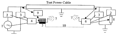
FIGURE 4 is a schematic diagram of an exemplary system for implementing the
disclosed methods/techniques;
FIGURES 5-7 are voltage plots for an exemplary homogenous cable according to
the
present disclosure;
=
=
=
7b
CA 02637487 2008-07-09
FIGURE 8 is a schematic diagram of an exemplary mixed cable configuration
according
to the present disclosure;
FIGURES 9-10 are voltage plots for an exemplary mixed cable configuration
according
to the present disclosure;
FIGURE 11 is a schematic diagram of an exemplary branched cable according to
the
present disclosure; and
FIGURES 12-14 are voltage amplitude plots for the exemplary branched cable at
three
distinct frequencies.
FIGURES 15-16 are exemplary "tomograms" of a cable having two defective areas
with
elevated tans and dielectric constant.
DESCRIPTION OF EXEMPLARY EMBODIMENT(S)
The disclosed cable diagnostic test methods, systems and apparatus utilize
"standing
wave" principles to identify and locate defect(s) along a power cable. As
described herein, the
disclosed methods/systems are effective in measuring dissipation factor (tans)
and dielectric
constant (6') associated with the insulation of a power cable, as well as the
resistance (Re) and
inductance (La) associated with the conductor system, at discrete points along
the cable's axial
length. The disclosed methods/systems offer significant advantages for cable
testing and related
defect identification/location.
With reference to FIG. 2(a), the schematic circuit diagram represents a
shielded power
cable insulation subjected to an alternating voltage source, V=Vmsin(cot),
where V., is the
amplitude of the voltage and o)=27cf is the angular frequency, f being the
frequency in Hz. The
cable insulation is shown as a pure capacitance, C, across which is connected
a resistance, R,
8
CA 02637487 2008-07-09
representing the dielectric losses. C is expressed in Farads and R in Ohms.
FIG. 2(b) is a
"phasor" diagram showing the current, Ic, drawn by the ideal capacitor, the
current, IR, drawn by
the resistor, and the total current I, which is the sum of the two previously
mentioned currents.
The angle, 8, between I and Ic is called the dissipation factor angle and
represents the effect of
the dielectric loss occurring in the cable insulation. The dissipation factor,
defined as tan6, can
be shown to be equal to 1/coRC.
An alternative equivalent notation, often used by physicists (as opposed to
engineers), is
as follows. The cable is assumed to be represented by the following complex
capacitance rather
than by a combination of a resistance in parallel with a capacitance: C* = Co
( s' - j E" ), where E'
is called the dielectric constant, E" the dissipation index, and Co the
geometric capacitance
(capacitance of the same cable construction having air as its insulating
medium) of the cable
insulation. The quantity "j" is the square root of the negative quantity "-F.
The current, I,
drawn by this complex capacitance is, therefore: I = V x jcoC = VcoCo (E" + j
s'). The phasor
diagram is redrawn in FIG.2(c) on the basis of this new form of the current,
I. The trigonometric
tangent of the angle 6, tano, is now expressed as the ratio E"/ E'. The
advantage of this notation
is that the axial tomography test would allow E' and E", as well as tan6, to
be determined. The
two previous representations are equivalent to each other in accordance with
the following
relationships:
C = E'Co and 1/R = coCoE"
The cable conductor is represented as a series combination of a frequency
dependent
resistance, Rc, and an inductive reactance, coLc as shown in FIG. 3(b).
9
CA 02637487 2008-07-09
Turning to FIG. 3(a), the voltage source at the sending end of the cable
supplies a
complex power, Sin, which is the sum of the real Power, Pin, and the reactive
power, Qin, related
to each other by the following relationship:
Sin = inx Iin* ¨ Pin + jQin [1]
The quantity Iin* denotes the complex conjugate of the input current, Tin. A
similar relationship
exists at the receiving, or load, end of the cable:
= VL x IL = PL jQL [2]
The complex power dissipated in the cable consists of two components, the
first is the
complex power, Sõ dissipated in the cable conductor, and the second is the
complex power, Sd,
dissipated in the dielectric material, or the insulation, of the cable. As a
cable ages, except in few
exceptional cases, the complex power dissipated in the conductor remains
constant, while that
dissipated in the cable insulation tends to increase. All existing global
diagnostic tests are
intended to determine the changes in the power dissipation of the cable
insulation. In the present
disclosure, the conductor impedance, Itc + joLõ is allowed to vary, as well,
along the cable axis.
Applying the principle of conservation of energy to this situation, the
complex power, Scl,
dissipated in the insulation, is found by the relationship:
Sd = Sin - SL Sc [3]
Splitting equation [3] into its real and imaginary components, the following
relationships
are obtained:
Pd= V12oCitan8i = V,20C0Ci = Pin - PL - Ii2Rci [4]
Qd = Vi2oCi = Vi20)C.E'i = Qin - QL - 1i2OLci
[5]
CA 02637487 2008-07-09
Equations similar to [4] and [5] can be written for various values of load
impedance, ZL,
source impedance, Zs and frequency, co. If the cable is divided into n
sections (not necessarily of
equal dimension), a minimum of n equations are needed to solve these
equations. The solution
will determine the values of tanS and C, or c' and s" for each section along
the cable axial length,
thus providing an axial tomogram of the cable insulation. The foregoing
process is typically
implemented in two distinct steps: first, the conductor is assumed to be
homogeneous and the
variations of insulation parameters are computed. On the basis of these
values, the voltage and
current profiles along the cable are re-calculated. In a second step,
equations [4] and [5] are
solved, assuming the calculated values of the insulation parameters are known,
while the
conductor parameters, Rc and Lõ are the unknown variables. Through an
iterative process, all
conductor and insulation parameters are calculated, such that four (4)
different axial tomograms
can be generated.
With this mathematical context, the systems and methods of the present
disclosure
establish the voltage and current profiles along the cable using the principle
of "standing waves."
For purposes of the disclosed methods/systems, standing wave principles are
utilized by
establishing an alternating voltage at relatively high frequency, generally on
the order of 10-1000
kilohertz (kHz) on the power cable to be tested. The voltage is connected
across the cable at the
"sending" end (see schematic depiction in FIG. 3(a)). This voltage sets up a
traveling wave
pattern, which is reflected at the opposite "receiving" end of the cable. The
combination of the
forward traveling wave and its reflection sets up a "standing wave" pattern
within the cable. Of
note, each cable section is subjected to an alternating voltage of frequency
co, but with different
amplitude. More particularly, a voltage wave travels from the voltage source
toward the load at
a velocity which is influenced by such parameters as the cable materials and
cable construction.
11
CA 02637487 2008-07-09
The forward moving voltage may be denoted as V. At the load, a portion of the
wave is
reflected, establishing a voltage V. The reflected portion of the voltage wave
is determined by
the value of the load impedance and the cable characteristic impedance. The
reflected portion of
the traveling wave can be determined mathematically if the load impedance, ZL,
connected at the
receiving end of the cable and the characteristic impedance, Zo, of the cable
are known. Once
the reflected portion of the traveling wave has been determined/calculated, it
is possible to
calculate the "standing wave" voltage and current at any point or section
along the axial length of
the cable. Indeed, at any point/section along the cable, the instantaneous
voltage (or current) is
the sum r + V- (or 1+ F) based on the waves traveling in the forward and
reflected directions,
respectively. Inasmuch as both waves are sinusoidal, the summation of the two
waves is also
sinusoidal.
The voltage and current patterns can be determined either through the
application of
conventional standing wave equations, or from the solution of the discrete
circuit representation
of FIG. 3(a), where the sections need not have the same length. Initially, the
values of voltage
and current are based on the global values of the cable parameters Rc, Lc, C
and R, obtained for
known load conditions, including short and open-circuit conditions, by direct
measurements of
voltage and current quantities at the sending and receiving cable ends. These
initial values of the
cable parameters can be modified, iteratively, as the solutions of equations
such as [4] and [5] are
obtained.
Absent changing conditions, the combination forms a wave that appears to be
stationary
(not moving or "standing" still). In reality, each point along the cable is
subjected to a sinusoidal
voltage of the same frequency as the source frequency; however, at each
point/section, the
amplitude of the resulting voltage is different. Each standing voltage wave is
also accompanied
12
CA 02637487 2008-07-09
by a standing current wave. With reference to FIGS. 5-7, experimental results
are plotted for an
exemplary homogeneous cable having the following characteristics/parameters
and test
conditions:
Length (L) = 200m
Wave velocity (u) = 160 m/i.ts
Frequency (f) = 200 kHz (FIG. 5); 400 kHz (FIGS. 6-7)
Wavelength (X) = 800m; 400m
Cable characteristic impedance (Z0) = 20S/
As shown in the foregoing plots, the voltage amplitude at various axial
positions along the cable
are calculated based on the test conditions according to the present
disclosure.
With reference to FIG. 8, an exemplary mixed cable configuration is
schematically
depicted. The mixed cable includes a first portion/component that is
fabricated from crosslinked
polyethylene (XLPE) and a second portion/component that is fabricated with an
oil-impregnated
paper-insulated lead-covered (PILC) cable. With reference to FIGS. 9-10,
experimental results
are plotted for the noted mixed cable configuration having the following
characteristics/parameters and test conditions:
PILC
Cable characteristic impedance (Zo) = 155-2
Length (L) = 600m
Wave velocity (u) = 140 m/us
XLPE
Cable characteristic impedance (Zo) = 18O
Length (L) = 200m
13
CA 02637487 2008-07-09
Wave velocity (u) = 160 m4is
Source Impedance
Rs = 0 or 15 SI
As shown in FIGS. 9-10, voltage amplitudes are measured/derived for various
points/sections along the length of the exemplary mixed cable configuration
described herein at
frequencies of 200kHz and 90kHz according to the present disclosure.
Turning to FIG. 11, a schematic diagram of an exemplary branched cable is
provided.
Incorporated into the schematic depiction of FIG. 11 are
characteristics/parameters associated
with an exemplary embodiment thereof. Voltage amplitudes for the exemplary
branched cable
are provided in the plots of FIGS. 12-14. As shown therein, voltage amplitudes
are
measured/derived for axial locations along the respective cable branches at
frequencies of
80kHz, 120kHz, and 160kHz.
By varying the load impedance, the source impedance or the frequency of the
voltage
source, or all three, a number of times (e.g., "n" times or more), the needed
equations to solve for
tan8; can be advantageously established. Of note, the dissipation factor at
these high frequencies
should not change significantly with a modest variation in frequency, and
therefore may be
assumed to be constant. However, this assumption is not a necessary condition
to apply the
disclosed method and, in further exemplary embodiments of the present
disclosure, potential
dissipation factor variations due to frequency variations may be included in
the mathematical
equations associated with the disclosed systems/methods. If necessary or
desired, the same
operation can be conducted by exchanging the sending end and the receiving end
of the cable,
generating half of the equations needed in each of these operations.
14
CA 02637487 2008-07-09
FIG. 15 and FIG. 16 are exemplary axial tomograms obtained on a 240m long
cable
model in which two areas with elevated tano = E"/E' and one area with elevated
dielectric
constant, E', were simulated.
The foregoing method allows the determination of a dissipation factor profile
along the
cable length using a broad range of excitation frequencies, e.g., frequencies
of 10-1000kHz. In
order to perform the disclosed axial tomography technique using significantly
lower frequencies,
e.g., frequencies of 50/60Hz, 1Hz or 0.1 Hz, or other, the amplitude Vm of the
excitation voltage
is generally modulated with the lower desired frequency. The result is an
"amplitude-
modulated" excitation source described mathematically as:
V = Vmsin(w Osin(wt) [6]
where 0i1 is the lower modulating frequency (e.g., 60Hz or 0.1Hz). With
appropriate circuitry
and/or software, the power associated with each of the two frequencies, w and
col, can be
separated. Thus, the dissipation factor profile at each of these frequencies
can be calculated
according to the mathematical techniques described above. The use of this
amplitude-modulated
technique allows "dielectric spectroscopy" to be performed by means of axial
tomography
(spectro-tomography).
Thus, in an exemplary embodiment, the disclosed cable detection
method/technique
involves the following steps:
(a) connecting an alternating voltage source to a cable at a "sending end"
thereof;
(b) applying a voltage to the cable at a first frequency to set up a
traveling wave along
the cable that is reflected at the "receiving end" thereof;
(c) permitting a standing wave pattern to be established along the cable by
the
traveling wave and the reflection thereof;
CA 02637487 2008-07-09
(d) measuring the total complex power loss (S,n) at the sending end of the
cable;
(e) measuring or calculating the complex power, (SO, dissipated in the load
impedance (4);
(f) repeating the foregoing steps while one of: (1) varying at least one of
(i) the load
impedance (ZL) connected at the receiving end of the cable, (ii) the first
frequency
of the voltage source, (iii) the output impedance of the voltage source, (iv)
a
combination of the load impedance (ZL), the output impedance of the voltage
source, and the first frequency of the voltage source, and (v) combinations
thereof, (2) interchanging sending and receiving cable ends and (3) a
combination
thereof;
(g) calculating the standing wave voltage at any point/section of the cable
based on
the load impedance (4) connected at the receiving end of the cable, and the
characteristic impedance (Zo) of the cable, or by solving the discrete circuit
model
of the cable as shown in FIG. 13(a), the global cable parameters, Rc, Lc, C
and R,
having been determined through measurements of voltage and current at the
sending and receiving cable ends under specific load conditions;
(h) calculating the complex power loss, Sc, in the conductor system;
(i) determining the dissipation factor, tano, and the dielectric constant,
c', at
predetermined points/sections along the axis of the cable;
re-calculating the voltage and current profiles according to the new values of
cable parameters;
16
CA 02637487 2008-07-09
(k) determining the values of conductor resistance (Rc) and
inductance (Lc)
(1) if warranted, repeating (g) through (k) with corrected cable
parameters.
The characteristic impedance, Zo, of the cable can be obtained through
theoretical
calculations or by direct measurement, according to one of the following
exemplary methods:
(1) Measuring the voltage, Vin, across the cable and the current, 'in, into
the cable at
the voltage source end while the load impedance is zero (short circuit) or
infinite
(open circuit). The short circuit impedance is defined as Zs, = Vin/Ii,, when
the
load is zero. The open circuit impedance is defined as Zoc = Vin/Iin when the
load
is infinite. The cable characteristic impedance is then equal to the square
root of
the product of Zse and Zoc.
(2) Changing the load impedance ZL until the voltage Vin at the source end
of the
cable and the voltage VL across the load are equal. This occurs when ZL is
equal
to Zo. The ratio of Z. and Zon can also be used to determine the propagation
constant of the cable (phase constant and attenuation) as well as velocity of
propagation, provided the cable length is known.
In a further exemplary embodiment of the present disclosure, the results
obtained by
partial discharge and axial tomography may be combined, thereby providing a
powerful
diagnostic tool that is vastly superior to all presently existing tools.
17
CA 02637487 2008-12-30
Mixed Cable Systems
The methods, systems and apparatus of the present disclosure also have
advantageous
applicability to mixed cable systems, i.e., cable systems where two or more
cable types, such as
extruded polymer and oil-impregnated laminated insulation, are interconnected
to each other.
These cables have different characteristic impedance, Zo, and velocity.
Equations can be written
based on each cable's "input impedance", Zin, its length, the velocity of the
electromagnetic
wave associated with it, and the frequency of the voltage source. These
equations will allow the
determination of the voltage at each point along the mixed cable system. The
velocity/cable
length can be measured from a time-domain reflectometry (TDR) test, as is
known from prior art
partial discharge tests performed by the applicant, or can be estimated by
calculation.
Branched Cable Systems
Cable systems with multiple branches can be successfully tested according to
the present
disclosure, provided a variable load impedance is connected to the end of each
branch. The
voltage calculations can, as well, be accomplished by means of the input
impedance formulas
described herein.
Hardware Configuration
An exemplary system configuration for practicing the methods/techniques of the
present
disclosure is illustrated in FIG. 4. In the schematic illustration of FIG. 4,
the noted components
are as follows:
Element 1: Remotely controllable, amplitude modulated variable frequency
voltage source;
Element 2: Current measuring device;
Element 3: Voltage measuring device;
18
CA 02637487 2008-07-09
Element 4: Digitizer;
Element 5: Microcomputer with means to communicate with
digitizer/receiver/transmitter
(element 6) by wireless or through power or optical cable;
Element 6: Digitizer/receiver/transmitter communicating with microcomputer
(element 5)
and/or control console (element 9) by wireless or through power/optical cable;
Element 7: Wireless communication system;
Element 8: Remotely controllable variable impedance;
Element 9: Operator remote control console;
Element 10: Fiber-optic communication system.
Thus, as schematically depicted in FIG. 4, at the near-end (or sending-end) of
the cable, the
system may include:
= A controllable variable frequency or amplitude-modulated variable
frequency (for the
spectro-tomography test) source with a variable series impedance, Zs;
= One or more devices for measuring the instantaneous voltage and current;
= A digitizer to digitize the measurements;
= A microcomputer to compute power and the voltage profile along the cable;
and
= A control console for the operator with means to communicate remotely
with the load-
end by wireless or through the power cable under test;
= Analog or digital filters, as needed, to separate the modulating
frequencies from the high
"carrier" frequencies.
At the remote-end, the following hardware is provided according to the
exemplary embodiment
depicted in FIG. 4:
= A remotely controllable load impedance,
19
CA 02637487 2015-07-08
= A voltage/current measuring device; and
= A digitizer and means to communicate with the near-end microcomputer by a
wireless system or through the power cable itself.
A computer/processor is generally provided to solve the set of "n" (or more)
equations
with "n" unknown quantities to yield the dissipation factor values at each of
the "n" sections of
the cable. The computer/processor is generally adapted to run system software
that is adapted to
calculate the voltage profile along the cable, the net power dissipated by the
cable insulation for
each setting of the load impedance, and the solution of the system of "n" (or
more) equations
with "n" unknown tano and e' values. In addition, the software will include
means to display the
tomograms (tans versus cable position) and to perform filtering operations on
the data. The
programming of such software is well within the skill of persons of ordinary
skill in the art,
based on the disclosure set forth herein as to the "n" (or more) equations to
be simultaneously
solved according to the present disclosure.
Although the methods, system and apparatus for diagnostic testing of cables
has been
described herein with reference to exemplary embodiments thereof, the present
disclosure is not
limited to such exemplary embodiments. The scope of the claims should not be
limited by the
preferred embodiments set forth in the examples, but should be given the
broadest interpretation
consistent with the description as a whole. Such variations, modifications and
enhancements are
expressly encompassed within the scope of the present disclosure.