Note: Descriptions are shown in the official language in which they were submitted.
CA 02730947 2012-08-30
-
SYSTEM AND METHOD FOR MANUFACTURING ARTHROPLASTY JIGS
HAVING IMPROVED MATING ACCURACY
[001]
FIELD OF THE INVENTION
[002] The present invention relates to systems and methods for
manufacturing customized arthroplasty cutting jigs. More specifically, the
present invention relates to automated systems and methods manufacturing
such jigs.
BACKGROUND OF THE INVENTION
[003] Over time and through repeated use, bones and joints can become
damaged or worn. For example, repetitive strain on bones and joints (e.g.,
through athletic activity), traumatic events, and certain diseases (e.g.,
arthritis)
can cause cartilage in joint areas, which normally provides a cushioning
effect, to wear down. When the cartilage wears down, fluid can accumulate in
the joint areas, resulting in pain, stiffness, and decreased mobility.
[004] Arthroplasty procedures can be used to repair damaged joints. During
a typical arthroplasty procedure, an arthritic or otherwise dysfunctional
joint
can be remodeled or realigned, or an implant can be implanted into the
damaged region. Arthroplasty procedures may take place in any of a number
of different regions of the body, such as a knee, a hip, a shoulder, or an
elbow.
[005] One type of arthroplasty procedure is a total knee arthroplasty ("TKA"),
in which a damaged knee joint is replaced with prosthetic implants. The knee
CA 02730947 2011-01-14
WO 2010/011590
PCT/US2009/051109
2
joint may have been damaged by, for example, arthritis (e.g., severe
osteoarthritis or degenerative arthritis), trauma, or a rare destructive joint
disease. During a TKA procedure, a damaged portion in the distal region of
the femur may be removed and replaced with a metal shell, and a damaged
portion in the proximal region of the tibia may be removed and replaced with a
channeled piece of plastic having a metal stem. In some TKA procedures, a
plastic button may also be added under the surface of the patella, depending
on the condition of the patella.
[006] Implants that are implanted into a damaged region may provide
support and structure to the damaged region, and may help to restore the
damaged region, thereby enhancing its functionality. Prior to implantation of
an implant in a damaged region, the damaged region may be prepared to
receive the implant. For example, in a knee arthroplasty procedure, one or
more of the bones in the knee area, such as the femur and/or the tibia, may
be treated (e.g., cut, drilled, reamed, and/or resurfaced) to provide one or
more surfaces that can align with the implant and thereby accommodate the
implant.
[007] Accuracy in implant alignment is an important factor to the success of a
TKA procedure. A one- to two-millimeter translational misalignment, or a one-
to two-degree rotational misalignment, may result in imbalanced ligaments,
and may thereby significantly affect the outcome of the TKA procedure. For
example, implant misalignment may result in intolerable post-surgery pain,
and also may prevent the patient from having full leg extension and stable leg
flexion.
[008] To achieve accurate implant alignment, prior to treating (e.g., cutting,
drilling, reaming, and/or resurfacing) any regions of a bone, it is important
to
correctly determine the location at which the treatment will take place and
how
the treatment will be oriented. In some methods, an arthroplasty jig may be
used to accurately position and orient a finishing instrument, such as a
cutting, drilling, reaming, or resurfacing instrument on the regions of the
bone.
The arthroplasty jig may, for example, include one or more apertures and/or
slots that are configured to accept such an instrument.
CA 02730947 2011-01-14
WO 2010/011590
PCT/US2009/051109
3
[009] A system and method has been developed for producing customized
arthroplasty jigs configured to allow a surgeon to accurately and quickly
perform an arthroplasty procedure that restores the pre-deterioration
alignment of the joint, thereby improving the success rate of such procedures.
Specifically, the customized arthroplasty jigs are indexed such that they
matingly receive the regions of the bone to be subjected to a treatment (e.g.,
cutting, drilling, reaming, and/or resurfacing). The customized arthroplasty
jigs are also indexed to provide the proper location and orientation of the
treatment relative to the regions of the bone. The indexing aspect of the
customized arthroplasty jigs allows the treatment of the bone regions to be
done quickly and with a high degree of accuracy that will allow the implants
to
restore the patient's joint to a generally pre-deteriorated state. However,
the
system and method for generating the customized jigs often relies on a
human to "eyeball" bone models on a computer screen to determine
configurations needed for the generation of the customized jigs. This is
"eyeballing" or manual manipulation of the bone modes on the computer
screen is inefficient and unnecessarily raises the time, manpower and costs
associated with producing the customized arthroplasty jigs. Furthermore, a
less manual approach may improve the accuracy of the resulting jigs.
[010] There is a need in the art for a system and method for reducing the
labor associated with generating customized arthroplasty jigs. There is also a
need in the art for a system and method for increasing the accuracy of
customized arthroplasty jigs.
SUMMARY
[011] Disclosed herein is a method of manufacturing an arthroplasty jig. In
one embodiment, the method includes: generating two-dimensional images
of at least a portion of a bone forming a joint; generating a first three-
dimensional computer model of the at least a portion of the bone from the
two-dimensional images; generating a second three-dimensional computer
model of the at least a portion of the bone from the two-dimensional images;
causing the first and second three-dimensional computer models to have in
CA 02730947 2011-01-14
WO 2010/011590
PCT/US2009/051109
4
common a reference position, wherein the reference position includes at least
one of a location and an orientation relative to an origin; generating a first
type
of data with the first three-dimensional computer model; generating a second
type of data with the second three-dimensional computer model; employing
the reference position to integrate the first and second types of data into an
integrated jig data; using the integrated jig data at a manufacturing device
to
manufacture the arthroplasty jig.
[012] Disclosed herein is a method of manufacturing an arthroplasty jig. In
one embodiment, the method includes: generating two-dimensional images
of at least a portion of a bone forming a joint; extending an open-loop
contour
line along an arthroplasty target region in at least some of the two-
dimensional images; generating a three-dimensional computer model of the
arthroplasty target region from the open-loop contour lines; generating from
the three-dimensional computer model surface contour data pertaining to the
arthroplasty target area; and using the surface contour data at a
manufacturing machine to manufacture the arthroplasty jig.
[013] Disclosed herein is a method of manufacturing an arthroplasty jig. In
one embodiment, the method includes: determining from an image at least
one dimension associated with a portion of a bone; comparing the at least one
dimension to dimensions of at least two candidate jig blank sizes; selecting
the smallest of the jig blank sizes that is sufficiently large to accommodate
the
at least one dimension; providing a jig blank of the selected size to a
manufacturing machine; and manufacturing the arthroplasty jig from the jig
blank.
[014] Disclosed herein are arthroplasty jigs manufactured according to any of
the aforementioned methods of manufacture. In some embodiments, the
arthroplasty jigs may be indexed to matingly receive arthroplasty target
regions of a joint bone. The arthroplasty jigs may also be indexed to orient
saw cut slots and drill hole guides such that when the arthroplasty target
regions are matingly received by the arthroplasty jig, the saw cuts and drill
holes administered to the arthroplasty target region via the saw cut slots and
CA 02730947 2011-01-14
WO 2010/011590
PCT/US2009/051109
drill hole guides will facilitate arthroplasty implants generally restoring
the joint
to a pre-degenerated state (i.e., natural alignment state).
[015] Disclosed herein is a method of computer generating a three-
dimensional surface model of an arthroplasty target region of a bone forming
a joint. In one embodiment, the method includes: generating two-
dimensional images of at least a portion of the bone; generating an open-loop
contour line along the arthroplasty target region in at least some of the two-
dimensional images; and generating the three-dimensional model of the
arthroplasty target region from the open-loop contour lines.
[016] Disclosed herein is a method of generating a three-dimensional
arthroplasty jig computer model. In one embodiment, the method includes:
comparing a dimension of at least a portion of a bone of a joint to candidate
jig blank sizes; and selecting from the candidate jig blank sizes a smallest
jig
blank size able to accommodate the dimensions of the at least a portion of the
bone.
[017] Disclosed herein is a method of generating a three-dimensional
arthroplasty jig computer model. In one embodiment, the method includes:
forming an interior three-dimensional surface model representing an
arthroplasty target region of at least a portion of a bone; forming an
exterior
three-dimensional surface model representing an exterior surface of a jig
blank; and combining the interior surface model and exterior surface model to
respectively form the interior surface and exterior surface of the three-
dimensional arthroplasty jig computer model.
[018] Disclosed herein is a method of generating a production file associated
with the manufacture of arthroplasty jigs. The method includes: generating
first data associated a surface contour of an arthroplasty target region of a
joint bone; generating second data associated with at least one of a saw cut
and a drill hole to be administered to the arthroplasty target region during
an
arthroplasty procedure; and integrating first and second data, wherein a
positional relationship of first data relative to an origin and a positional
relationship of second data relative to the origin are coordinated with each
CA 02730947 2011-01-14
WO 2010/011590
PCT/US2009/051109
6
other to be generally identical during the respective generations of first and
second data.
[019] Disclosed herein is a method of defining a mating surface in a first
side
of an arthroplasty jig. The mating surface is configured to matingly receive
and contact a corresponding patient surface including at least one of a bone
surface and a cartilage surface. The first side is oriented towards the
patient
surface when the mating surface matingly receives and contacts the patient
surface. In one embodiment, the method includes: a) identifying a contour
line associated with the patient surface as represented in a medical image; b)
evaluating via an algorithm the adequacy of the contour line for defining a
portion of the mating surface associated with the contour line; c) modifying
the contour line if the contour line is deemed inadequate; and d) employing
the modified contour line to define the portion of the mating surface
associated with the contour line.
[020] Disclosed herein is an arthroplasty jig for assisting in the performance
of an arthroplasty procedure associated with a patient surface including at
least one of a bone surface and a cartilage surface. In one embodiment, the
jig may include a first side, a second side generally opposite the first side,
and
a mating surface in the first side and configured to matingly receive and
contact at least a portion of the patient surface. The first side may be
configured to be oriented towards the patient surface when the mating surface
matingly receives and contacts the patient surface. The mating surface may
be defined according to the following process steps: a) identifying a contour
line associated with the patient surface as represented in a medical image; b)
evaluating via an algorithm the adequacy of the contour line for defining a
portion of the mating surface associated with the contour line; c) modifying
the contour line if the contour line is deemed inadequate; and d) employing
the modified contour line to define the portion of the mating surface
associated with the contour line.
[021] Disclosed herein is a femoral arthroplasty jig for assisting in the
performance of a femoral arthroplasty procedure on a femoral arthroplasty
target region. In one embodiment the jig includes a first side, a second side
CA 02730947 2011-01-14
WO 2010/011590
PCT/US2009/051109
7
generally opposite the first side; and a mating surface in the first side and
configured to matingly receive and contact certain surfaces of the femoral
arthroplasty target region. The certain surfaces may bed limited to a medial
articular condyle surface, a lateral articular condyle surface, and a
generally
planar area of an anterior side of a femoral shaft. The first side may be
configured to be oriented towards the femoral arthroplasty target region
surface when the mating surface matingly receives and contacts the certain
surfaces.
[022] Disclosed herein is a tibial arthroplasty jig for assisting in the
performance of a tibial arthroplasty procedure on a tibial arthroplasty target
region. In one embodiment, the jig includes a first side, a second side
generally opposite the first side, and a mating surface. The mating surface
may be in the first side and configured to matingly receive and contact
certain
surfaces of the tibial arthroplasty target region. The certain surfaces may be
limited to a medial articular plateau surface, a lateral articular plateau
surface,
and a generally planar area of an anterior side of a tibial shaft. The first
side
may be configured to be oriented towards the tibial arthroplasty target region
surface when the mating surface matingly receives and contacts the certain
surfaces.
[023] Disclosed herein is a tibial arthroplasty jig for assisting in the
performance of a tibial arthroplasty procedure on a tibial arthroplasty target
region. In one embodiment, the jig includes a first side, a second side
generally opposite the first side. The second side may include a mating
surface in the first side. The mating surface may be configured to matingly
receive and contact a generally planar area of an anterior side of a tibial
shaft
distal of the tibial plateau edge and generally proximal of the tibial
tuberosity.
The first side may be configured to be oriented towards the tibial
arthroplasty
target region surface when the mating surface matingly receives and contacts
the planar area.
[024] Disclosed herein is a femoral arthroplasty jig for assisting in the
performance of a femoral arthroplasty procedure on a femoral arthroplasty
target region. In one embodiment, the jig includes a first side, a second side
CA 02730947 2011-01-14
WO 2010/011590
PCT/US2009/051109
8
generally opposite the first side, and a mating surface in the first side. The
mating surface may be configured to matingly receive and contact a generally
planar area of an anterior side of a femoral shaft generally proximal of the
patellar facet boarder and generally distal an articularis genu. The first
side
may be configured to be oriented towards the femoral arthroplasty target
region surface when the mating surface matingly receives and contacts the
planar area.
[025] While multiple embodiments are disclosed, still other embodiments of
the present invention will become apparent to those skilled in the art from
the
following detailed description, which shows and describes illustrative
embodiments of the invention. As will be realized, the invention is capable of
modifications in various aspects, all without departing from the spirit and
scope of the present invention. Accordingly, the drawings and detailed
description are to be regarded as illustrative in nature and not restrictive.
BRIEF DESCRIPTION OF THE DRAWINGS
[026] FIG. 1A is a schematic diagram of a system for employing the
automated jig production method disclosed herein.
[027] FIGS. 1B-1E are flow chart diagrams outlining the jig production
method disclosed herein.
[028] FIGS. 1F and 1G are, respectively, bottom and top perspective views
of an example customized arthroplasty femur jig.
[029] FIGS. 1H and 1 I are, respectively, bottom and top perspective views
of an example customized arthroplasty tibia jig.
[030] FIG. 2A is an anterior-posterior image slice of the damaged lower or
knee joint end of the patient's femur, wherein the image slice includes an
open-loop contour line segment corresponding to the targeted region of the
damaged lower end.
[031] FIG. 2B is a plurality of image slices with their respective open-loop
contour line segments, the open-loop contour line segments being
accumulated to generate the 3D model of the targeted region.
CA 02730947 2011-01-14
WO 2010/011590
PCT/US2009/051109
9
[032] FIG. 2C is a 3D model of the targeted region of the damaged lower end
as generated using the open-loop contour line segments depicted in FIG. 2B.
[033] FIG. 2D is an anterior-posterior image slice of the damaged lower or
knee joint end of the patient's femur, wherein the image slice includes a
closed-loop contour line corresponding to the femur lower end, including the
targeted region.
[034] FIG. 2E is a plurality of image slices with their respective closed-loop
contour line segments, the closed-loop contour lines being accumulated to
generate the 3D model of the femur lower end, including the targeted region.
[035] FIG. 2F is a 3D model of the femur lower end, including the targeted
region, as generated using the closed-loop contour lines depicted in FIG. 2B.
[036] FIG. 2G is a flow chart illustrating an overview of the method of
producing a femur jig.
[037] FIG. 3A is a top perspective view of a left femoral cutting jig blank
having predetermined dimensions.
[038] FIG. 3B is a bottom perspective view of the jig blank depicted in FIG.
3A.
[039] FIG. 3C is plan view of an exterior side or portion of the jig blank
depicted in FIG. 3A.
[040] FIG. 4A is a plurality of available sizes of left femur jig blanks, each
depicted in the same view as shown in FIG. 3C.
[041] FIG. 4B is a plurality of available sizes of right femur jig blanks,
each
depicted in the same view as shown in FIG. 3C.
[042] FIG. 5 is an axial view of the 3D surface model or arthritic model of
the
patient's left femur as viewed in a direction extending distal to proximal.
[043] FIG. 6 depicts the selected model jig blank of FIG. 3C superimposed
on the model femur lower end of FIG. 5.
CA 02730947 2011-01-14
WO 2010/011590
PCT/US2009/051109
[044] FIG. 7A is an example scatter plot for selecting from a plurality of
candidate jig blanks sizes a jig blank size appropriate for the lower end of
the
patient's femur.
[045] FIG. 7B is a flow diagram illustrating an embodiment of a process of
selecting an appropriately sized jig blank.
[046] FIG. 8A is an exterior perspective view of a femur jig blank exterior
surface model.
[047] FIG. 8B is an interior perspective view of the femur jig blank exterior
surface model of FIG. 8A.
[048] FIG. 9A is a perspective view of the extracted jig blank exterior
surface
model being combined with the extracted femur surface model.
[049] FIG. 9B is a perspective view of the extracted jig blank exterior
surface
model combined with the extracted femur surface model.
[050] FIG. 9C is a cross section of the combined jig blank exterior surface
model and the femur surface model as taken along section line 9C-9C in FIG.
9B.
[051] FIG. 10A is an exterior perspective view of the resulting femur jig
model.
[052] FIG. 10B is an interior perspective view of the femur jig model of FIG.
10A.
[053] FIG. 11 illustrates a perspective view of the integrated jig model
mating
with the "arthritic model".
[054] FIG. 12A is an anterior-posterior image slice of the damaged upper or
knee joint end of the patient's tibia, wherein the image slice includes an
open-
loop contour line segment corresponding to the target area of the damaged
upper end.
[055] FIG. 12B is a plurality of image slices with their respective open-loop
contour line segments, the open-loop contour line segments being
accumulated to generate the 3D model of the target area.
CA 02730947 2011-01-14
WO 2010/011590
PCT/US2009/051109
11
[056] FIG. 12C is a 3D model of the target area of the damaged upper end
as generated using the open-loop contour line segments depicted in FIG.
12B.
[057] FIG. 13A is a top perspective view of a right tibia cutting jig blank
having predetermined dimensions.
[058] FIG. 13B is a bottom perspective view of the jig blank depicted in FIG.
13A.
[059] FIG. 13C is plan view of an exterior side or portion of the jig blank
depicted in FIG. 13A.
[060] FIG. 14A is a plurality of available sizes of right tibia jig blanks,
each
depicted in the same view as shown in FIG. 13C.
[061] FIG. 14B is a plurality of available sizes of left tibia jig blanks,
each
depicted in the same view as shown in FIG. 13C.
[062] FIG. 15 is an axial view of the 3D surface model or arthritic model of
the patient's right tibia as viewed in a direction extending proximal to
distal.
[063] FIG. 16 depicts the selected model jig blank of FIG. 13C superimposed
on the model tibia upper end of FIG. 15.
[064] FIG. 17A is an example scatter plot for selecting from a plurality of
candidate jig blanks sizes a jig blank size appropriate for the upper end of
the
patient's tibia.
[065] FIG. 17B is a flow diagram illustrating an embodiment of a process of
selecting an appropriately sized jig blank.
[066] FIG. 18A is an exterior perspective view of a tibia jig blank exterior
surface model.
[067] FIG. 18B is an interior perspective view of the tibia jig blank exterior
surface model of FIG. 18A.
[068] FIG. 19A is a perspective view of the extracted jig blank exterior
surface model being combined with the extracted tibia surface model.
CA 02730947 2011-01-14
WO 2010/011590
PCT/US2009/051109
12
[069] FIGS. 19B-19D are perspective views of the extracted jig blank exterior
surface model combined with the extracted tibia surface model.
[070] FIG. 20A is an exterior perspective view of the resulting tibia jig
model.
[071] FIG. 20B is an interior perspective view of the tibia jig model of FIG.
20A.
[072] FIG. 21 illustrates a perspective view of the integrated jig model
mating
with the "arthritic model".
[073] FIG. 22A illustrates the distal axial view of the 3D model of the
patient's
femur shown in FIG. 5 with the contour lines of the image slices shown and
spaced apart by the thickness DT of the slices.
[074] FIG. 22B represents a coronal view of a 3D model of the patient's
femur with the contour lines of the image slices shown and spaced apart by
the thickness DT of the slices.
[075] FIG. 23 illustrates an example sagittal view of compiled contour lines
of
successive sagittal 2D MRI images based on the slices shown in FIGS. 22A-B
with a slice thickness DT of 2 mm.
[076] FIG. 24 illustrates an example contour line of one of the contour lines
depicted in FIGS. 22A-23, wherein the contour line is depicted in a sagittal
view and is associated with an image slice of the femoral condyle.
[077] FIG. 25 represents an example overestimation algorithm that may be
used to identify and adjust for irregular contour line regions when forming
the
3D model.
[078] FIG. 26 depicts implementing an example analysis scheme (according
to block 2506) on the irregular contour line region 2402B of FIG. 24.
[079] FIG. 27 depicts the irregular region 2402B from FIG. 26 including a
proposed area of overestimation, wherein an overestimation procedure
creates an adjusted contour line and positionally deviates the adjusted
contour line from the original surface profile contour line.
CA 02730947 2011-01-14
WO 2010/011590
PCT/US2009/051109
13
[080] FIG. 28 illustrates the example analysis scheme according to the
algorithm of FIG. 25 implemented on the irregular region 2402C from FIG. 24
where an irregular surface of the condylar contour is observed.
[081] FIG. 29A depicts the irregular region 2402C from FIG. 28 including a
proposed area of overestimation indicated by the dashed line areas 2902A-B.
[082] FIG. 29B is similar to FIG. 29A, except depicting a tool with a larger
diameter.
[083] FIG. 29C is similar to FIG. 29B, except depicting a tool with a larger
diameter.
[084] FIG. 30 depicts the irregular region 2402D from FIG. 24 including a
proposed area of overestimation indicated by the dashed line.
[085] FIG. 31 shows an analysis of the regular region 2402A from FIG. 24.
[086] FIG. 32A is a diagrammatic sagittal-coronal-distal isometric view of
three contour lines of three adjacent image slices depicting angular
relationships that may be used to determine whether portions of the one or
more contour lines may be employed to generate 3D computer models.
[087] FIGS. 32B-G are example right triangles that may be used for
determining the angular deviation 0 between corresponding coordinate points
of contour lines of adjacent image slices per block 2514 of FIG. 25.
[088] FIG. 33A depicts portions of contour lines nth, nth+1, nth+2, nth+3 and
nth+4
in a sagittal view similar to that of FIG. 23.
[089] FIG. 33B is a bone surface contour line and a linear interpolation bone
surface contour line as viewed along a section line 33B-33B transverse to
image slices containing the contour lines nth, nth+1, nth+2,
nth+-3
and nth+4 of FIG.
33A.
[090] FIG. 33C depicts portions of contour lines nth, nth+1, nth+2, n_th+3 and
nth+4
in a sagittal view similar to that of FIG. 23.
[091] FIG. 33D is a bone surface contour line and a linear interpolation bone
surface contour line as viewed along a section line 33D-33D transverse to
CA 02730947 2011-01-14
WO 2010/011590
PCT/US2009/051109
14
image slices containing the contour lines nth, nth+1, nth+2, nth+3 and nth+4
of FIG.
33C.
[092] FIG. 33E depicts portions of contour lines nth, nth+1, nth+2, nth+3 and
nth+4
in a sagittal view similar to that of FIG. 23.
[093] FIG. 33F is a bone surface contour line and a linear interpolation bone
surface contour line as viewed along a section line 33F-33F transverse to
image slices containing the contour lines nth, nth, nth+2, nth+3 and th+4 of
FIG.
33E.
[094] FIG. 34 is a distal view similar to that of FIG. 5 depicting contour
lines
produced by imaging the right femur at an image spacing DT of, for example,
2 mm.
[095] FIGS. 35-38 are sagittal views of the contour lines of respective
regions of FIG. 34.
[096] FIG. 39A is distal-sagittal isometric view of a femoral distal end.
[097] FIG. 39B is a bottom perspective view of an example customized
arthroplasty femur jig that has been generated via the overestimation process
disclosed herein.
[098] FIG. 39C is an anterior-posterior cross-section of the femur jig of FIG.
39B mounted on the femur distal end of FIG. 39A.
[099] FIG. 39D is a coronal view of the anterior side of the femoral distal
end.
[0100] FIG. 40 depicts closed-loop contour lines that are image segmented
from image slices, wherein the contour lines outline the cortical bone surface
of the lower end of the femur.
[0101]FIG. 41A illustrates the proximal axial view of the 3D model of the
patient's tibia shown in FIG. 15 with the contour lines of the image slices
shown and spaced apart by the thickness DT of the slices.
[0102] FIG. 41B represents a coronal view of a 3D model of the patient's tibia
with the contour lines of the image slices shown and spaced apart by the
thickness DT of the slices.
CA 02730947 2011-01-14
WO 2010/011590
PCT/US2009/051109
[0103] FIG. 42 illustrates an example sagittal view of compiled contour lines
of
successive sagittal 2D MRI images based on the slices shown in FIGS. 41A-B
with a slice thickness DT of 2 mm.
[0104] FIG. 43 illustrates an example contour line of one of the contour lines
depicted in FIGS. 41A-42, wherein the contour line is depicted in a sagittal
view and is associated with an image slice of the tibia plateau.
[0105] FIG. 44 depicts implementing an example analysis scheme (according
to block 2506) on the irregular contour line region 4302B of FIG. 43.
[0106] FIG. 45 depicts the irregular region 4302B from FIG. 44 including a
proposed area of overestimation, wherein an overestimation procedure
creates an adjusted contour line and positionally deviates the adjusted
contour line from the original surface profile contour line.
[0107] FIGS. 46A and 46B show an analysis of the regular regions 4302A and
4302C from FIG. 43.
[0108] FIG. 47 is a distal view similar to that of FIG. 15 depicting contour
lines
produced by imaging the left tibia at an image spacing DT of, for example, 2
MM.
[0109] FIGS. 48-51 are sagittal views of the contour lines of respective
regions of FIG. 47.
[0110] FIG. 52A is distal-sagittal isometric view of a tibial proximal end.
[0111] FIGS. 52B-C are, respectively, top and bottom perspective views of an
example customized arthroplasty tibia jig that has been generated via the
overestimation process disclosed herein.
[0112] FIG. 52D is an anterior-posterior cross-section of the tibia jig of
FIGS.
52B-C mounted on the tibia proximal end of FIG. 52A.
[0113] FIG. 52E is a coronal view of the anterior side of the tibial proximal
end.
CA 02730947 2011-01-14
WO 2010/011590
PCT/US2009/051109
16
[0114] FIG. 53 depicts closed-loop contour lines that are image segmented
from image slices, wherein the contour lines outline the cortical bone surface
of the upper end of the tibia.
[0115] FIG. 54 is an anterior isometric view of the femur distal end.
[0116] FIG. 55 is an anterior isometric view of the tibia proximal end.
DETAILED DESCRIPTION
[0117] Disclosed herein are customized arthroplasty jigs 2 and systems 4 for,
and methods of, producing such jigs 2. The jigs 2 are customized to fit
specific bone surfaces of specific patients. Depending on the embodiment
and to a greater or lesser extent, the jigs 2 are automatically planned and
generated and may be similar to those disclosed in these three U.S. Patent
Applications: U.S. Patent Application 11/656,323 to Park et al., titled
"Arthroplasty Devices and Related Methods" and filed January 19, 2007; U.S.
Patent Application 10/146,862 to Park et al., titled "Improved Total Joint
Arthroplasty System" and filed May 15, 2002; and U.S. Patent 11/642,385 to
Park et al., titled "Arthroplasty Devices and Related Methods" and filed
December 19, 2006. The disclosures of these three U.S. Patent Applications
are incorporated by reference in their entireties into this Detailed
Description.
[0118] a. Overview of System and Method for Manufacturing Customized
Arthroplasty Cutting Jigs
[0119] For an overview discussion of the systems 4 for, and methods of,
producing the customized arthroplasty jigs 2, reference is made to FIGS. 1A-
1E. FIG. 1A is a schematic diagram of a system 4 for employing the
automated jig production method disclosed herein. FIGS. 1B-1E are flow
chart diagrams outlining the jig production method disclosed herein. The
following overview discussion can be broken down into three sections.
[0120] The first section, which is discussed with respect to FIG. 1A and
[blocks 100-125] of FIGS. 1B-1E, pertains to an example method of
determining, in a three-dimensional ("3D") computer model environment, saw
cut and drill hole locations 30, 32 relative to 3D computer models that are
CA 02730947 2011-01-14
WO 2010/011590
PCT/US2009/051109
17
termed restored bone models 28. The resulting "saw cut and drill hole data"
44 is referenced to the restored bone models 28 to provide saw cuts and drill
holes that will allow arthroplasty implants to restore the patient's joint to
its
pre-degenerated state or, in other words, its natural alignment state.
[0121]The second section, which is discussed with respect to FIG. 1A and
[blocks 100-105 and 130-145] of FIGS. 1B-1E, pertains to an example method
of importing into 3D computer generated jig models 38 3D computer
generated surface models 40 of arthroplasty target areas 42 of 3D computer
generated arthritic models 36 of the patient's joint bones. The resulting "jig
data" 46 is used to produce a jig customized to matingly receive the
arthroplasty target areas of the respective bones of the patient's joint.
[0122]The third section, which is discussed with respect to FIG. 1A and
[blocks 150-165] of FIG. 1E, pertains to a method of combining or integrating
the "saw cut and drill hole data" 44 with the "jig data" 46 to result in
"integrated
jig data" 48. The "integrated jig data" 48 is provided to the CNC machine 10
for the production of customized arthroplasty jigs 2 from jig blanks 50
provided
to the CNC machine 10. The resulting customized arthroplasty jigs 2 include
saw cut slots and drill holes positioned in the jigs 2 such that when the jigs
2
matingly receive the arthroplasty target areas of the patient's bones, the cut
slots and drill holes facilitate preparing the arthroplasty target areas in a
manner that allows the arthroplasty joint implants to generally restore the
patient's joint line to its pre-degenerated or natural alignment state.
[0123]As shown in FIG. 1A, the system 4 includes a computer 6 having a
CPU 7, a monitor or screen 9 and an operator interface controls 11. The
computer 6 is linked to a medical imaging system 8, such as a CT or MRI
machine 8, and a computer controlled machining system 10, such as a CNC
milling machine 10.
[0124]As indicated in FIG. 1A, a patient 12 has a joint 14 (e.g., a knee,
elbow,
ankle, wrist, hip, shoulder, skull/vertebrae or vertebrae/vertebrae interface,
etc.) to be replaced. The patient 12 has the joint 14 scanned in the imaging
machine 8. The imaging machine 8 makes a plurality of scans of the joint 14,
wherein each scan pertains to a thin slice of the joint 14.
CA 02730947 2011-01-14
WO 2010/011590
PCT/US2009/051109
18
[0125] As can be understood from FIG. 1B, the plurality of scans is used to
generate a plurality of two-dimensional ("2D") images 16 of the joint 14
[block
1001. Where, for example, the joint 14 is a knee 14, the 2D images will be of
the femur 18 and tibia 20. The imaging may be performed via CT or MRI. In
one embodiment employing MRI, the imaging process may be as disclosed in
U.S. Patent Application 11/946,002 to Park, which is entitled "Generating MRI
Images Usable For The Creation Of 3D Bone Models Employed To Make
Customized Arthroplasty Jigs," was filed November 27, 2007 and is
incorporated by reference in its entirety into this Detailed Description.
[0126] As can be understood from FIG. 1A, the 2D images are sent to the
computer 6 for creating computer generated 3D models. As indicated in FIG.
1B, in one embodiment, point Pis identified in the 2D images 16 [block 1051.
In one embodiment, as indicated in [block 105] of FIG. 1A, point P may be at
the approximate medial-lateral and anterior-posterior center of the patient's
joint 14. In other embodiments, point P may be at any other location in the 2D
images 16, including anywhere on, near or away from the bones 18, 20 or the
joint 14 formed by the bones 18, 20.
[0127]As described later in this overview, point P may be used to locate the
computer generated 3D models 22, 28, 36 created from the 2D images 16
and to integrate information generated via the 3D models. Depending on the
embodiment, point P, which serves as a position and/or orientation reference,
may be a single point, two points, three points, a point plus a plane, a
vector,
etc., so long as the reference P can be used to position and/or orient the 3D
models 22, 28, 36 generated via the 2D images 16.
[0128]As shown in FIG. 1C, the 2D images 16 are employed to create
computer generated 3D bone-only (i.e., "bone models") 22 of the bones 18,
20 forming the patient's joint 14 [block 110]. The bone models 22 are located
such that point P is at coordinates (Xo-J, Yo-i, Zo_i) relative to an origin
(Xo, Yo,
Zo) of an X-Y-Z axis [block 110]. The bone models 22 depict the bones 18, 20
in the present deteriorated condition with their respective degenerated joint
surfaces 24, 26, which may be a result of osteoarthritis, injury, a
combination
thereof, etc.
CA 02730947 2011-01-14
WO 2010/011590
PCT/US2009/051109
19
[01291 Computer programs for creating the 3D computer generated bone
models 22 from the 2D images 16 include: Analyze from AnalyzeDirect, Inc.,
Overland Park, KS; Insight Toolkit, an open-source software available from
the National Library of Medicine Insight Segmentation and Registration Toolkit
("ITK"), vvww.itk.org; 3D Slicer, an open¨source software available from
www.slicer.org; Mimics from Materialise, Ann Arbor, MI; and Paraview
available at www.paraview.org.
[0130]As indicated in FIG. 1C, the 3D computer generated bone models 22
are utilized to create 3D computer generated "restored bone models" or
"planning bone models" 28 wherein the degenerated surfaces 24, 26 are
modified or restored to approximately their respective conditions prior to
degeneration [block 115]. Thus, the bones 18,20 of the restored bone
models 28 are reflected in approximately their condition prior to
degeneration.
The restored bone models 28 are located such that point P is at coordinates
(Xol, YcH, Zo) relative to the origin (Xo, Yo, Zo). Thus, the restored bone
models 28 share the same orientation and positioning relative to the origin
(X0, Yo, Zo) as the bone models 22.
[0131]In one embodiment, the restored bone models 28 are manually created
from the bone models 22 by a person sitting in front of a computer 6 and
visually observing the bone models 22 and their degenerated surfaces 24, 26
as 3D computer models on a computer screen 9. The person visually
observes the degenerated surfaces 24, 26 to determine how and to what
extent the degenerated surfaces 24, 26 surfaces on the 3D computer bone
models 22 need to be modified to restore them to their pre-degenerated
condition. By interacting with the computer controls 11, the person then
manually manipulates the 3D degenerated surfaces 24, 26 via the 3D
modeling computer program to restore the surfaces 24, 26 to a state the
person believes to represent the pre-degenerated condition. The result of this
manual restoration process is the computer generated 3D restored bone
models 28, wherein the surfaces 24', 26' are indicated in a non-degenerated
state.
CA 02730947 2011-01-14
WO 2010/011590
PCT/US2009/051109
[0132]In one embodiment, the above-described bone restoration process is
generally or completely automated. In other words, a computer program may
analyze the bone models 22 and their degenerated surfaces 24, 26 to
determine how and to what extent the degenerated surfaces 24, 26 surfaces
on the 3D computer bone models 22 need to be modified to restore them to
their pre-degenerated condition. The computer program then manipulates the
3D degenerated surfaces 24, 26 to restore the surfaces 24, 26 to a state
intended to represent the pre-degenerated condition. The result of this
automated restoration process is the computer generated 3D restored bone
models 28, wherein the surfaces 24', 26' are indicated in a non-degenerated
state.
[0133]As depicted in FIG. 1C, the restored bone models 28 are employed in a
pre-operative planning ("POP") procedure to determine saw cut locations 30
and drill hole locations 32 in the patient's bones that will allow the
arthroplasty
joint implants to generally restore the patient's joint line to it pre-
degenerative
alignment [block 120].
[0134] In one embodiment, the POP procedure is a manual process, wherein
computer generated 3D implant models 34 (e.g., femur and tibia implants in
the context of the joint being a knee) and restored bone models 28 are
manually manipulated relative to each other by a person sitting in front of a
computer 6 and visually observing the implant models 34 and restored bone
models 28 on the computer screen 9 and manipulating the models 28, 34 via
the computer controls 11. By superimposing the implant models 34 over the
restored bone models 28, or vice versa, the joint surfaces of the implant
models 34 can be aligned or caused to correspond with the joint surfaces of
the restored bone models 28. By causing the joint surfaces of the models 28,
34 to so align, the implant models 34 are positioned relative to the restored
bone models 28 such that the saw cut locations 30 and drill hole locations 32
can be determined relative to the restored bone models 28.
[0135] In one embodiment, the POP process is generally or completely
automated. For example, a computer program may manipulate computer
generated 3D implant models 34 (e.g., femur and tibia implants in the context
CA 02730947 2011-01-14
WO 2010/011590
PCT/US2009/051109
21
of the joint being a knee) and restored bone models or planning bone models
28 relative to each other to determine the saw cut and drill hole locations
30,
32 relative to the restored bone models 28. The implant models 34 may be
superimposed over the restored bone models 28, or vice versa. In one
embodiment, the implant models 34 are located at point P' (X0-k, YO-k, ZO-k)
relative to the origin (X0, Yo, Zo), and the restored bone models 28 are
located
at point P (Xo, Yo-j, Zol). To cause the joint surfaces of the models 28, 34
to
correspond, the computer program may move the restored bone models 28
from point P (Xo, Yo-j, Z01) to point P' (X0-k, YO-k, ZO-k), or vice versa.
Once the
joint surfaces of the models 28, 34 are in close proximity, the joint surfaces
of
the implant models 34 may be shape-matched to align or correspond with the
joint surfaces of the restored bone models 28. By causing the joint surfaces
of the models 28, 34 to so align, the implant models 34 are positioned
relative
to the restored bone models 28 such that the saw cut locations 30 and drill
hole locations 32 can be determined relative to the restored bone models 28.
[0136]As indicated in FIG. 1E, in one embodiment, the data 44 regarding the
saw cut and drill hole locations 30, 32 relative to point P' (X0-k, YO-k, Zo-
k) is
packaged or consolidated as the "saw cut and drill hole data" 44 [block 145].
The "saw cut and drill hole data" 44 is then used as discussed below with
respect to [block 150] in FIG. 1E.
[0137]As can be understood from FIG. 1D, the 2D images 16 employed to
generate the bone models 22 discussed above with respect to [block 1101 of
FIG. 1C are also used to create computer generated 3D bone and cartilage
models (i.e., "arthritic models") 36 of the bones 18,20 forming the patient's
joint 14 [block 130]. Like the above-discussed bone models 22, the arthritic
models 36 are located such that point P is at coordinates (Xo, Yo.i, Zo.)
relative to the origin (Xo, Yo, Zo) of the X-Y-Z axis [block 130]. Thus, the
bone
and arthritic models 22, 36 share the same location and orientation relative
to
the origin (Xo, Yo, Zo). This position/orientation relationship is generally
maintained throughout the process discussed with respect to FIGS 1B-1E.
Accordingly, movements relative to the origin (Xo, Yo, Zo) of the bone models
22 and the various descendants thereof (i.e., the restored bone models 28,
CA 02730947 2011-01-14
WO 2010/011590
PCT/US2009/051109
22
bone cut locations 30 and drill hole locations 32) are also applied to the
arthritic models 36 and the various descendants thereof (i.e., the jig models
38). Maintaining the position/orientation relationship between the bone
models 22 and arthritic models 36 and their respective descendants allows
the "saw cut and drill hole data" 44 to be integrated into the "jig data" 46
to
form the "integrated jig data" 48 employed by the CNC machine 10 to
manufacture the customized arthroplasty jigs 2.
[0138]Computer programs for creating the 3D computer generated arthritic
models 36 from the 2D images 16 include: Analyze from AnalyzeDirect, Inc.,
Overland Park, KS; Insight Toolkit, an open-source software available from
the National Library of Medicine Insight Segmentation and Registration Toolkit
("ITK"), www.itk.org; 3D Slicer, an open¨source software available from
www.slicer.org; Mimics from Materialise, Ann Arbor, MI; and Paraview
available at www.paraview.org.
[0139]Similar to the bone models 22, the arthritic models 36 depict the bones
18, 20 in the present deteriorated condition with their respective degenerated
joint surfaces 24, 26, which may be a result of osteoarthritis, injury, a
combination thereof, etc. However, unlike the bone models 22, the arthritic
models 36 are not bone-only models, but include cartilage in addition to bone.
Accordingly, the arthritic models 36 depict the arthroplasty target areas 42
generally as they will exist when the customized arthroplasty jigs 2 matingly
receive the arthroplasty target areas 42 during the arthroplasty surgical
procedure.
[0140]As indicated in FIG. 1D and already mentioned above, to coordinate
the positions/orientations of the bone and arthritic models 36, 36 and their
respective descendants, any movement of the restored bone models 28 from
point P to point P' is tracked to cause a generally identical displacement for
the "arthritic models" 36 [block 135].
[0141]As depicted in FIG. 1D, computer generated 3D surface models 40 of
the arthroplasty target areas 42 of the arthritic models 36 are imported into
computer generated 3D arthroplasty jig models 38 [block 140]. Thus, the jig
models 38 are configured or indexed to matingly receive the arthroplasty
CA 02730947 2011-01-14
WO 2010/011590
PCT/US2009/051109
23
target areas 42 of the arthritic models 36. Jigs 2 manufactured to match such
jig models 38 will then matingly receive the arthroplasty target areas of the
actual joint bones during the arthroplasty surgical procedure.
[0142] In some embodiments, the 3D surface models 40 may be modified to
account for irregularities in the patient's bone anatomy or limitations in the
imaging process. For example, the 3D surface models 40 may be subjected
to, or the result of, an "overestimation" process. The "overestimated" 3D
surface models 40 may result in bone mating surfaces of the actual jigs that
matingly receive and contact certain portions of the arthroplasty target areas
of the actual joint bones while other portions of the jigs are spaced apart
from
the bones, including, for example, some regions of the arthroplasty target
areas of the actual joint bones. Thus, the bone mating surfaces of the actual
jigs may matingly contact certain specific portions of the arthroplasty target
areas of the actual joint bones while other areas of the arthroplasty target
areas are not matingly contacted. In some embodiments, the specific portions
of the arthroplasty target areas contacted by the jig's bone mating surfaces
may be those areas that are most likely to be accurately 3D computer
modeled and most likely to result in a reliably accurate mating contact
between the jig's bone mating surface and the arthroplasty target areas, and
the portions of the arthroplasty target areas not contacted by the jig's bone
mating surfaces may be those areas that are the least likely to be accurately
3D computer modeled.
[0143] In other words, for some embodiments, overestimation may result in
areas of mating contact for the bone mating surfaces of the actual jigs being
based on the areas of the 3D surface models that are most reliably accurate
with respect to the image scan data and most readily machined via the tooling
of the CNC machine. Conversely, for some embodiments, overestimation
may result in areas of non-contact for the bone mating or other surfaces of
the
actual jigs for those areas of the jig pertaining to those areas of the 3D
surface models that result from image scan data that is less accurate or
reliable and/or represent bone features that are too small to be readily
machined via the tooling of the CNC machine. The result of the
CA 02730947 2011-01-14
WO 2010/011590
PCT/US2009/051109
24
overestimation process described below is actual jigs with a bone mating
surfaces that matingly contact certain reliable regions of the arthroplasty
target areas of the actual joint bones while avoiding contact with certain
less
reliable regions of the arthroplasty target areas, resulting in jigs with bone
mating surfaces that accurately and reliably matingly receive the arthroplasty
target regions.
[0144] In one embodiment, the procedure for indexing the jig models 38 to the
arthroplasty target areas 42 is a manual process. The 3D computer
generated models 36, 38 are manually manipulated relative to each other by a
person sitting in front of a computer 6 and visually observing the jig models
38
and arthritic models 36 on the computer screen 9 and manipulating the
models 36, 38 by interacting with the computer controls 11. In one
embodiment, by superimposing the jig models 38 (e.g., femur and tibia
arthroplasty jigs in the context of the joint being a knee) over the
arthroplasty
target areas 42 of the arthritic models 36, or vice versa, the surface models
40
of the arthroplasty target areas 42 can be imported into the jig models 38,
resulting in jig models 38 indexed to matingly receive the arthroplasty target
areas 42 of the arthritic models 36. Point P' (Xo-k, YO-k, ZO-k) can also be
imported into the jig models 38, resulting in jig models 38 positioned and
oriented relative to point P' (Xo-k, YO-k, ZO-k) to allow their integration
with the
bone cut and drill hole data 44 of [block 125].
[0145] In one embodiment, the procedure for indexing the jig models 38 to the
arthroplasty target areas 42 is generally or completely automated, as
discussed in detail later in this Detailed Description. For example, a
computer
program may create 3D computer generated surface models 40 of the
arthroplasty target areas 42 of the arthritic models 36. The computer program
may then import the surface models 40 and point P (X0-k, YO-k, ZO-k) into the
jig
models 38, resulting in the jig models 38 being indexed to matingly receive
the arthroplasty target areas 42 of the arthritic models 36. In some
embodiments, the surface models 40 may include accounting for irregularities
in the patient's bone anatomy and/or limitations in the imaging technology by
creating deliberate gaps between the jig's surface and the patient's bone.
CA 02730947 2011-01-14
WO 2010/011590
PCT/US2009/051109
The resulting jig models 38 are also positioned and oriented relative to point
P' (X0-k, YO-k, ZO-k) to allow their integration with the bone cut and drill
hole data
44 of [block 125].
[0146] In one embodiment, the arthritic models 36 may be 3D volumetric
models as generated from the closed-loop process discussed below with
respect to FIGS. 2D-2F. In other embodiments, the arthritic models 36 may
be 3D surface models as generated from the open-loop process discussed
below with respect to FIGS. 2A-2C and 12A-12C.
[0147]As indicated in FIG. 1E, in one embodiment, the data regarding the jig
models 38 and surface models 40 relative to point P' (X0-k, YO-k, ZO-k) is
packaged or consolidated as the "jig data" 46 [block 145]. The "jig data" 46
is
then used as discussed below with respect to [block 1501 in FIG. 1E.
[0148]As can be understood from FIG. 1E, the "saw cut and drill hole data" 44
is integrated with the "jig data" 46 to result in the "integrated jig data" 48
[block
150]. As explained above, since the "saw cut and drill hole data" 44, "jig
data"
46 and their various ancestors (e.g., models 22, 28, 36, 38) are matched to
each other for position and orientation relative to point P and P', the "saw
cut
and drill hole data" 44 is properly positioned and oriented relative to the
"jig
data" 46 for proper integration into the "jig data" 46. The resulting
"integrated
jig data" 48, when provided to the CNC machine 10, results in jigs 2: (1)
configured to matingly receive the arthroplasty target areas of the patient's
bones; and (2) having cut slots and drill holes that facilitate preparing the
arthroplasty target areas in a manner that allows the arthroplasty joint
implants to generally restore the patient's joint line to its pre-degenerated
or
natural alignment state.
[0149]As can be understood from FIGS. 1A and 1E, the "integrated jig data"
48 is transferred from the computer 6 to the CNC machine 10 [block 1551. Jig
blanks 50 are provided to the CNC machine 10 [block 160], and the CNC
machine 10 employs the "integrated jig data" to machine the arthroplasty jigs
2 from the jig blanks 50.
CA 02730947 2011-01-14
WO 2010/011590
PCT/US2009/051109
26
[0150] For a discussion of example customized arthroplasty cutting jigs 2
capable of being manufactured via the above-discussed process, reference is
made to FIGS. 1F-1I. While, as pointed out above, the above-discussed
process may be employed to manufacture jigs 2 configured for arthroplasty
procedures involving knees, elbows, ankles, wrists, hips, shoulders, vertebra
interfaces, etc., the jig examples depicted in FIGS. 1F-1I are for total knee
replacement ("TKR") procedures. Thus, FIGS. IF and 1G are, respectively,
bottom and top perspective views of an example customized arthroplasty
femur jig 2A, and FIGS. 1H and 1I are, respectively, bottom and top
perspective views of an example customized arthroplasty tibia jig 2B.
[0151]As indicated in FIGS. IF and 1G, a femur arthroplasty jig 2A may
include an interior side or portion 100 and an exterior side or portion 102.
When the femur cutting jig 2A is used in a TKR procedure, the interior side or
portion 100 faces and matingly receives the arthroplasty target area 42 of the
femur lower end, and the exterior side or portion 102 is on the opposite side
of
the femur cutting jig 2A from the interior portion 100.
[0152]The interior portion 100 of the femur jig 2A is configured to match the
surface features of the damaged lower end (i.e., the arthroplasty target area
42) of the patient's femur 18. Thus, when the target area 42 is received in
the
interior portion 100 of the femur jig 2A during the TKR surgery, the surfaces
of
the target area 42 and the interior portion 100 match.
[0153]The surface of the interior portion 100 of the femur cutting jig 2A is
machined or otherwise formed into a selected femur jig blank 50A and is
based or defined off of a 3D surface model 40 of a target area 42 of the
damaged lower end or target area 42 of the patient's femur 18. In some
embodiments, the 3D surface model 40 may modified via the "overestimation"
process described below to account for limitations in the medical imaging
process and/or limitations in the machining process.
[0154]As indicated in FIGS. 1H and 1I, a tibia arthroplasty jig 2B may include
an interior side or portion 104 and an exterior side or portion 106. When the
tibia cutting jig 2B is used in a TKR procedure, the interior side or portion
104
CA 02730947 2011-01-14
WO 2010/011590
PCT/US2009/051109
27
faces and matingly receives the arthroplasty target area 42 of the tibia upper
end, and the exterior side or portion 106 is on the opposite side of the tibia
cutting jig 2B from the interior portion 104.
[0155]The interior portion 104 of the tibia jig 2B is configured to match the
surface features of the damaged upper end (i.e., the arthroplasty target area
42) of the patient's tibia 20. Thus, when the target area 42 is received in
the
interior portion 104 of the tibia jig 2B during the TKR surgery, the surfaces
of
the target area 42 and the interior portion 104 match.
[0156]The surface of the interior portion 104 of the tibia cutting jig 2B is
machined or otherwise formed into a selected tibia jig blank 50B and is based
or defined off of a 3D surface model 40 of a target area 42 of the damaged
upper end or target area 42 of the patient's tibia 20. In some embodiments,
the 3D surface model 40 may modified via the "overestimation" process
described below to account for limitations in the medical imaging process
and/or limitations in the machining process.
[0157] b. Overview of Automated Process for Indexing 3D Arthroplasty Jig
Models to Arthroplasty Target Areas
[0158]As mentioned above with respect to [block 140] of FIG. 1D, the process
for indexing the 3D arthroplasty jig models 38 to the arthroplasty target
areas
42 can be automated. A discussion of an example of such an automated
process will now concern the remainder of this Detailed Description,
beginning with an overview of the automated indexing process.
[0159]As can be understood from FIG. 1A and [blocks 100-105] of FIG. 1B, a
patient 12 has a joint 14 (e.g., a knee, elbow, ankle, wrist, shoulder, hip,
vertebra interface, etc.) to be replaced. The patient 12 has the joint 14
scanned in an imaging machine 8 (e.g., a CT, MRI, etc. machine) to create a
plurality of 2D scan images 16 of the bones (e.g., femur 18 and tibia 20)
forming the patient's joint 14 (e.g., knee). Each scan image 16 is a thin
slice
image of the targeted bone(s) 18, 20. The scan images 16 are sent to the
CPU 7, which employs an open-loop image analysis along targeted features
CA 02730947 2011-01-14
WO 2010/011590
PCT/US2009/051109
28
42 of the scan images 16 of the bones 18, 20 to generate a contour line for
each scan image 16 along the profile of the targeted features 42.
[0160]As can be understood from FIG. 1A and [block 110] of FIG. 1C, the
CPU 7 compiles the scan images 16 and, more specifically, the contour lines
to generate 3D computer surface models ("arthritic models") 36 of the
targeted features 42 of the patient's joint bones 18, 20. In the context of
total
knee replacement ("TKR") surgery, the targeted features 42 may be the lower
or knee joint end of the patient's femur 18 and the upper or knee joint end of
the patient's tibia 20. More specifically, the targeted features 42 may be the
tibia contacting articulating surface of the patient's femur 18 and the femur
contacting articulating surface of the patient's tibia 20.
[0161] In some embodiments, the "arthritic models" 36 may be surface models
or volumetric solid models respectively formed via an open-loop or closed-
loop process such that the contour lines are respectively open or closed
loops. In one embodiment discussed in detail herein, the "arthritic models" 36
may be surface models formed via an open-loop process. By employing an
open-loop and surface model approach, as opposed to a closed-loop and
volumetric solid model approach, the computer modeling process requires
less processing capability and time from the CPU 7 and, as a result, is more
cost effective.
[0162] The system 4 measures the anterior-posterior extent and medial-lateral
extent of the target areas 42 of the "arthritic models" 36. The anterior-
posterior extent and medial-lateral extent may be used to determine an aspect
ratio, size and/or configuration for the 3D "arthritic models" 36 of the
respective bones 18, 20. In one embodiment of a jig blank grouping and
selection method discussed below, the aspect ratio, size and/or configuration
of the 3D "arthritic models" 36 of the respective bones 18,20 may be used for
comparison to the aspect ratio, size and/or configuration of 3D computer
models of candidate jig blanks 50 in a jig blank grouping and selection method
discussed below. In one embodiment of a jig blank grouping and selection
method discussed below, the anterior-posterior and medial-lateral dimensions
of the 3D "arthritic models" 36 of the respective bones 18, 20 may be used for
CA 02730947 2011-01-14
WO 2010/011590
PCT/US2009/051109
29
comparison to the anterior-posterior and medial-lateral dimensions of 3D
computer models of candidate jig blanks 50.
[0163] In the context of TKR, the jigs 2 will be femur and tibia arthroplasty
cutting jigs 2A, 2B, which are machined or otherwise formed from femur and
tibia jig blanks 50A, 50B. A plurality of candidate jig blank sizes exists,
for
example, in a jig blank library. While each candidate jig blank may have a
unique combination of anterior-posterior and medial-lateral dimension sizes,
in some embodiments, two or more of the candidate jig blanks may share a
common aspect ratio or configuration. The candidate jig blanks of the library
may be grouped along sloped lines of a plot according to their aspect ratios.
The system 4 employs the jig blank grouping and selection method to select a
jig blank 50 from a plurality of available jig blank sizes contained in the
jig
blank library. For example, the configurations, sizes and/or aspect ratios of
the tibia and femur 3D arthritic models 36 are compared to the configurations,
sizes and/or aspect ratios of the 3D models of the candidate jig blanks with
or
without a dimensional comparison between the arthritic models 36 and the
models of the candidate jig blanks.
[0164]Alternatively, in one embodiment, the anterior-posterior and medial-
lateral dimensions of the target areas of the arthritic models 36 of the
patient's
femur and tibia 18, 20 are increased via a mathematical formula. The
resulting mathematically modified anterior-posterior and medial-lateral
dimensions are then compared to the anterior-posterior and medial-lateral
dimensions of the models of the candidate jig blanks 50A, 50B. In one
embodiment, the jig blanks 50A, 50B selected are the jig blanks having
anterior-posterior and medial-lateral dimensions that are the closest in size
to
the mathematically modified anterior-posterior and medial-lateral dimensions
of the patient's bones 18, 20 without being exceeded by the mathematically
modified dimensions of the patient's bones 18, 20. In one embodiment, the jig
blank selection method results in the selection of a jig blank 50 that is as
near
as possible in size to the patient's knee features, thereby minimizing the
machining involved in creating a jig 2 from a jig blank.
CA 02730947 2011-01-14
WO 2010/011590
PCT/US2009/051109
[0165] In one embodiment, as discussed with respect to FIGS. 1F-1I, each
arthroplasty cutting jig 2 includes an interior portion and an exterior
portion.
The interior portion is dimensioned specific to the surface features of the
patient's bone that are the focus of the arthroplasty. Thus, where the
arthroplasty is for TKR surgery, the jigs will be a femur jig and/or a tibia
jig.
The femur jig will have an interior portion custom configured to match the
damaged surface of the lower or joint end of the patient's femur. The tibia
jig
will have an interior portion custom configured to match the damaged surface
of the upper or joint end of the patient's tibia.
[0166] In one embodiment, because of the jig blank grouping and selection
method, the exterior portion of each arthroplasty cutting jig 2 is
substantially
similar in size to the patient's femur and tibia 3D arthritic models 36.
However, to provide adequate structural integrity for the cutting jigs 2, the
exterior portions of the jigs 2 may be mathematically modified to cause the
exterior portions of the jigs 2 to exceed the 3D femur and tibia models in
various directions, thereby providing the resulting cutting jigs 2 with
sufficient
jig material between the exterior and interior portions of the jigs 2 to
provide
adequate structural strength.
[0167]As can be understood from [block 140] of FIG. 1D, once the system 4
selects femur and tibia jig blanks 50 of sizes and configurations sufficiently
similar to the sizes and configurations of the patient's femur and tibia
computer arthritic models 36, the system 4 superimposes the 3D computer
surface models 40 of the targeted features 42 of the femur 18 and tibia 20
onto the interior portion of the respective 3D computer models of the selected
femur and tibia jigs 38, or more appropriately in one version of the present
embodiment, the jig blanks 50. The result, as can be understood from [block
145] of FIG. 1E, is computer models of the femur and tibia jigs 2 in the form
of
"jig data" 46, wherein the femur and tibia jig computer models have: (1)
respective exterior portions closely approximating the overall size and
configuration of the patient's femur and tibia; and (2) respective interior
portions having surfaces that match the targeted features 42 of the patient's
femur 18 and tibia 20.
CA 02730947 2011-01-14
WO 2010/011590
PCT/US2009/051109
31
[0168] The system 4 employs the data from the jig computer models (i.e., "jig
data" 46) to cause the CNC machine 10 to machine the actual jigs 2 from
actual jig blanks. The result is the automated production of actual femur and
tibia jigs 2 having: (1) exterior portions generally matching the patient's
actual
femur and tibia with respect to size and overall configuration; and (2)
interior
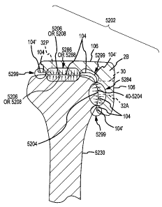
portions having patient-specific dimensions and configurations corresponding
to the actual dimensions and configurations of the targeted features 42 of the
patient's femur and tibia. The systems 4 and methods disclosed herein allow
for the efficient manufacture of arthroplasty jigs 2 customized for the
specific
bone features of a patient.
[0169] The jigs 2 and systems 4 and methods of producing such jigs are
illustrated herein in the context of knees and TKR surgery. However, those
skilled in the art will readily understand the jigs 2 and system 4 and methods
of producing such jigs can be readily adapted for use in the context of other
joints and joint replacement surgeries, e.g., elbows, shoulders, hips, etc.
Accordingly, the disclosure contained herein regarding the jigs 2 and systems
4 and methods of producing such jigs should not be considered as being
limited to knees and TKR surgery, but should be considered as encompassing
all types of joint surgeries.
[0170] c. Defining a 3D Surface Model of an Arthroplasty Target Area of a
Femur Lower End for Use as a Surface of an Interior Portion of a Femur
Arthroplasty Cutting Jig.
[0171] For a discussion of a method of generating a 3D model 40 of a target
area 42 of a damaged lower end 204 of a patient's femur 18, reference is
made to FIGS. 2A-2G. FIG. 2A is an anterior-posterior ("AP") image slice 208
of the damaged lower or knee joint end 204 of the patient's femur 18, wherein
the image slice 208 includes an open-loop contour line segment 210
corresponding to the target area 42 of the damaged lower end 204. FIG. 2B
is a plurality of image slices (16-1, 16-1, 16-2, ...16-n) with their
respective
open-loop contour line segments (210-1, 210-2, ... 210-n), the open-loop
contour line segments 210 being accumulated to generate the 3D model 40 of
the target area 42. FIG. 2C is a 3D model 40 of the target area 42 of the
CA 02730947 2011-01-14
WO 2010/011590
PCT/US2009/051109
32
damaged lower end 204 as generated using the open-loop contour line
segments (16-1, 16-2, ... 16-n) depicted in FIG. 2B. FIGS. 2D-2F are
respectively similar to FIGS. 2A-2C, except FIGS. 2D-2F pertain to a closed-
loop contour line as opposed to an open-loop contour line. FIG. 2G is a flow
chart illustrating an overview of the method of producing a femur jig 2A.
[0172]As can be understood from FIGS. 1A, 1B and 2A, the imager 8 is used
to generate a 2D image slice 16 of the damaged lower or knee joint end 204
of the patient's femur 18. As depicted in FIG. 2A, the 2D image 16 may be an
AP view of the femur 18. Depending on whether the imager 8 is a MRI or CT
imager, the image slice 16 will be a MRI or CT slice. The damaged lower end
204 includes the posterior condyle 212, an anterior femur shaft surface 214,
and an area of interest or targeted area 42 that extends from the posterior
condyle 212 to the anterior femur shaft surface 214. The targeted area 42 of
the femur lower end may be the articulating contact surfaces of the femur
lower end that contact corresponding articulating contact surfaces of the
tibia
upper or knee joint end.
[0173]As shown in FIG. 2A, the image slice 16 may depict the cancellous
bone 216, the cortical bone 218 surrounding the cancellous bone, and the
articular cartilage lining portions of the cortical bone 218. The contour line
210 may extend along the targeted area 42 and immediately adjacent the
cortical bone and cartilage to outline the contour of the targeted area 42 of
the
femur lower end 204. The contour line 210 extends along the targeted area
42 starting at point A on the posterior condyle 212 and ending at point B on
the anterior femur shaft surface 214.
[0174] In one embodiment, as indicated in FIG. 2A, the contour line 210
extends along the targeted area 42, but not along the rest of the surface of
the
femur lower end 204. As a result, the contour line 210 forms an open-loop
that, as will be discussed with respect to FIGS. 2B and 2C, can be used to
form an open-loop region or 3D computer model 40, which is discussed with
respect to [block 140] of FIG. 1D and closely matches the 3D surface of the
targeted area 42 of the femur lower end. Thus, in one embodiment, the
contour line is an open-loop and does not outline the entire cortical bone
CA 02730947 2011-01-14
WO 2010/011590
PCT/US2009/051109
33
surface of the femur lower end 204. Also, in one embodiment, the open-loop
process is used to form from the 3D images 16 a 3D surface model 36 that
generally takes the place of the arthritic model 36 discussed with respect to
[blocks 125-140] of FIG. 1D and which is used to create the surface model 40
used in the creation of the "jig data" 46 discussed with respect to [blocks
145-
150] of FIG. 1E.
[0175] In one embodiment and in contrast to the open-loop contour line 210
depicted in FIGS. 2A and 2B, the contour line is a closed-loop contour line
210' that outlines the entire cortical bone surface of the femur lower end and
results in a closed-loop area, as depicted in FIG. 2D. The closed-loop contour
lines 210'-2, ... 210'-n of each image slice 16-1, ... 16-n are combined, as
indicated in FIG. 2E. A closed-loop area may require the analysis of the
entire surface region of the femur lower end 204 and result in the formation
of
a 3D model of the entire femur lower end 204 as illustrated in FIG. 2F. Thus,
the 3D surface model resulting from the closed-loop process ends up having
in common much, if not all, the surface of the 3D arthritic model 36. In one
embodiment, the closed-loop process may result in a 3D volumetric
anatomical joint solid model from the 2D images 16 via applying mathematical
algorithms. U.S. Patent 5,682, 886, which was filed December 26, 1995 and
is incorporated by reference in its entirety herein, applies a snake algorithm
forming a continuous boundary or closed-loop. After the femur has been
outlined, a modeling process is used to create the 3D surface model, for
example, through a Bezier patches method. Other 3D modeling processes,
e.g., commercially-available 3D construction software as listed in other parts
of this Detailed Description, are applicable to 3D surface model generation
for
closed-loop, volumetric solid modeling.
[0176] In one embodiment, the closed-loop process is used to form from the
3D images 16 a 3D volumetric solid model 36 that is essentially the same as
the arthritic model 36 discussed with respect to [blocks 125-140] of FIG. 1D.
The 3D volumetric solid model 36 is used to create the surface model 40 used
in the creation of the "jig data" 46 discussed with respect to [blocks 145-
1501
of FIG. 1E.
CA 02730947 2011-01-14
WO 2010/011590
PCT/US2009/051109
34
[0177]The formation of a 3D volumetric solid model of the entire femur lower
end employs a process that may be much more memory and time intensive
than using an open-loop contour line to create a 3D model of the targeted
area 42 of the femur lower end. Accordingly, although the closed-loop
methodology may be utilized for the systems and methods disclosed herein,
for at least some embodiments, the open-loop methodology may be preferred
over the closed-loop methodology.
[0178]An example of a closed-loop methodology is disclosed in U.S. Patent
Application 11/641,569 to Park, which is entitled "Improved Total Joint
Arthroplasty System" and was filed January 19, 2007. This application is
incorporated by reference in its entirety into this Detailed Description.
[0179]As can be understood from FIGS. 2B and 2G, the imager 8 generates
a plurality of image slices (16-1, 16-2 ... 16-n) via repetitive imaging
operations [block 1000]. Each image slice 16 has an open-loop contour line
(210-1, 210-2 ... 210-n) extending along the targeted region 42 in a manner
as discussed with respect to FIG. 2A [block 1005]. In one embodiment, each
image slice is a two-millimeter 2D image slice 16. The system 4 compiles the
plurality of 2D image slices (16-1, 16-2 ... 16-n) and, more specifically, the
plurality of open-loop contour lines (210-1, 210-2, ... 210-n) into the 3D
femur
surface computer model 40 depicted in FIG. 2C [block 1010]. This process
regarding the generation of the surface model 40 is also discussed in the
overview section with respect to [blocks 100-105] of FIG. 1B and [blocks 130-
140] of FIG. 1D. A similar process may be employed with respect to the
closed-loop contour lines depicted in FIGS. 2D-2F.
[0180]As can be understood from FIG. 2C, the 3D femur surface computer
model 40 is a 3D computer representation of the targeted region 42 of the
femur lower end. In one embodiment, the 3D representation of the targeted
region 42 is a 3D representation of the articulated tibia contact surfaces of
the
femur distal end. As the open-loop generated 3D model 40 is a surface
model of the relevant tibia contacting portions of the femur lower end, as
opposed to a 3D model of the entire surface of the femur lower end as would
CA 02730947 2011-01-14
WO 2010/011590
PCT/US2009/051109
be a result of a closed-loop contour line, the open-loop generated 3D model
is less time and memory intensive to generate.
[0181]In one embodiment, the open-loop generated 3D model 40 is a surface
model of the tibia facing end face of the femur lower end, as opposed a 3D
model of the entire surface of the femur lower end. The 3D model 40 can be
used to identify the area of interest or targeted region 42, which, as
previously
stated, may be the relevant tibia contacting portions of the femur lower end.
Again, the open-loop generated 3D model 40 is less time and memory
intensive to generate as compared to a 3D model of the entire surface of the
femur distal end, as would be generated by a closed-loop contour line. Thus,
for at least some versions of the embodiments disclosed herein, the open-
loop contour line methodology is preferred over the closed-loop contour line
methodology. However, the system 4 and method disclosed herein may
employ either the open-loop or closed-loop methodology and should not be
limited to one or the other.
[0182]Regardless of whether the 3D model 40 is a surface model of the
targeted region 42 (i.e., a 3D surface model generated from an open-loop
process and acting as the arthritic model 22) or the entire tibia facing end
face
of the femur lower end (i.e., a 3D volumetric solid model generated from a
closed-loop process and acting as the arthritic model 22), the data pertaining
to the contour lines 210 can be converted into the 3D contour computer model
40 via the surface rendering techniques disclosed in any of the
aforementioned U.S. patent applications to Park. For example, surface
rending techniques employed include point-to-point mapping, surface normal
vector mapping, local surface mapping, and global surface mapping
techniques. Depending on the situation, one or a combination of mapping
techniques can be employed.
[0183]In one embodiment, the generation of the 3D model 40 depicted in FIG.
2C may be formed by using the image slices 16 to determine location
coordinate values of each of a sequence of spaced apart surface points in the
open-loop region of FIG. 2B. A mathematical model may then be used to
estimate or compute the 3D model 40 in FIG. 2C. Examples of other medical
CA 02730947 2011-01-14
WO 2010/011590
PCT/US2009/051109
36
imaging computer programs that may be used include, but are not limited to:
Analyze from AnalyzeDirect, Inc. of Overland Park, KS; open-source software
such as Paraview of Kitware, Inc.; Insight Toolkit ("ITK") available at
www.itk.org; 3D Slicer available at www.slicer.org; and Mimics from
Materialise of Ann Arbor, MI.
[0184] Alternatively or additionally to the aforementioned systems for
generating the 3D model 40 depicted in FIG. 2C, other systems for generating
the 3D model 40 of FIG. 2C include the surface rendering techniques of the
Non-Uniform Rational B-spline ("NURB") program or the Bezier program.
Each of these programs may be employed to generate the 3D contour model
40 from the plurality of contour lines 210.
[0185] In one embodiment, the NURB surface modeling technique is applied
to the plurality of image slices 16 and, more specifically, the plurality of
open-
loop contour lines 210 of FIG. 2B. The NURB software generates a 3D model
40 as depicted in FIG. 2C, wherein the 3D model 40 has areas of interest or
targeted regions 42 that contain both a mesh and its control points. For
example, see Ervin et al., Landscape Modeling, McGraw-Hill, 2001, which is
hereby incorporated by reference in its entirety into this Detailed
Description.
[0186] In one embodiment, the NURB surface modeling technique employs
kl k2
E E wo, AP(i, j)b,(s)b,(t)
G(s,t) - I kl k2
E E W(i,j)b,(s)b.,(t)
the following surface equation: 1=0 j=0 , wherein
P(i,j) represents a matrix of vertices with nrows = (k1+1) and ncols = (k2+1),
W(ij) represents a matrix of vertex weights of one per vertex point, b(s)
represents a row-direction basis or blending of polynomial functions of degree
Ml, WO represents a column-direction basis or blending polynomial functions
of degree M2, s represents a parameter array of row-direction knots, and t
represents a parameter array of column-direction knots.
[0187] In one embodiment, the Bezier surface modeling technique employs
the Bezier equation (1972, by Pierre Bezier) to generate a 3D model 40 as
depicted in FIG. 2C, wherein the model 40 has areas of interest or targeted
CA 02730947 2011-01-14
WO 2010/011590
PCT/US2009/051109
37
regions 42. A given Bezier surface of order (n, m) is defined by a set of
(n + 1)(m + 1) control points kid. It maps the unit square into a smooth-
continuous surface embedded within a space of the same dimensionality as
(k1,1). For example, if k are all points in a four-dimensional space, then the
surface will be within a four-dimensional space. This relationship holds true
for a one-dimensional space, a two-dimensional space, a fifty-dimensional
space, etc.
[0188]A two-dimensional Bezier surface can be defined as a parametric
surface where the position of a point p as a function of the parametric
ri. m
p(u, v) = E E Br (u) Br(v) ki,i
coordinates u, v is given by: i=o i=a evaluated
BliN = (7) ui(1 ¨ uri
z
over the unit square, where is a Bernstein
( n!
polynomial and 9.12) ¨ 1! * (72 ¨ 4)1 is the binomial coefficient. See Grune
et
al, On Numerical Algorithm and Interactive Visualization for Optimal Control
Problems, Journal of Computation and Visualization in Science, Vol. 1, No. 4,
July 1999, which is hereby incorporated by reference in its entirety into this
Detailed Description.
[0189]Various other surface rendering techniques are disclosed in other
references. For example, see the surface rendering techniques disclosed in
the following publications: Lorensen et al., Marching Cubes: A high
Resolution 3d Surface Construction Algorithm, Computer Graphics, 21-3: 163-
169, 1987; Farin et al., NURB Curves & Surfaces: From Projective Geometry
to Practical Use, Wellesley, 1995; Kumar et al, Robust Incremental Polygon
Triangulation for Surface Rendering, WSCG, 2000; Fleischer et al., Accurate
Polygon Scan Conversion Using Half-Open Intervals, Graphics Gems III, p.
362-365, code: p. 599-605, 1992; Foley et al., Computer Graphics: Principles
and Practice, Addison Wesley, 1990; Glassner, Principles of Digital Image
Synthesis, Morgan Kaufmann, 1995, all of which are hereby incorporated by
reference in their entireties into this Detailed Description.
CA 02730947 2011-01-14
WO 2010/011590
PCT/US2009/051109
38
[01901d. Selecting a Jig Blank Most Similar in Size and/or Configuration
to the Size of the Patient's Femur Lower End.
[0191]As mentioned above, an arthroplasty jig 2, such as a femoral jig 2A
includes an interior portion 100 and an exterior portion 102. The femoral jig
2A is formed from a femur jig blank 50A, which, in one embodiment, is
selected from a finite number of femur jig blank sizes. The selection of the
femur jig blank 50A is based on a comparison of the dimensions of the
patient's femur lower end 204 to the dimensions and/or configurations of the
various sizes of femur jig blanks 50A to select the femur jig blank 50A most
closely resembling the patient's femur lower end 204 with respect to size
and/or configuration. This selected femur jig blank 50A has an outer or
exterior side or surface 232 that forms the exterior portion 232 of the femur
jig
2A. The 3D surface computer model 40 discussed with respect to the
immediately preceding section of this Detail Description is used to define a
3D
surface 40 into the interior side 230 of computer model of a femur jig blank
50A. Furthermore, in some embodiments, the overestimation of the
procedure described below may be used to adjust the 3D surface model 40.
[0192] By selecting a femur jig blank 50A with an exterior portion 232 close
in
size to the patient's lower femur end 204, the potential for an accurate fit
between the interior portion 230 and the patient's femur is increased. Also,
the amount of material that needs to be machined or otherwise removed from
the jig blank 50A is reduced, thereby reducing material waste and
manufacturing time.
[0193] For a discussion of a method of selecting a jig blank 50 most closely
corresponding to the size and/or configuration of the patient's lower femur
end, reference is first made to FIGS. 3-4B. FIG. 3A is a top perspective view
of a left femoral cutting jig blank 50AL having predetermined dimensions.
FIG. 3B is a bottom perspective view of the jig blank 50AL depicted in FIG.
3A. FIG. 3C is plan view of an exterior side or portion 232 of the jig blank
50AL depicted in FIG. 3A. FIG. 4A is a plurality of available sizes of left
femur
jig blanks 50AL, each depicted in the same view as shown in FIG. 3C. FIG.
CA 02730947 2011-01-14
WO 2010/011590
PCT/US2009/051109
39
4B is a plurality of available sizes of right femur jig blanks 50AR, each
depicted in the same view as shown in FIG. 3C.
[0194]A common jig blank 50, such as the left jig blank 50AL depicted in
FIGS. 3A-3C and intended for creation of a left femur jig that can be used
with
a patient's left femur, may include a posterior edge 240, an anterior edge
242,
a lateral edge 244, a medial edge 246, a lateral condyle portion 248, a medial
condyle portion 250, the exterior side 232 and the interior side 230. The jig
blank 50AL of FIGS. 3A-3C may be any one of a number of left femur jig
blanks 50AL available in a limited number of standard sizes. For example,
the jig blank 50AL of FIGS. 3A-3C may be an i-th left femur jig blank, where i
= 1, 2, 3, 4, .... m and m represents the maximum number of left femur jig
blank sizes.
[0195]As indicated in FIG. 3C, the anterior-posterior extent JAi of the jig
blank
50AL is measured from the anterior edge 242 to the posterior edge 240 of the
jig blank 50AL. The medial-lateral extent JMi of the jig blank 50AL is
measured from the lateral edge 244 to the medial edge 246 of the jig blank
50AL.
[0196]As can be understood from FIG. 4A, a limited number of left femur jig
blank sizes may be available for selection as the left femur jig blank size to
be
machined into the left femur cutting jig 2A. For example, in one embodiment,
there are nine sizes (m = 9) of left femur jig blanks 50AL available. As can
be
understood from FIG. 3C, each femur jig blank 50AL has an anterior-
posterior/medial-lateral aspect ratio defined as JAi to JMi (e.g., "JAi/JMi"
aspect ratio). Thus, as can be understood from FIG. 4A, jig blank 50AL-1 has
an aspect ratio defined as "JAi/JMi", jig blank 50AL-2 has an aspect ratio
defined as "JA2/JM2", jig blank 50AL-3 has an aspect ratio defined as
"JA3/JM3", jig blank 50AL-4 has an aspect ratio defined as "JA4/JM4", jig
blank
50AL-5 has an aspect ratio defined as "JA5/JM5", jig blank 50AL-6 has an
aspect ratio defined as "JA8/JM8", jig blank 50AL-7 has an aspect ratio
defined
as "JA7/JM7", jig blank 50AL-8 has an aspect ratio defined as "JA8/JM8", and
jig blank 50AL-9 has an aspect ratio defined as "JA9/JM9".
CA 02730947 2011-01-14
WO 2010/011590
PCT/US2009/051109
[0197] The jig blank aspect ratio is utilized to design left femur jigs 2A
dimensioned specific to the patient's left femur features. In one embodiment,
the jig blank aspect ratio can be the exterior dimensions of the left femur
jig
2A. In another embodiment, the jig blank aspect ratio can apply to the left
femur jig fabrication procedure for selecting the left jig blank 50AL having
parameters close to the dimensions of the desired left femur jig 2A. This
embodiment can improve the cost efficiency of the left femur jig fabrication
process because it reduces the amount of machining required to create the
desired jig 2 from the selected jig blank 50.
[0198] In FIG. 4A, the N-1 direction represents increasing jig aspect ratios
moving from jig 50AL-3 to jig 50AL-2 to jig 50AL-1, where "JA3/JM3" <
"JA2/JM2" < "JAi/JMi". The increasing ratios of the jigs 50AL represent the
corresponding increment of JAi values, where the jigs' JMi values remain the
same. In other words, since JA3 < JA2 < JAi, and JM3= JM2= JMi, then
"JA3/JM3" < "JA2/JM2" < "JAi/JMi". One example of the increment level can
be an increase from 5% to 20%.
[0199] The same rationale applies to the N-2 direction and the N-3 direction.
For example, the N-2 direction represents increasing jig aspect ratios from
jig
50AL-6 to jig 50AL-5 to jig 50AL-4, where "JA4/JM4" < "JA5/JM5" < "JA6/JM6".
The increasing ratios of the jigs 50AL represent the corresponding increment
of JAi values, where the JMi values remain the same. The N-3 direction
represents increasing jig aspect ratios from jig 50AL-9 to jig 50AL-8 to jig
50AL-7, where "JA7/JM7" < "JA8/JM8" < "JA9/JM9". The increasing ratios of the
jigs 50AL represent the corresponding increment of JAi values, where the JMi
values remain the same.
[0200] As can be understood from the plot 300 depicted in FIG. 7 and
discussed later in this Detailed Discussion, the E-1 direction corresponds to
the sloped line joining Group 1, Group 4 and Group 7. Similarly, the E-2
direction corresponds to the sloped line joining Group 2, Group 5 and Group
8. Also, the E-3 direction corresponds to the sloped line joining Group 3,
Group 6 and Group 9.
CA 02730947 2011-01-14
WO 2010/011590
PCT/US2009/051109
41
[0201]As indicated in FIG. 4A, along direction E-2, the jig aspect ratios
remain the same among jigs 50AL-2, 50AL-5 and jig 50AL-8, where "JA2 /JM2"
= "JA5 /JM5" = "JA8 /JM8". However, comparing to jig 50AL-2, jig 50AL-5 is
dimensioned larger and longer than jig 50AL-2. This is because the JA5 value
for jig 50AL-5 increases proportionally with the increment of its JM5 value in
certain degrees in all X, Y, and Z-axis directions. In a similar fashion, jig
50AL-8 is dimensioned larger and longer than jig 50AL-5 because the JA5
increases proportionally with the increment of its JM8 value in certain
degrees
in all X, Y, and Z-axis directions. One example of the increment can be an
increase from 5% to 20%.
[0202] The same rationale applies to directions E-1 and E-3. For example, in
E-3 direction the jig ratios remain the same among the jigs 50AL-3, 50AL-6
and jig 50AL-9. Compared to jig 50AL-3, jig 50AL-6 is dimensioned bigger
and longer because both JM8 and JA8 values of jig 50AL-6 increase
proportionally in all X, Y, and Z-axis directions. Compared to jig 50AL-6, jig
50AL-9 is dimensioned bigger and longer because both JM9 and JA9 values of
jig 50AL-9 increase proportionally in all X, Y, and Z-axis.
[0203]As can be understood from FIG. 4B, a limited number of right femur jig
blank sizes may be available for selection as the right femur jig blank size
to
be machined into the right femur cutting jig 2A. For example, in one
embodiment, there are nine sizes (m = 9) of right femur jig blanks 50AR
available. As can be understood from FIG. 3, each femur jig blank SOAR has
an anterior-posterior/medial-lateral aspect ratio defined as JAi to JMi (e.g.,
"JAi/JMi" aspect ratio). Thus, as can be understood from FIG. 4B, jig blank
SOAR-1 has an aspect ratio defined as "JAi/JMi", jig blank SOAR-2 has an
aspect ratio defined as "JA2/JM2", jig blank 50AR-3 has an aspect ratio
defined as "JA3/JM3", jig blank 50AR-4 has an aspect ratio defined as
"JA4/JM4", jig blank 50AR-5 has an aspect ratio defined as "JA5/JM5", jig
blank
50AR-6 has an aspect ratio defined as "JA8/JM8", jig blank 50AR-7 has an
aspect ratio defined as "JA7/JM7", jig blank 50AR-8 has an aspect ratio
defined as "JA8/JM8", and jig blank SOAR-9 has an aspect ratio defined as
"JA9/JM9".
CA 02730947 2011-01-14
WO 2010/011590
PCT/US2009/051109
42
[0204] The jig blank aspect ratio may be utilized to design right femur jigs
2A
dimensioned specific to the patient's right femur features. In one
embodiment, the jig blank aspect ratio can be the exterior dimensions of the
right femur jig 2A. In another embodiment, the jig blank aspect ratio can
apply
to the right femur jig fabrication procedure for selecting the right jig blank
50AR having parameters close to the dimensions of the desired right femur jig
2A. This embodiment can improve the cost efficiency of the right femur jig
fabrication process because it reduces the amount of machining required to
create the desired jig 2 from the selected jig blank 50.
[0205] In FIG. 4B, the N-1 direction represents increasing jig aspect ratios
moving from jig 50AR-3 to jig 50AR-2 to jig 50AR-1, where "JA3/JM3" <
"JA2/JM2" < "JAi/JMi". The increasing ratios of the jigs 50AR represent the
corresponding increment of JAi values, where the jigs' JMi values remain the
same. In other words, since JA3 < JA2 < JAi, and JM3= JM2= JMi, then
"JA3/JM3" < "JA2/JM2" < "JAi/JMi". One example of the increment level can
be an increase from 5% to 20%.
[0206] The same rationale applies to the N-2 direction and the N-3 direction.
For example, the N-2 direction represents increasing jig aspect ratios from
jig
50AR-6 to jig 50AR-5 to jig 50AR-4, where "JA4/JM4" < "JA5/JM5" < "JA6/JM6".
The increasing ratios of the jigs 50AR represent the corresponding increment
of JAi values, where the JMi values remain the same. The N-3 direction
represents increasing jig aspect ratios from jig 50AR-9 to jig 50AR-8 to jig
50AR-7, where "JA7/JM7" < "JA5/JM8" < "JA9/JM9". The increasing ratios of
the jigs 50AR represent the corresponding increment of JAi values, where the
JMi values remain the same.
[0207] As indicated in FIG. 4B, along direction E-2, the jig aspect ratios
remain the same among jigs 50AR-2, 50AR-5 and jig 50AR-8, where "JA2
/JM2" = "JA5 /JM5" = "JA5 /JM5". However, comparing to jig 50AR-2, jig 50AR-
is dimensioned larger and longer than jig 50AR-2. This is because the JA5
value for jig 50AR-5 increases proportionally with the increment of its JM5
value in certain degrees in all X, Y, and Z-axis directions. In a similar
fashion,
jig 50AR-8 is dimensioned larger and longer than jig 50AR-5 because the JA8
CA 02730947 2011-01-14
WO 2010/011590
PCT/US2009/051109
43
increases proportionally with the increment of its JM8 value in certain
degrees
in all X, Y, and Z-axis directions. One example of the increment can be an
increase from 5% to 20%.
[0208] The same rationale applies to directions E-1 and E-3. For example, in
E-3 direction the jig ratios remain the same among the jigs 50AR-3, 50AR-6
and jig 50AR-9. Compared to jig 50AR-3, jig 50AR-6 is dimensioned bigger
and longer because both JM6and JA8 values of jig 50AR-6 increase
proportionally in all X, Y, and Z-axis directions. Compared to jig 50AR-6, jig
50AR-9 is dimensioned bigger and longer because both JM9 and JA9 values of
jig 50AR-9 increase proportionally in all X, Y, and Z-axis.
[0209] The dimensions of the lower or knee joint forming end 204 of the
patient's femur 18 can be determined by analyzing the 3D surface model 40
or 3D arthritic model 36 in a manner similar to those discussed with respect
to
the jig blanks 50. For example, as depicted in FIG. 5, which is an axial view
of the 3D surface model 40 or arthritic model 36 of the patient's left femur
18
as viewed in a direction extending distal to proximal, the lower end 204 of
the
surface model 40 or arthritic model 36 may include an anterior edge 262, a
posterior edge 260, a medial edge 264, a lateral edge 266, a medial condyle
268, and a lateral condyle 270. The femur dimensions may be determined for
the bottom end face or tibia articulating surface 204 of the patient's femur
18
via analyzing the 3D surface model 40 of the 3D arthritic model 36. These
femur dimensions can then be utilized to configure femur jig dimensions and
select an appropriate femur jig.
[0210] As shown in FIG. 5, the anterior-posterior extent fAP of the lower end
204 of the patient's femur 18 (i.e., the lower end 204 of the surface model 40
of the arthritic model 36, whether formed via open or closed-loop analysis) is
the length measured from the anterior edge 262 of the femoral lateral groove
to the posterior edge 260 of the femoral lateral condyle 270. The medial-
lateral extent fML of the lower end 204 of the patient's femur 18 is the
length
measured from the medial edge 264 of the medial condyle 268 to the lateral
edge 266 of the lateral condyle 270.
CA 02730947 2011-01-14
WO 2010/011590
PCT/US2009/051109
44
[0211] In one embodiment, the anterior-posterior extent fAP and medial-lateral
extent fML of the femur lower end 204 can be used for an aspect ratio
fAP/fML of the femur lower end. The aspect ratios fAP/fML of a large number
(e.g., hundreds, thousands, tens of thousands, etc.) of patient knees can be
compiled and statistically analyzed to determine the most common aspect
ratios for jig blanks that would accommodate the greatest number of patient
knees. This information may then be used to determine which one, two,
three, etc. aspect ratios would be most likely to accommodate the greatest
number of patient knees.
[0212] The system 4 analyzes the lower ends 204 of the patient's femur 18 as
provided via the surface model 40 of the arthritic model 36 (whether the
arthritic model 36 is an 3D surface model generated via an open-loop or a 3D
volumetric solid model generated via a closed-loop process) to obtain data
regarding anterior-posterior extent fAP and medial-lateral extent fML of the
femur lower ends 204. As can be understood from FIG. 6, which depicts the
selected model jig blank 50AL of FIG. 3C superimposed on the model femur
lower end 204 of FIG. 5, the femur dimensional extents fAP, fML are
compared to the jig blank dimensional extents JAR, jML to determine which jig
blank model to select as the starting point for the machining process and the
exterior surface model for the jig model.
[0213]As shown in FIG. 6, a prospective left femoral jig blank 50AL is
superimposed to mate with the left femur lower end 204 of the patient's
anatomical model as represented by the surface model 40 or arthritic model
36. The jig blank 50AL covers most of medial condyle 268 and the lateral
condyle 270, leaving small exposed condyle regions including t1, t2, t3. The
medial medial-lateral condyle region t1 represents the region between the
medial edge 264 of the medial condyle 268 and the medial edge 246 of the jig
blank 50AL. The lateral medial-lateral condyle region t2 represents the region
between the lateral edge 266 of the lateral condyle 270 and the lateral edge
244 of the jig blank 50AL. The posterior anterior-posterior region t3
represents the condyle region between the posterior edge 260 of the lateral
condyle 270 and the posterior edge 240 of the jig blank 50AL.
CA 02730947 2011-01-14
WO 2010/011590
PCT/US2009/051109
[0214] The anterior edge 242 of the jig blank 50AL extends past the anterior
edge 262 of the left femur lower end 204 as indicated by anterior anterior-
posterior overhang t4. Specifically, the anterior anterior-posterior overhang
t4
represents the region between the anterior edge 262 of the lateral groove of
femur lower end 204 and the anterior edge 242 of the jig blank 50AL. By
obtaining and employing the femur anterior-posterior fAP data and the femur
medial-lateral fML data, the system 4 can size the femoral jig blank 50AL
according to the following formulas: as jFML = fML ¨ t1 ¨ t2 and jFAP = fAP ¨
t3 + t4, wherein jFML is the medial-lateral extent of the femur jig blank 50AL
and jFAP is the anterior-posterior extent of the femur jig blank 50AL. In one
embodiment, t1, t2, t3 and t4 will have the following ranges: 2mm ===t1 6mm,
2mm ===t2 .6mm; 2mm 12mm; and 15mm ...25mm. In another
embodiment, t1, t2, t3 and t4 will have the following values: t1= 3mm; t2 =
3mm; t3 = 6mm; and t4 = 20mm.
[0215] FIG. 7A is an example scatter plot 300 for selecting from a plurality
of
candidate jig blanks sizes a jig blank size appropriate for the lower end 204
of
the patient's femur 18. In one embodiment, the X-axis represents the
patient's femoral medial-lateral length fML in millimeters, and the Y-axis
represents the patient's femoral anterior-posterior length fAP in millimeters.
In
one embodiment, the plot is divided into a number of jig blank size groups,
where each group encompasses a region of the plot 300 and is associated
with specific parameters JMr, JAr of a specific candidate jig blank size.
[0216] In one embodiment, the example scatter plot 300 depicted in FIG. 7A
has nine jig blank size groups, each group pertaining to a single candidate
jig
blank size. However, depending on the embodiment, a scatter plot 300 may
have a greater or lesser number of jig blank size groups. The higher the
number of jig blank size groups, the higher the number of the candidate jig
blank sizes and the more dimension specific a selected candidate jig blank
size will be to the patient's knee features and the resulting jig 2. The more
dimension specific the selected candidate jig blank size, the lower the amount
of machining required to produce the desired jig 2 from the selected jig blank
50.
CA 02730947 2011-01-14
WO 2010/011590
PCT/US2009/051109
46
[0217] Conversely, the lower the number of jig blank size groups, the lower
the number of candidate jig blank sizes and the less dimension specific a
selected candidate jig blank size will be to the patient's knee features and
the
resulting jig 2. The less dimension specific the selected candidate jig blank
size, the higher the amount of machining required to produce the desired jig 2
from the selected jig blank 50, adding extra roughing during the jig
fabrication
procedure.
[0218] As can be understood from FIG. 7A, in one embodiment, the nine jig
blank size groups of the plot 300 have the parameters JMr, JAr as follows.
Group 1 has parameters JMi, JA1. JMi represents the medial-lateral extent of
the first femoral jig blank size, wherein JMi =70mm. JAi represents the
anterior-posterior extent of the first femoral jig blank size, wherein JAi =
70.5mm. Group 1 covers the patient's femur fML and fAP data wherein
55mm < fML < 70mm and 61MM < fAP < 70.5mm.
[0219] Group 2 has parameters JM2, JA2. JM2 represents the medial-lateral
extent of the second femoral jig blank size, wherein JM2= 70mm. JA2
represents the anterior-posterior extent of the second femoral jig blank size,
wherein JA2 = 61.5mm. Group 2 covers the patient's femur fML and fAP data
wherein 55mm < fML < 70mm and 52mm < fAP < 61.5mm.
[0220] Group 3 has parameters JM3, JA3. JM3 represents the medial-lateral
extent of the third femoral jig blank size, wherein JM3= 70mm. JA3 represents
the anterior-posterior extent of the third femoral jig blank size, wherein JA3
=
52mm. Group 3 covers the patient's femur fML and fAP data wherein 55mm
< fML < 70mm and 40mm < fAP < 52mm.
[0221] Group 4 has parameters JM4, JA4. JM4 represents the medial-lateral
extent of the fourth femoral jig blank size, wherein JM4= 85mm. JA4
represents the anterior-posterior extent of the fourth femoral jig blank size,
wherein JA4 = 72.5mm. Group 4 covers the patient's femur fML and fAP data
wherein 70mm < fML <85mm and 63.5mm < fAP < 72.5mm.
[0222] Group 5 has parameters JM5, JA5. JM5 represents the medial-lateral
extent of the fifth femoral jig blank size, wherein JM5= 85mm. JA5 represents
CA 02730947 2011-01-14
WO 2010/011590
PCT/US2009/051109
47
the anterior-posterior extent of the fifth femoral jig blank size, wherein
JA5=
63.5mm. Group 5 covers the patient's femur fML and fAP data wherein
70mm < fML < 85mm and 55mm < fAP < 63.5mm.
[0223] Group 6 has parameters JM6, JA6. JM6 represents the medial-lateral
extent of the sixth femoral jig blank size, wherein JM6= 85mm. JA6
represents the anterior-posterior extent of the sixth femoral jig blank size,
wherein JA6= 55mm. Group 6 covers the patient's femur fML and fAP data
wherein 70mm < fML < 85mm and 40mm < fAP < 55mm.
[0224] Group 7 has parameters JM7, JA7. JM7 represents the medial-lateral
extent of the seventh femoral jig blank size, wherein JM7 = 100mm. JA7
represents the anterior-posterior extent of the seventh femoral jig blank
size,
wherein JA7= 75nnm. Group 7 covers the patient's femur fML and fAP data
wherein 85mm < fML < 100mm and 65mm < fAP < 75mm.
[0225] Group 8 has parameters JM8, JA8. JM8 represents the medial-lateral
extent of the eighth femoral jig blank size, wherein JM8= 100mm. JA8
represents the anterior-posterior extent of the eighth femoral jig blank size,
wherein JA8= 65mm. Group 8 covers the patient's femur fML and fAP data
wherein 85mm < fML < 100mm and 57.5mm < fAP < 65mm.
[0226] Group 9 has parameters JM9, JA9. JM9 represents the medial-lateral
extent of the ninth femoral jig blank size, wherein JM9= 100mm. JA9
represents the anterior-posterior extent of the ninth femoral jig blank size,
wherein JA9= 57.5mm. Group 9 covers the patient's femur fML and fAP data
wherein 85mm < fML < 100mm and 40mm < fAP < 57.5mm.
[0227] As can be understood from FIG. 7B, which is a flow diagram illustrating
an embodiment of a process of selecting an appropriately sized jig blank,
bone anterior-posterior and medial-lateral extents fAP, fML are determined for
the lower end 204 of the surface model 40 of the arthritic model 36 [block
2000]. The bone extents fAP, fML of the lower end 204 are mathematically
modified according to the above discussed jFML and jFAP formulas to arrive
at the minimum femur jig blank anterior-posterior extent jFAP and medial-
lateral extent jFML [block 20101. The mathematically modified bone extents
CA 02730947 2011-01-14
WO 2010/011590
PCT/US2009/051109
48
fAP, fML or, more specifically, the minimum femur jig blank anterior-posterior
and medial-lateral extents jFAP, jFML are referenced against the jig blank
dimensions in the plot 300 of FIG. 7A [block 2020]. The plot 300 may
graphically represent the extents of candidate femur jig blanks forming a jig
blank library. The femur jig blank 50A is selected to be the jig blank size
having the smallest extents that are still sufficiently large to accommodate
the
minimum femur jig blank anterior-posterior and medial-lateral extents JFAP,
jFML [block 2030].
[0228] In one embodiment, the exterior of the selected jig blank size is used
for the exterior surface model of the jig model, as discussed below. In one
embodiment, the selected jig blank size corresponds to an actual jig blank
that
is placed in the CNC machine and milled down to the minimum femur jig blank
anterior-posterior and medial-lateral extents jFAP, jFML to machine or
otherwise form the exterior surface of the femur jig 2A.
[0229] The method outlined in FIG. 7B and in reference to the plot 300 of FIG.
7A can be further understood from the following example. As measured in
FIG. 6 with respect to the lower end 204 of the patient's femur 18, the
extents
of the patient's femur are as follows: fML = 79.2mm and fAP = 54.5mm [block
2000]. As previously mentioned, the lower end 204 may be part of the
surface model 40 of the arthritic model 36. Once the fML and fAP
measurements are determined from the lower end 204, the corresponding jig
jFML data and jig jFAP data can be determined via the above-described jFML
and jFAP formulas: jFML = fML ¨ t1 ¨ t2, wherein t1 = 3mm and t2= 3mm;
and jFAP = fAP ¨ t3 + t4, wherein t3 = 6mm and t4= 20mm [block 20101. The
result of the jFML and jFAP formulas is jFML = 73.2mm and jFAP = 68.5mm.
[0230] As can be understood from the plot 300 of FIG. 7, the determined jig
data (i.e., jFML = 73.2mm and jFAP = 68.5mm) falls in Group 4 of the plot
300. Group 4 has the predetermined femur jig blank parameters (JM4, JA4) of
JM4 = 85mm and JA4 = 72.5mm. These predetermined femur jig blank
parameters are the smallest of the various groups that are still sufficiently
large to meet the minimum femur blank extents jFAP, jFML [block 2020].
These predetermined femur jig blank parameters (JM4 = 85mm and JA4 =
CA 02730947 2011-01-14
WO 2010/011590
PCT/US2009/051109
49
72.5mm) may be selected as the appropriate femur jig blank size [block
2030].
[0231] In one embodiment, the predetermined femur jig blank parameters
(85mm, 72.5mm) can apply to the femur exterior jig dimensions as shown in
FIG. 3C. In other words, the jig blank exterior is used for the jig model
exterior as discussed with respect to FIGS. 8A-9C. Thus, the exterior of the
femur jig blank 50A undergoes no machining, and the unmodified exterior of
the jig blank 50A with its predetermined jig blank parameters (85mm,
72.5mm) serves as the exterior of the finished femur jig 2A.
[0232] In another embodiment, the femur jig blank parameters (85mm,
72.5mm) can be selected for jig fabrication in the machining process. Thus, a
femur jig blank 50A having predetermined parameters (85mm, 72.5mm) is
provided to the machining process such that the exterior of the femur jig
blank
50A will be machined from its predetermined parameters (85mm, 72.5mm)
down to the desired femur jig parameters (73.2, 68.5mm) to create the
finished exterior of the femur jig 2A. As the predetermined parameters
(85mm, 72.5mm) are selected to be relatively close to the desired femur jig
parameters (73.2, 68.5mm), machining time and material waste are reduced.
[0233] While it may be advantageous to employ the above-described jig blank
selection method to minimize material waste and machining time, in some
embodiments, a jig blank will simply be provided that is sufficiently large to
be
applicable to all patient bone extents fAP, fML. Such a jig blank is then
machined down to the desired jig blank extents jFAP, jFML, which serve as
the exterior surface of the finished jig 2A.
[0234] In one embodiment, the number of candidate jig blank size groups
represented in the plot 300 is a function of the number of jig blank sizes
offered by a jig blank manufacturer. For example, a first plot 300 may pertain
only to jig blanks manufactured by company A, which offers nine jig blank
sizes. Accordingly, the plot 300 has nine jig blank size groups. A second plot
300 may pertain only to jig blanks manufactured by company B, which offers
twelve jig blank size groups. Accordingly, the second plot 300 has twelve jig
blank size groups.
CA 02730947 2011-01-14
WO 2010/011590
PCT/US2009/051109
[0235] A plurality of candidate jig blank sizes exist, for example, in a jig
blank
library as represented by the plot 300 of FIG. 7B. While each candidate jig
blank may have a unique combination of anterior-posterior and medial-lateral
dimension sizes, in some embodiments, two or more of the candidate jig
blanks may share a common aspect ratio jAP/jML or configuration. The
candidate jig blanks of the library may be grouped along sloped lines of the
plot 300 according to their aspect ratios jAP/jML.
[0236] In one embodiment, the jig blank aspect ratio jAP/jML may be used to
take a workable jig blank configuration and size it up or down to fit larger
or
smaller individuals.
[0237] As can be understood from FIG. 7A, a series of 98 OA patients having
knee disorders were entered into the plot 300 as part of a femur jig design
study. Each patient's femur fAP and fML data was measured and modified
via the above-described jFML and jFAP formulas to arrive at the patient's jig
blank data (jFML, jFAP). The patient's jig blank data was then entered into
the plot 300 as a point. As can be understood from FIG. 7A, no patient point
lies outside the parameters of an available group. Such a process can be
used to establish group parameters and the number of needed groups.
[0238] In one embodiment, the selected jig blank parameters can be the
femoral jig exterior dimensions that are specific to patient's knee features.
In
another embodiment, the selected jig blank parameters can be chosen during
fabrication process.
[02391e. Formation of 3D Femoral Jig Model.
[0240] For a discussion of an embodiment of a method of generating a 3D
femur jig model 346 generally corresponding to the "integrated jig data" 48
discussed with respect to [block 150] of FIG. 1E, reference is made to FIGS.
3A-3C, FIGS. 8A-8B, FIGS. 9A-9C and FIG. 10A-10B. FIGS. 3A-3C are
various views of a femur jig blank 50A. FIGS. 8A-8B are, respectively,
exterior and interior perspective views of a femur jig blank exterior surface
model 232M. FIGS. 9A and 9B are exterior perspective views of the jig blank
exterior model 232M and bone surface model 40 being combined, and FIG.
CA 02730947 2011-01-14
WO 2010/011590
PCT/US2009/051109
51
9C is a cross section through the combined models 232M, 40 as taken along
section line 9C-9C in FIG. 9B. FIGS. 10A and 10B are, respectively, exterior
and interior perspective views of the resulting femur jig model 346 after
having
"saw cut and drill hole data" 44 integrated into the jig model 346 to become
an
integrated or complete jig model 348 generally corresponding to the
"integrated jig data" 48 discussed with respect to [block 150] of FIG. 1E.
[0241]As can be understood from FIGS. 3A-3C, the jig blank 50A, which has
selected predetermined dimensions as discussed with respect to FIG. 7,
includes an interior surface 230 and an exterior surface 232. The exterior
surface model 232M depicted in FIGS. 8A and 8B is extracted or otherwise
created from the exterior surface 232 of the jig blank model 50A. Thus, the
exterior surface model 232M is based on the jig blank aspect ratio of the
femur jig blank 50A selected as discussed with respect to FIG. 7 and is
dimensioned specific to the patient's knee features. The femoral jig surface
model 232M can be extracted or otherwise generated from the jig blank model
50A of FIGS. 3A-3C by employing any of the computer surface rendering
techniques described above.
[0242]As can be understood from FIGS. 9A-9C, the exterior surface model
232M is combined with the femur surface model 40 to respectively form the
exterior and interior surfaces of the femur jig model 346. The femur surface
model 40 represents the interior or mating surface of the femur jig 2A and
corresponds to the femur arthroplasty target area 42. Thus, the model 40
allows the resulting femur jig 2A to be indexed to the arthroplasty target
area
42 of the patient's femur 18 such that the resulting femur jig 2A will
matingly
receive the arthroplasty target area 42 during the arthroplasty procedure. The
two surface models 232M, 40 combine to provide a patient-specific jig model
346 for manufacturing the femur jig 2A. In some embodiments, this patient-
specific jig model 346 may include one or more areas of overestimation (as
described below) to accommodate for irregularities in the patient's bone
surface and/or limitations in jig manufacturing capabilities.
[0243]As can be understood from FIGS. 9B and 9C, once the models 232M,
40 are properly aligned, a gap will exist between the two models 232M, 40.
CA 02730947 2011-01-14
WO 2010/011590
PCT/US2009/051109
52
An image sewing method or image sewing tool is applied to the aligned
models 232M, 40 to join the two surface models together to form the 3D
computer generated jig model 346 of FIG. 9B into a single-piece, joined-
together, and filled-in jig model 346 similar in appearance to the integrated
jig
model 348 depicted in FIGS. 10A and 10B. In one embodiment, the jig model
346 may generally correspond to the description of the "jig data" 46 discussed
with respect [block 145] of FIG. 1E.
[0244] As can be understood from FIGS. 9B and 9C, the geometric gaps
between the two models 232M, 40, some of which are discussed below with
respect to thicknesses P1, P2 and P3, may provide certain space between the
two surface models 232M, 40 for slot width and length and drill bit length for
receiving and guiding cutting tools during TKA surgery. Because the resulting
femur jig model 348 depicted in FIGS. 10A and 10B may be a 3D volumetric
model generated from 3D surface models 232M, 40, a space or gap should
be established between the 3D surface models 232M, 40. This allows the
resulting 3D volumetric jig model 348 to be used to generate an actual
physical 3D volumetric femur jig 2.
[0245] In some embodiments, the image processing procedure may include a
model repair procedure for repairing the jig model 346 after alignment of the
two models 232M, 40. For example, various methods of the model repairing
include, but are not limit to, user-guided repair, crack identification and
filling,
and creating manifold connectivity, as described in: Nooruddin et al.,
Simplification and Repair of Polygonal Models Using Volumetric Techniques
(IEEE Transactions on Visualization and Computer Graphics, Vol.9, No.2,
April-June 2003); C. Erikson, Error Correction of a Large Architectural Model:
The Henderson County Courthouse (Technical Report TR95-013, Dept. of
Computer Science, Univ. of North Carolina at Chapel Hill, 1995); D.
Khorramabdi, A Walk through the Planned CS Building (Technical Report
UCB/CSD 91/652, Computer Science Dept., Univ. of California at Berkeley,
1991); Morvan et al., IVECS: An Interactive Virtual Environment for the
Correction of .STL files (Proc. Conf. Virtual Design, Aug. 1996); Bohn et al.,
A
Topology-Based Approach for Shell-Closure, Geometric Modeling for Product
CA 02730947 2011-01-14
WO 2010/011590
PCT/US2009/051109
53
Realization, (P.R. Wilson et al., pp. 297-319, North-Holland, 1993); Barequet
et al., Filling Gaps in the Boundary of a Polyhedron, Computer Aided
Geometric Design (vol. 12, no. 2, pp. 207-229, 1995); Barequet et al.,
Repairing CAD Models (Proc. IEEE Visualization '97, pp. 363-370, Oct. 1997);
and Gueziec et al., Converting Sets of Polygons to Manifold Surfaces by
Cutting and Stitching, (Proc. IEEE Visualization 1998, pp. 383-390, Oct.
1998). Each of these references is incorporated into this Detailed Description
in their entireties.
[0246]As can be understood from FIGS. 10A and 10B, the integrated jig
model 348 may include several features based on the surgeon's needs. For
example, the jig model 348 may include a slot feature 30 for receiving and
guiding a bone saw and drill holes 32 for receiving and guiding bone drill
bits.
As can be understood from FIGS. 9B and 9C, to provide sufficient structural
integrity to allow the resulting femur jig 2A to not buckle or deform during
the
arthroplasty procedure and to adequately support and guide the bone saw
and drill bits, the gap 350 between the models 232M, 40 may have the
following offsets P1, P2, and P3.
[0247]/Ns can be understood from FIGS. 9B-10B, in one embodiment,
thickness P1 extends along the length of the anterior drill holes 32A between
the models 232M, 40 and is for supporting and guiding a bone drill received
therein during the arthroplasty procedure. Thickness P1 may be at least
approximately four millimeters or at least approximately five millimeters
thick.
The diameter of the anterior drill holes 32A may be configured to receive a
cutting tool of at least one-third inches.
[0248] Thickness P2 extends along the length of a saw slot 30 between the
models 232M, 40 and is for supporting and guiding a bone saw received
therein during the arthroplasty procedure. Thickness P2 may be at least
approximately lOmm or at least 15mm thick.
[0249] Thickness P3 extends along the length of the posterior drill holes 32P
between the models 232M, 40 and is for supporting and guiding a bone drill
received therein during the arthroplasty procedure. Thickness P3 may be at
least approximately five millimeters or at least eight millimeters thick. The
CA 02730947 2011-01-14
WO 2010/011590
PCT/US2009/051109
54
diameter of the drill holes 32 may be configured to receive a cutting tool of
at
least one-third inches.
[0250]In addition to providing sufficiently long surfaces for guiding drill
bits or
saws received therein, the various thicknesses P1, P2, P3 are structurally
designed to enable the femur jig 2A to bear vigorous femur cutting, drilling
and reaming procedures during the TKR surgery.
[0251]As indicated in FIGS. 10A and 10B, the integrated jig model 348 may
include: feature 400 that matches the patient's distal portion of the medial
condyle cartilage; feature 402 that matches the patient's distal portion of
the
lateral condyle cartilage; projection 404 that can be configured as a contact
or
a hook and may securely engage the resulting jig 2A onto the patient's
anterior femoral joint surface during the TKR surgery; and the flat surface
406
that provides a blanked labeling area for listing information regarding the
patient, surgeon or/and the surgical procedure. Also, as discussed above, the
integrated jig model 348 may include the saw cut slot 30 and the drill holes
32. The inner portion or side 100 of the jig model 348 (and the resulting
femur
jig 2A) is the femur surface model 40, which will matingly receive the
arthroplasty target area 42 of the patient's femur 18 during the arthroplasty
procedure. In some embodiments, the overestimation of the procedure
described below may be used to adjust the 3D surface model 40.
[0252]As can be understood by referring to [block 105] of FIG. 1B and FIGS.
2A-2F, in one embodiment when cumulating the image scans 16 to generate
the one or the other of the models 40, 22, the models 40, 22 are referenced to
point P, which may be a single point or a series of points, etc. to reference
and orient the models 40, 22 relative to the models 22, 28 discussed with
respect to FIG. 1C and utilized for POP. Any changes reflected in the models
22, 28 with respect to point P (e.g., point P becoming point P') on account of
the POP is reflected in the point P associated with the models 40, 22 (see
[block 135] of FIG. 1D). Thus, as can be understood from [block 140] of FIG.
1D and FIGS. 9A-9C, when the jig blank exterior surface model 232M is
combined with the surface model 40 (or a surface model developed from the
arthritic model 22) to create the jig model 346, the jig model 346 is
referenced
CA 02730947 2011-01-14
WO 2010/011590
PCT/US2009/051109
and oriented relative to point P' and is generally equivalent to the "jig
data" 46
discussed with respect to [block 145] of FIG. 1E.
[0253]Because the jig model 346 is properly referenced and oriented relative
to point P', the "saw cut and drill hole data" 44 discussed with respect to
[block 125] of FIG. lE can be properly integrated into the jig model 346 to
arrive at the integrated jig model 348 depicted in FIGS. 10A-10B. The
integrated jig model 348 includes the saw cuts 30, drill holes 32 and the
surface model 40. Thus, the integrated jig model 348 is generally equivalent
to the "integrated jig data" 48 discussed with respect to [block 1501 of FIG.
1E.
[0254]As can be understood from FIG. 11, which illustrates a perspective
view of the integrated jig model 348 mating with the "arthritic model" 22, the
interior surface 40 of the jig model 348 matingly receives the arthroplasty
target area 42 of the femur lower end 204 such that the jig model 348 is
indexed to mate with the area 42. (In some embodiments, the interior surface
40 includes areas of overestimation, described below, to accommodate for
irregularities in the patient's bone surface.) Because of the referencing and
orientation of the various models relative to the points P, P' throughout the
procedure, the saw cut slot 30 and drill holes 32 are properly oriented to
result
in saw cuts and drill holes that allow a resulting femur jig 2A to restore a
patient's joint to a pre-degenerated or natural alignment condition.
[0255] As indicated in FIG. 11, the integrated jig model 348 may include a jig
body 500, a projection 502 on one side, and two projections 504, 506 the
other side of jig body 500. The projections 504, 506 match the medial and
lateral condyle cartilage. The projections 502, 504, 506 extend integrally
from
the two opposite ends of the jig body 500.
[0256]As can be understood from [blocks 155-165] of FIG. 1E, the integrated
jig 348 or, more specifically, the integrated jig data 48 can be sent to the
CNC
machine 10 to machine the femur jig 2A from the selected jig blank 50A. For
example, the integrated jig data 48 may be used to produce a production file
that provides automated jig fabrication instructions to a rapid production
machine 10, as described in the various Park patent applications referenced
above. The rapid production machine 10 then fabricates the patient-specific
CA 02730947 2011-01-14
WO 2010/011590
PCT/US2009/051109
56
arthroplasty femur jig 2A from the femur jig blank 50A according to the
instructions.
[0257] The resulting femur jig 2A may have the features of the integrated jig
model 348. Thus, as can be understood from FIG. 11, the resulting femur jig
2A may have the slot 30 and the drilling holes 32 formed on the projections
502, 504, 506, depending on the needs of the surgeon. The drilling holes 32
are configured to prevent the possible IR/ER (internal/external) rotational
axis
misalignment between the femoral cutting jig 2A and the patient's damaged
joint surface during the distal femur cut portion of the TKR procedure. The
slot
30 is configured to accept a cutting instrument, such as a reciprocating slaw
blade for transversely cutting during the distal femur cut portion of the TKR.
[0258] f. Defining a 3D Surface Model of an Arthroplasty Target Area of a
Tibia Upper End for Use as a Surface of an Interior Portion of a Tibia
Arthroplasty Cutting Jig.
[0259] For a discussion of a method of generating a 3D model 40 of a target
area 42 of a damaged upper end 604 of a patient's tibia 20, reference is made
to FIGS. 12A-12C. FIG. 12A is an anterior-posterior ("AP") image slice 608 of
the damaged upper or knee joint end 604 of the patient's tibia 20, wherein the
image slice 608 includes an open-loop contour line segment 610
corresponding to the target area 42 of the damaged upper end 604. FIG. 12B
is a plurality of image slices (16-1, 16-1, 16-2, ...16-n) with their
respective
open-loop contour line segments (610-1, 610-2, ... 610-n), the open-loop
contour line segments 610 being accumulated to generate the 3D model 40 of
the target area 42. FIG. 12C is a 3D model 40 of the target area 42 of the
damaged upper end 604 as generated using the open-loop contour line
segments (16-1, 16-2, ... 16-n) depicted in FIG. 12B.
[0260] As can be understood from FIGS. 1A, 1B and 12A, the imager 8 is
used to generate a 2D image slice 16 of the damaged upper or knee joint end
604 of the patient's tibia 20. As depicted in FIG. 12A, the 2D image 16 may
be an AP view of the tibia 20. Depending on whether the imager 8 is a MRI or
CT imager, the image slice 16 will be a MRI or CT slice. The damaged upper
end 604 includes the tibia plateau 612, an anterior tibia shaft surface 614,
and
CA 02730947 2011-01-14
WO 2010/011590
PCT/US2009/051109
57
an area of interest or targeted area 42 that extends along the tibia meniscus
starting from a portion of the lateral tibia plateau surface to the anterior
tibia
surface 614. The targeted area 42 of the tibia upper end may be the
articulating contact surfaces of the tibia upper end that contact
corresponding
articulating contact surfaces of the femur lower or knee joint end.
[0261]As shown in FIG. 12A, the image slice 16 may depict the cancellous
bone 616, the cortical bone 618 surrounding the cancellous bone, and the
articular cartilage lining portions of the cortical bone 618. The contour line
610 may extend along the targeted area 42 and immediately adjacent the
cortical bone and cartilage to outline the contour of the targeted area 42 of
the
tibia upper end 604. The contour line 610 extends along the targeted area 42
starting at point C on the lateral or medial tibia plateau 612 (depending on
whether the slice 16 extends through the lateral or medial portion of the
tibia)
and ends at point D on the anterior tibia shaft surface 614.
[0262] In one embodiment, as indicated in FIG. 12A, the contour line 610
extends along the targeted area 42, but not along the rest of the surface of
the
tibia upper end 604. As a result, the contour line 610 forms an open-loop
that,
as will be discussed with respect to FIGS. 12B and 12C, can be used to form
an open-loop region or 3D computer model 40, which is discussed with
respect to [block 1401 of FIG. 1D and closely matches the 3D surface of the
targeted area 42 of the tibia upper end. (In some embodiments, the 3D model
40 may be deliberately configured to be larger than the bone surface, in one
or more areas, to accommodate for irregularities. See description below in
the context of overestimating the tibial mating surface.) Thus, in one
embodiment, the contour line is an open-loop and does not outline the entire
cortical bone surface of the tibia upper end 604. Also, in one embodiment,
the open-loop process is used to form from the 2D images 16 a 3D surface
model 36 that generally takes the place of the arthritic model 36 discussed
with respect to [blocks 125-140] of FIG. 1D and which is used to create the
surface model 40 used in the creation of the "jig data" 46 discussed with
respect to [blocks 145-150] of FIG. 1E.
CA 02730947 2011-01-14
WO 2010/011590
PCT/US2009/051109
58
[0263] In one embodiment and in contrast to the open-loop contour line 610
depicted in FIGS. 12A and 12B, the contour line is a closed-loop contour line
generally the same as the closed-loop contour line 210' discussed with
respect to FIGS. 2D-2E, except the closed-loop contour line pertains to a
tibia
instead of a femur. Like the femur closed-loop contour line discussed with
respect to FIG. 2D, a tibia closed-loop contour line may outline the entire
cortical bone surface of the tibia upper end and results in a closed-loop
area.
The tibia closed-loop contour lines are combined in a manner similar that
discussed with respect to the femur contour lines in FIG. 2E. As a result, the
tibia closed-loop area may require the analysis of the entire surface region
of
the tibia upper end 604 and result in the formation of a 3D model of the
entire
tibia upper end 604 in a manner similar to the femur lower end 204 illustrated
in FIG. 2F. Thus, the 3D surface model resulting from the tibia closed-loop
process ends up having in common much, if not all, the surface of the 3D tibia
arthritic model 36. In one embodiment, the tibia closed-loop process may
result in a 3D volumetric anatomical joint solid model from the 2D images 16
via applying mathematical algorithms. U.S. Patent 5,682, 886, which was
filed December 26, 1995 and is incorporated by reference in its entirety
herein, applies a snake algorithm forming a continuous boundary or closed-
loop. After the tibia has been outlined, a modeling process is used to create
the 3D surface model, for example, through a Bezier patches method. Other
3D modeling processes, e.g., commercially-available 3D construction
software as listed in other parts of this Detailed Description, are applicable
to
3D surface model generation for closed-loop, volumetric solid modeling.
[0264] In one embodiment, the closed-loop process is used to form from the
2D images 16 a 3D volumetric solid model 36 that is essentially the same as
the arthritic model 36 discussed with respect to [blocks 125-140] of FIG. 1D.
The 3D volumetric solid model 36 is used to create the surface model 40 used
in the creation of the "jig data" 46 discussed with respect to [blocks 145-
150]
of FIG. 1E.
[0265] The formation of a 3D volumetric solid model of the entire tibia upper
end employs a process that may be much more memory and time intensive
CA 02730947 2011-01-14
WO 2010/011590
PCT/US2009/051109
59
than using an open-loop contour line to create a 3D model of the targeted
area 42 of the tibia upper end. Accordingly, although the closed-loop
methodology may be utilized for the systems and methods disclosed herein,
for at least some embodiments, the open-loop methodology may be preferred
over the closed-loop methodology.
[0266] An example of a closed-loop methodology is disclosed in U.S. Patent
Application 11/641,569 to Park, which is entitled "Improved Total Joint
Arthroplasty System" and was filed January 19, 2007. This application is
incorporated by reference in its entirety into this Detailed Description.
[0267]As can be understood from FIGS. 12B and 2G, the imager 8 generates
a plurality of image slices (16-1, 16-2 ... 16-n) via repetitive imaging
operations [block 10001. Each image slice 16 has an open-loop contour line
(610-1, 610-2 ... 610-n) extending along the targeted region 42 in a manner
as discussed with respect to FIG. 12A [block 1005]. In one embodiment, each
image slice is a two-millimeter 2D image slice 16. The system 4 compiles the
plurality of 2D image slices (16-1, 16-2 ... 16-n) and, more specifically, the
plurality of open-loop contour lines (610-1, 610-2, ... 610-n) into the 3D
femur
surface computer model 40 depicted in FIG. 12C [block 1010]. This process
regarding the generation of the surface model 40 is also discussed in the
overview section with respect to [blocks 100-105] of FIG. 1B and [blocks 130-
1401 of FIG. 1D. A similar process may be employed with respect to tibia
closed-loop contour lines
[0268]A5 can be understood from FIG. 12C, the 3D tibia surface computer
model 40 is a 3D computer representation of the targeted region 42 of the
tibia upper end. In one embodiment, the 3D representation of the targeted
region 42 is a 3D representation of the articulated femur contact surfaces of
the tibia proximal end. As the open-loop generated 3D model 40 is a surface
model of the relevant femur contacting portions of the tibia upper end, as
opposed to a 3D model of the entire surface of the tibia upper end as would
be a result of a closed-loop contour line, the open-loop generated 3D model
40 is less time and memory intensive to generate.
CA 02730947 2011-01-14
WO 2010/011590
PCT/US2009/051109
[0269] In one embodiment, the open-loop generated 3D model 40 is a surface
model of the femur facing end face of the tibia upper end, as opposed a 3D
model of the entire surface of the tibia upper end. The 3D model 40 can be
used to identify the area of interest or targeted region 42, which, as
previously
stated, may be the relevant femur contacting portions of the tibia upper end.
Again, the open-loop generated 3D model 40 is less time and memory
intensive to generate as compared to a 3D model of the entire surface of the
tibia proximal end, as would be generated by a closed-loop contour line.
Thus, for at least some versions of the embodiments disclosed herein, the
open-loop contour line methodology is preferred over the closed-loop contour
line methodology. However, the system 4 and method disclosed herein may
employ either the open-loop or closed-loop methodology and should not be
limited to one or the other.
[0270] Regardless of whether the 3D model 40 is a surface model of the
targeted region 42 (i.e., a 3D surface model generated from an open-loop
process and acting as the arthritic model 22) or the entire femur facing end
face of the tibia upper end (i.e., a 3D volumetric solid model generated from
a
closed-loop process and acting as the arthritic model 22), the data pertaining
to the contour lines 610 can be converted into the 3D contour computer model
40 via the surface rendering techniques disclosed in any of the
aforementioned U.S. patent applications to Park. For example, surface
rending techniques employed include point-to-point mapping, surface normal
vector mapping, local surface mapping, and global surface mapping
techniques. Depending on the situation, one or a combination of mapping
techniques can be employed.
[0271] In one embodiment, the generation of the 3D model 40 depicted in FIG.
12C may be formed by using the image slices 16 to determine location
coordinate values of each of a sequence of spaced apart surface points in the
open-loop region of FIG. 12B. A mathematical model may then be used to
estimate or compute the 3D model 40 in FIG. 12C. Examples of other
medical imaging computer programs that may be used include, but are not
limited to: Analyze from AnalyzeDirect, Inc. of Overland Park, KS; open-
CA 02730947 2011-01-14
WO 2010/011590
PCT/US2009/051109
61
source software such as Paraview of Kitware, Inc.; Insight Toolkit ("ITK")
available at www.itk.org; 3D Slicer available at www.slicer.org; and Mimics
from Materialise of Ann Arbor, MI.
[0272] Alternatively or additionally to the aforementioned systems for
generating the 3D model 40 depicted in FIG. 12C, other systems for
generating the 3D model 40 of FIG. 12C include the surface rendering
techniques of the Non-Uniform Rational B-spline ("NURB") program or the
Bezier program. Each of these programs may be employed to generate the
3D contour model 40 from the plurality of contour lines 610.
[0273] In one embodiment, the NURB surface modeling technique is applied
to the plurality of image slices 16 and, more specifically, the plurality of
open-
loop contour lines 610 of FIG. 2B. The NURB software generates a 3D model
40 as depicted in FIG. 12C, wherein the 3D model 40 has areas of interest or
targeted regions 42 that contain both a mesh and its control points. For
example, see Ervin et al., Landscape Modeling, McGraw-Hill, 2001, which is
hereby incorporated by reference in its entirety into this Detailed
Description.
[0274] In one embodiment, the NURB surface modeling technique employs
kl k2
E E AP(i, j)b, (s)b (t)
G(s,t) ¨ ____________________________ k
1--() j= 1 k2
E E W(i, j)b, (s)b (t)
the following surface equation: ,=0 J.0 , wherein
P(i,j) represents a matrix of vertices with nrows = (k1+1) and ncols = (k2+1),
ki,j) represents a matrix of vertex weights of one per vertex point, b(s)
represents a row-direction basis or blending of polynomial functions of degree
Ml, b(t) represents a column-direction basis or blending polynomial functions
of degree M2, s represents a parameter array of row-direction knots, and t
represents a parameter array of column-direction knots.
[0275] In one embodiment, the Bezier surface modeling technique employs
the Bezier equation (1972, by Pierre Bezier) to generate a 3D model 40 as
depicted in FIG. 12C, wherein the model 40 has areas of interest or targeted
regions 42. A given Bezier surface of order (n, m) is defined by a set of
(n + 1)(m + 1) control points ku. It maps the unit square into a smooth-
CA 02730947 2011-01-14
WO 2010/011590
PCT/US2009/051109
62
continuous surface embedded within a space of the same dimensionality as
(k,,). For example, if k are all points in a four-dimensional space, then the
surface will be within a four-dimensional space. This relationship holds true
for a one-dimensional space, a two-dimensional space, a fifty-dimensional
space, etc.
[0276]A two-dimensional Bezier surface can be defined as a parametric
surface where the position of a point p as a function of the parametric
n rn
p(u, v) = EE Br (u) Br (v)
coordinates u, v is given by: i=o i=o evaluated
Ell' (u) = (1 ui (1 ¨ u)fli
i
over the unit square, where is a Bernstein
( _ n!
n) .1
polynomial and i i= * (n ¨ 01 is the binomial coefficient. See Grune et
al, On Numerical Algorithm and Interactive Visualization for Optimal Control
Problems, Journal of Computation and Visualization in Science, Vol. 1, No. 4,
July 1999, which is hereby incorporated by reference in its entirety into this
Detailed Description.
[0277]Various other surface rendering techniques are disclosed in other
references. For example, see the surface rendering techniques disclosed in
the following publications: Lorensen et al., Marching Cubes: A high
Resolution 3d Surface Construction Algorithm, Computer Graphics, 21-3: 163-
169, 1987; Farin et al., NURB Curves & Surfaces: From Projective Geometry
to Practical Use, Wellesley, 1995; Kumar et al, Robust Incremental Polygon
Triangulation for Surface Rendering, WSCG, 2000; Fleischer et al., Accurate
Polygon Scan Conversion Using Half-Open Intervals, Graphics Gems Ill, p.
362-365, code: p. 599-605, 1992; Foley et al., Computer Graphics: Principles
and Practice, Addison Wesley, 1990; Glassner, Principles of Digital Image
Synthesis, Morgan Kaufmann, 1995, all of which are hereby incorporated by
reference in their entireties into this Detailed Description.
[02781g. Selecting a
Jig Blank Most Similar in Size and/or Configuration
to the Size of the Patient's Tibia Upper End.
CA 02730947 2011-01-14
WO 2010/011590
PCT/US2009/051109
63
[0279]As mentioned above, an arthroplasty jig 2, such as a tibia jig 2B
includes an interior portion 104 and an exterior portion 106. The tibia jig 2B
is
formed from a tibia jig blank 50B, which, in one embodiment, is selected from
a finite number of femur jig blank sizes. The selection of the tibia jig blank
50B is based on a comparison of the dimensions of the patient's tibia upper
end 604 to the dimensions and/or configurations of the various sizes of tibia
jig blanks 50B to select the tibia jig blank 50B most closely resembling the
patient's tibia upper end 604 with respect to size and/or configuration. This
selected tibia jig blank 50B has an outer or exterior side or surface 632 that
forms the exterior portion 632 of the tibia jig 2B. The 3D surface computer
model 40 discussed with respect to the immediately preceding section of this
Detail Description is used to define a 3D surface 40 into the interior side
630
of the computer model of a tibia jig blank 50B. Furthermore, in some
embodiments, the overestimation of the procedure described below may be
used to adjust the 3D surface model 40.
[0280] By selecting a tibia jig blank 50B with an exterior portion 632 close
in
size to the patient's upper tibia end 604, the potential for an accurate fit
between the interior portion 630 and the patient's tibia is increased. Also,
the
amount of material that needs to be machined or otherwise removed from the
jig blank 50B is reduced, thereby reducing material waste and manufacturing
time.
[0281] For a discussion of a method of selecting a jig blank 50 most closely
corresponding to the size and/or configuration of the patient's upper tibia
end,
reference is first made to FIGS. 13A-14B. FIG. 13A is a top perspective view
of a right tibia cutting jig blank 50BR having predetermined dimensions. FIG.
13B is a bottom perspective view of the jig blank 50BR depicted in FIG. 13A.
FIG. 13C is plan view of an exterior side or portion 232 of the jig blank 50BR
depicted in FIG. 13A. FIG. 14A is a plurality of available sizes of right
tibia jig
blanks 50BR, each depicted in the same view as shown in FIG. 13C. FIG.
14B is a plurality of available sizes of left tibia jig blanks, each depicted
in the
same view as shown in FIG. 13C.
CA 02730947 2011-01-14
WO 2010/011590
PCT/US2009/051109
64
[0282]A common jig blank 50, such as the right jig blank 50BR depicted in
FIGS. 13A-13C and intended for creation of a right tibia jig that can be used
with a patient's right tibia, may include a medial tibia foot projection 648
for
mating with the medial tibia plateau, a lateral tibia foot projection 650 for
mating with the lateral tibia plateau, a posterior edge 640, an anterior edge
642, a lateral edge 644, a medial edge 646, the exterior side 632 and the
interior side 630. The jig blank 50BR of FIGS. 13A-13C may be any one of a
number of right tibia jig blanks 50BR available in a limited number of
standard
sizes. For example, the jig blank 50BR of FIGS. 13A-13C may be an i-th right
tibia jig blank, where i = 1, 2, 3, 4, .... m and m represents the maximum
number of right tibia jig blank sizes.
[0283]As indicated in FIG. 13C, the anterior-posterior extent TAi of the jig
blank 50BR is measured from the anterior edge 642 to the posterior edge 640
of the jig blank 50BR. The medial-lateral extent TMi of the jig blank 50BR is
measured from the lateral edge 644 to the medial edge 646 of the jig blank
50BR.
[0284]As can be understood from FIG. 14A, a limited number of right tibia jig
blank sizes may be available for selection as the right tibia jig blank size
to be
machined into the right tibia cutting jig 2B. For example, in one embodiment,
there are three sizes (m = 3) of right tibia jig blanks 50BR available. As can
be understood from FIG. 13C, each tibia jig blank 50BR has an anterior-
posterior/medial-lateral aspect ratio defined as TAi to TMi (e.g., "TAi/TMi"
aspect ratio). Thus, as can be understood from FIG. 14A, jig blank 50BR-1
has an aspect ratio defined as "TAi/TMi", jig blank 50BR-2 has an aspect
ratio defined as "TA2/TM2", and jig blank 50BR-3 has an aspect ratio defined
as "TA3TTM3".
[0285]The jig blank aspect ratio is utilized to design right tibia jigs 2B
dimensioned specific to the patient's right tibia features. In one embodiment,
the jig blank aspect ratio can be the exterior dimensions of the right tibia
jig
2B. In another embodiment, the jig blank aspect ratio can apply to the right
tibia jig fabrication procedure for selecting the right jig blank 50BR having
parameters close to the dimensions of the desired right tibia jig 2B. This
CA 02730947 2011-01-14
WO 2010/011590
PCT/US2009/051109
embodiment can improve the cost efficiency of the right tibia jig fabrication
process because it reduces the amount of machining required to create the
desired jig 2 from the selected jig blank 50.
[0286] In FIG. 14A there is a single jig blank aspect ratio depicted for the
candidate tibia jig blank sizes. In embodiments having a greater number of jig
blank aspect ratios for the candidate tibia jig blank sizes, FIG. 14A would be
similar to FIG. 4A and would have an N-1 direction, and potentially N-2 and N-
3 directions, representing increasing jig blank aspect ratios. The
relationships
between the various tibia jig blank aspect ratios would be similar to those
discussed with respect to FIG. 4A for the femur jig blank aspect ratios.
[0287]As can be understood from the plot 900 depicted in FIG. 17 and
discussed later in this Detailed Discussion, the E-1 direction corresponds to
the sloped line joining Group 1, Group 2 and Group 3 in the plot 900.
[0288]As indicated in FIG. 14A, along direction E-1, the jig blank aspect
ratios
remain the same among jigs blanks 50BR-1, 50BR-2 and 50BR-3, where
"TAi/TMi" = "TA2/TM2" = "TA3/TM3". However, comparing to jig blank 50BR-1,
jig blank 50BR-2 is dimensioned larger and longer than jig blank 50BR-1.
This is because the TA2 value for jig blank 50BR-2 increases proportionally
with the increment of its TM2 value in certain degrees in all X, Y, and Z-axis
directions. In a similar fashion, jig blank 50BR-3 is dimensioned larger and
longer than jig blank 50BR-2 because the TA3 increases proportionally with
the increment of its TM3 value in certain degrees in all X, Y, and Z-axis
directions. One example of the increment can be an increase from 5% to
20%. In embodiments where there are additional aspect ratios available for
the tibia jig blank sizes, as was illustrated in FIG. 4A with respect to the
femur
jig blank sizes, the relationship between tibia jig blank sizes may be similar
to
that discussed with respect to FIGS. 4A and 14A.
[0289] As can be understood from FIG. 14B, a limited number of left tibia jig
blank sizes may be available for selection as the left tibia jig blank size to
be
machined into the left tibia cutting jig 2B. For example, in one embodiment,
there are three sizes (m = 3) of left tibia jig blanks 50BL available. As can
be
understood from FIG. 13C, each tibia jig blank 50BL has an anterior-
CA 02730947 2011-01-14
WO 2010/011590
PCT/US2009/051109
66
posterior/medial-lateral aspect ratio defined as TAi to TMi (e.g., "TAi/TMi"
aspect ratio). Thus, as can be understood from FIG. 14B, jig blank 50BL-1
has an aspect ratio defined as "TAiTTMi", jig blank 50BL-2 has an aspect ratio
defined as "TA2/TM2", and jig blank 50BL-3 has an aspect ratio defined as
"TA3/TM 3" .
[0290]The jig blank aspect ratio is utilized to design left tibia jigs 2B
dimensioned specific to the patient's left tibia features. In one embodiment,
the jig blank aspect ratio can be the exterior dimensions of the left tibia
jig 2B.
In another embodiment, the jig blank aspect ratio can apply to the left tibia
jig
fabrication procedure for selecting the left jig blank 50BL having parameters
close to the dimensions of the desired left tibia jig 2B. This embodiment can
improve the cost efficiency of the left tibia jig fabrication process because
it
reduces the amount of machining required to create the desired jig 2 from the
selected jig blank 50.
[0291] In FIG. 14B there is a single jig blank aspect ratio depicted for the
candidate tibia jig blank sizes. In embodiments having a greater number of jig
blank aspect ratios for the candidate tibia jig blank sizes, FIG. 14B would be
similar to FIG. 4B and would have an N-1 direction, and potentially N-2 and N-
3 directions, representing increasing jig blank aspect ratios. The
relationships
between the various tibia jig blank aspect ratios would be similar to those
discussed with respect to FIG. 4B for the femur jig blank aspect ratios.
[0292] As indicated in FIG. 14B, along direction E-1, the jig blank aspect
ratios
remain the same among jigs blanks 50BL-1, 50BL-2 and 50BL-3, where
"TAi/TMi" = "TA2/TM2" = "TA3/TM3". However, comparing to jig blank 50BL-1,
jig blank 50BL-2 is dimensioned larger and longer than jig blank 50BL-1. This
is because the TA2 value for jig blank 50BL-2 increases proportionally with
the
increment of its TM2 value in certain degrees in all X, Y, and Z-axis
directions.
In a similar fashion, jig blank 50BL-3 is dimensioned larger and longer than
jig
blank 50BL-2 because the TA3 increases proportionally with the increment of
its TM3 value in certain degrees in all X, Y, and Z-axis directions. One
example of the increment can be an increase from 5% to 20%. In
embodiments where there are additional aspect ratios available for the tibia
jig
CA 02730947 2011-01-14
WO 2010/011590
PCT/US2009/051109
67
blank sizes, as was illustrated in FIG. 4B with respect to the femur jig blank
sizes, the relationship between tibia jig blank sizes may be similar to that
discussed with respect to FIGS. 4B and 14B.
[0293]The dimensions of the upper or knee joint forming end 604 of the
patient's tibia 20 can be determined by analyzing the 3D surface model 40 or
3D arthritic model 36 in a manner similar to those discussed with respect to
the jig blanks 50. For example, as depicted in FIG. 15, which is an axial view
of the 3D surface model 40 or arthritic model 36 of the patient's right tibia
20
as viewed in a direction extending proximal to distal, the upper end 604 of
the
surface model 40 or arthritic model 36 may include an anterior edge 660, a
posterior edge 662, a medial edge 664 and a lateral edge 666. The tibia
dimensions may be determined for the top end face or femur articulating
surface 604 of the patient's tibia 20 via analyzing the 3D surface model 40 of
the 3D arthritic model 36. These tibia dimensions can then be utilized to
configure tibia jig dimensions and select an appropriate tibia jig.
[0294]As shown in FIG. 15, the anterior-posterior extent tAP of the upper end
604 of the patient's tibia 20 (i.e., the upper end 604 of the surface model 40
of
the arthritic model 36, whether formed via open or closed-loop analysis) is
the
length measured from the anterior edge 660 of the tibia plateau to the
posterior edge 662 of the tibia plateau. The medial-lateral extent tML of the
upper end 604 of the patient's tibia 20 is the length measured from the medial
edge 664 of the medial tibia plateau to the lateral edge 666 of the lateral
tibia
plateau.
[0295] In one embodiment, the anterior-posterior extent tAP and medial-lateral
extent tML of the tibia upper end 604 can be used for an aspect ratio tAP/tML
of the tibia upper end. The aspect ratios tAP/tML of a large number (e.g.,
hundreds, thousands, tens of thousands, etc.) of patient knees can be
compiled and statistically analyzed to determine the most common aspect
ratios for jig blanks that would accommodate the greatest number of patient
knees. This information may then be used to determine which one, two,
three, etc. aspect ratios would be most likely to accommodate the greatest
number of patient knees.
CA 02730947 2011-01-14
WO 2010/011590
PCT/US2009/051109
68
[0296] The system 4 analyzes the upper ends 604 of the patient's tibia 20 as
provided via the surface model 40 of the arthritic model 36 (whether the
arthritic model 36 is an 3D surface model generated via an open-loop or a 3D
volumetric solid model generated via a closed-loop process), to obtain data
regarding anterior-posterior extent tAP and medial-lateral extent tML of the
tibia upper ends 604. As can be understood from FIG. 16, which depicts the
selected model jig blank 50BR of FIG. 13C superimposed on the model tibia
upper end 604 of FIG. 15, the tibia dimensional extents tAP, tML are
compared to the jig blank dimensional extents TAi, TMi to determine which jig
blank model to select as the starting point for the machining process and the
exterior surface model for the jig model.
[0297]As shown in FIG. 16, a prospective right tibia jig blank 50BR is
superimposed to mate with the right tibia upper end 604 of the patient's
anatomical model as represented by the surface model 40 or arthritic model
36. In one embodiment, the jig blank 50BR may cover the anterior
approximately two thirds of the tibia plateau, leaving the posterior
approximately one third of the tibia exposed. Included in the exposed portion
of the tibia plateau are lateral and medial exposed regions of the tibia
plateau,
as respectively represented by regions q1 and q2 in FIG. 16. Specifically,
exposed region q1 is the region of the exposed tibia plateau between the tibia
and jig blank lateral edges 666, 644, and exposed region q2 is the region of
the exposed tibia plateau between the tibia and jig blank medial edges 664,
646.
[0298] By obtaining and employing the tibia anterior-posterior tAP data and
the tibia medial-lateral tML data, the system 4 can size the tibia jig blank
50BR according to the following formula: jTML = tML ¨ q1 ¨ q2, wherein jTML
is the medial-lateral extent of the tibia jig blank 50BR. In one embodiment,
q1
and q2 will have the following ranges: 2mm q1 .4mm; and 2mm q2
4mm. In another embodiment, q1 will be approximately 3mm and q2 will
approximately 3mm.
[0299] FIG. 17A is an example scatter plot 900 for selecting from a plurality
of
candidate jig blanks sizes a jig blank size appropriate for the upper end 604
of
CA 02730947 2011-01-14
WO 2010/011590
PCT/US2009/051109
69
the patient's tibia 20. In one embodiment, the X-axis represents the patient's
tibia medial-lateral length tML in millimeters, and the Y-axis represents the
patient's tibia anterior-posterior length tAP in millimeters. In one
embodiment,
the plot 900 is divided into a number of jig blank size groups, where each
group encompasses a region of the plot 900 and is associated with a specific
parameter TM,- of a specific candidate jig blank size.
[0300] In one embodiment, the example scatter plot 900 depicted in FIG. 17A
has three jig blank size groups, each group pertaining to a single candidate
jig
blank size. However, depending on the embodiment, a scatter plot 900 may
have a greater or lesser number of jig blank size groups. The higher the
number of jig blank size groups, the higher the number of the candidate jig
blank sizes and the more dimension specific a selected candidate jig blank
size will be to the patient's knee features and the resulting jig 2. The more
dimension specific the selected candidate jig blank size, the lower the amount
of machining required to produce the desired jig 2 from the selected jig blank
50.
[0301] Conversely, the lower the number of jig blank size groups, the lower
the number of candidate jig blank sizes and the less dimension specific a
selected candidate jig blank size will be to the patient's knee features and
the
resulting jig 2. The less dimension specific the selected candidate jig blank
size, the higher the amount of machining required to produce the desired jig 2
from the selected jig blank 50, adding extra roughing during the jig
fabrication
procedure.
[0302] The tibia anterior-posterior length tAP may be relevant because it may
serve as a value for determining the aspect ratio TAJM,. for tibia jig blanks
50B such as those discussed with respect to FIGS. 13C-14B and 17A.
Despite this, in some embodiments, tibia anterior-posterior length TA, of the
candidate jig blanks may not be reflected in the plot 900 depicted in FIG 17A
or the relationship depicted in FIG. 16 because in a practical setting for
some
embodiments, tibia jig anterior-posterior length may be less significant than
tibia jig medial-lateral length. For example, although a patient's tibia
anterior-
posterior distance varies according to their knee features, the length of the
CA 02730947 2011-01-14
WO 2010/011590
PCT/US2009/051109
foot projection 800, 802 (see FIG. 20A) of a tibia jig 2B is simply increased
without the need to create a jig blank or jig that is customized to correspond
to
the tibia anterior-posterior length TAi. In other words, in some embodiments,
the only difference in anterior-posterior length between various tibia jigs is
the
difference in the anterior-posterior length of their respective foot
projections
800, 802.
[0303]In some embodiments, as can be understood from FIGS. 16 and 21,
the anterior-posterior length of a tibia jig 2B, with its foot projection 800,
802,
covers approximately half of the tibia plateau. Due in part to this "half'
distance coverage, which varies from patient-to-patient by only millimeters to
a few centimeter, in one embodiment, the anterior-posterior length of the jig
may not be of a significant concern. However, because the jig may cover a
substantial portion of the medial-lateral length of the tibia plateau, the
medial-
lateral length of the jig may be of substantial significance as compared to
the
anterior-posterior length.
[0304]While in some embodiments the anterior-posterior length of a tibia jig
2B may not be of substantial significance as compared to the medial-lateral
length, in some embodiments the anterior-posterior length of the tibia jig is
of
significance. In such an embodiment, jig sizes may be indicated in FIG. 17A
by their aspect ratios TA/TM ; as opposed to just TNIi. In other words, the
jig
sizes may be depicted in FIG. 17A in a manner similar to that depicted in FIG.
7A. Furthermore, in such embodiments, FIGS. 14A and 14B may have
additional jig blank ratios similar to that depicted in FIGS. 4A and 4B. As a
result, the plot 900 of 17A may have additional diagonal lines joining the jig
blank sizes belonging to each jig blank ratio in a manner similar to that
depicted in plot 300 of FIG. 7A. Also, in FIG. 17A and in a manner similar to
that shown in FIG. 7A, there may be additional horizontal lines dividing plot
900 according to anterior-posterior length to represent the boundaries of the
various jig blank sizes.
[0305]As can be understood from FIG. 17A, in one embodiment, the three jig
blank size groups of the plot 900 have parameters TMr, TA,- as follows. Group
1 has parameters IMi, TAI. TMi represents the medial-lateral extent of the
CA 02730947 2011-01-14
WO 2010/011590
PCT/US2009/051109
71
first tibia jig blank size, wherein TMi =70mm. TAi represents the anterior-
posterior extent of the first femoral jig blank size, wherein TAi = 62mm.
Group
1 covers the patient's tibia tML and tAP data wherein 55mm < tML < 70mm
and 45mm < tAP < 75mm.
[0306] Group 2 has parameters TM2, TA2. TM2 represents the medial-lateral
extent of the second tibia jig blank size, wherein TM2=85mm. TA2 represents
the anterior-posterior extent of the second femoral jig blank size, wherein
TA2
= 65mm. Group 2 covers the patient's tibia tML and tAP data wherein 70mm
< tML < 85mm and 45mm < tAP < 75mm.
[0307] Group 3 has parameters TM3, TA3. TM3 represents the medial-lateral
extent of the third tibia jig blank size, wherein TM3=100mm. TA3 represents
the anterior-posterior extent of the second femoral jig blank size, wherein
TA3
= 68.5mm. Group 3 covers the patient's tibia tML and tAP data wherein
85mm < tML < 100mm and 45mm < tAP < 75mm.
[0308] In some embodiments and in contrast to the selection process for the
femur jig blanks discussed with respect to FIGS. 3A-7B, the tibia jig blank
selection process discussed with respect to FIGS. 13A-17B may only consider
or employ the medial-lateral tibia jig value jTML and related medial-lateral
values TMi, tML. Accordingly, in such embodiments, the anterior-posterior
tibia jig value JTAP and related anterior-posterior values TAi, tAP for the
tibia
jig and tibia plateau are not considered.
[0309] As can be understood from FIG. 17B, which is a flow diagram
illustrating an embodiment of a process of selecting an appropriately sized
jig
blank, the bone medial-lateral extent tML is determined for the upper end 604
of the surface model 40 of the arthritic model 36 [block 3000]. The medial-
lateral bone extent tML of the upper end 604 is mathematically modified
according to the above discussed jTML formula to arrive at the minimum tibia
jig blank medial-lateral extent jTML [block 3010]. The mathematically
modified bone medial-lateral extent tML or, more specifically, the minimum
tibia jig blank medial-lateral extent jTML is referenced against the jig blank
dimensions in the plot 900 of FIG. 17A [block 30201. The plot 900 may
graphically represent the extents of candidate tibia jig blanks forming a jig
CA 02730947 2011-01-14
WO 2010/011590
PCT/US2009/051109
72
blank library. The tibia jig blank 50B is selected to be the jig blank size
having
the smallest extents that are still sufficiently large to accommodate the
minimum tibia jig blank medial-lateral extent jTML [block 3030].
[0310] In one embodiment, the exterior of the selected jig blank size is used
for the exterior surface model of the jig model, as discussed below. In one
embodiment, the selected jig blank size corresponds to an actual jig blank
that
is placed in the CNC machine and milled down to the minimum tibia jig blank
anterior-posterior and medial-lateral extents jTAP, jTML to machine or
otherwise form the exterior surface of the tibia jig 2B
[03111. The method outlined in FIG. 17B and in reference to the plot 900 of
FIG. 17A can be further understood from the following example. As
measured in FIG. 16 with respect to the upper end 604 of the patient's tibia
20, the extents of the patient's tibia are as follows: tML = 85.2mm [block
3000]. As previously mentioned, the upper end 604 may be part of the
surface model 40 of the arthritic model 36. Once the tML measurement is
determined from the upper end 604, the corresponding jig jTML data can be
determined via the above-described jTML formula: jTML = tML ¨ qi ¨ q2,
wherein q1 = 3mm and q2= 3mm [block 30101. The result of the jTML formula
is jTML = 79.2mm.
[0312] As can be understood from the plot 900 of FIG. 17A, the determined jig
data (i.e., jTML = 79.2mm) falls in Group 2 of the plot 900. Group 2 has the
predetermined tibia jig blank parameters (TM2) of TM2 = 85mm. This
predetermined tibia jig blank parameter is the smallest of the various groups
that are still sufficiently large to meet the minimum tibia blank extents jTML
[block 3020]. This predetermined tibia jig blank parameters (TM2 = 85mm)
may be selected as the appropriate tibia jig blank size [block 3030].
[0313] In one embodiment, the predetermined tibia jig blank parameter
(85mm) can apply to the tibia exterior jig dimensions as shown in FIG. 13C.
In other words, the jig blank exterior is used for the jig model exterior as
discussed with respect to FIGS. 18A-19C. Thus, the exterior of the tibia jig
blank 50B undergoes no machining, and the unmodified exterior of the jig
CA 02730947 2011-01-14
WO 2010/011590
PCT/US2009/051109
73
blank 50B with its predetermined jig blank parameter (85mm) serves as the
exterior of the finished tibia jig 2B.
[0314] In another embodiment, the tibia jig blank parameter (85mm) can be
selected for jig fabrication in the machining process. Thus, a tibia jig blank
50B having a predetermined parameter (85mm) is provided to the machining
process such that the exterior of the tibia jig blank 50B will be machined
from
its predetermined parameter (85mm) down to the desired tibia jig parameter
(79.2mm) to create the finished exterior of the tibia jig 2B. As the
predetermined parameter (85mm) is selected to be relatively close to the
desired femur jig parameter (79.2mm), machining time and material waste are
reduced.
[0315] While it may be advantageous to employ the above-described jig blank
selection method to minimize material waste and machining time, in some
embodiments, a jig blank will simply be provided that is sufficiently large to
be
applicable to all patient bone extents tML. Such a jig blank is then machined
down to the desired jig blank extent jTML, which serve as the exterior surface
of the finished jig 2B.
[0316] In one embodiment, the number of candidate jig blank size groups
represented in the plot 900 is a function of the number of jig blank sizes
offered by a jig blank manufacturer. For example, a first plot 900 may pertain
only to jig blanks manufactured by company A, which offers three jig blank
sizes. Accordingly, the plot 900 has three jig blank size groups. A second
plot 900 may pertain only to jig blanks manufactured by company B, which
offers six jig blank size groups. Accordingly, the second plot 900 has six jig
blank size groups.
[0317] A plurality of candidate jig blank sizes exist, for example, in a jig
blank
library as represented by the plot 900 of FIG. 17B. While each candidate jig
blank may have a unique combination of anterior-posterior and medial-lateral
dimension sizes, in some embodiments, two or more of the candidate jig
blanks may share a common aspect ratio tAP/tML or configuration. The
candidate jig blanks of the library may be grouped along sloped lines of the
plot 900 according to their aspect ratios tAP/tML.
CA 02730947 2011-01-14
WO 2010/011590
PCT/US2009/051109
74
[0318] In one embodiment, the jig blank aspect ratio tAP/tML may be used to
take a workable jig blank configuration and size it up or down to fit larger
or
smaller individuals.
[0319] As can be understood from FIG. 17A, a series of 98 OA patients
having knee disorders were entered into the plot 900 as part of a tibia jig
design study. Each patient's tibia tAP and tML data was measured. Each
patient tibia tML data was modified via the above-described jTML formula to
arrive at the patient's jig blank data (jFML). The patient's jig blank data
was
then entered into the plot 900 as a point. As can be understood from FIG.
17A, no patient point lies outside the parameters of an available group. Such
a process can be used to establish group parameters and the number of
needed groups.
[0320] In one embodiment, the selected jig blank parameters can be the tibia
jig exterior dimensions that are specific to patient's knee features. In
another
embodiment, the selected jig blank parameters can be chosen during
fabrication process.
[0321] h. Formation of 3D Tibia Jig Model.
[0322] For a discussion of an embodiment of a method of generating a 3D
tibia jig model 746 generally corresponding to the "integrated jig data" 48
discussed with respect to [block 150] of FIG. 1E, reference is made to FIGS.
13A-13C, FIGS. 18A-18B, FIGS. 19A-19D and FIG. 20A-20B. FIGS. 13A-
13C are various views of a tibia jig blank 50B. FIGS. 18A-18B are,
respectively, exterior and interior perspective views of a tibia jig blank
exterior
surface model 632M. FIGS. 19A-19D are exterior perspective views of the
tibia jig blank exterior model 632M and bone surface model 40 being
combined. FIGS. 20A and 20B are, respectively, exterior and interior
perspective views of the resulting tibia jig model 746 after having "saw cut
and
drill hole data" 44 integrated into the jig model 746 to become an integrated
or
complete jig model 748 generally corresponding to the "integrated jig data" 48
discussed with respect to [block 150] of FIG. 1E.
CA 02730947 2011-01-14
WO 2010/011590
PCT/US2009/051109
[0323]As can be understood from FIGS. 13A-13C, the jig blank 50B, which
has selected predetermined dimensions as discussed with respect to FIGS.
17A and 17B, includes an interior surface 630 and an exterior surface 632.
The exterior surface model 632M depicted in FIGS. 18A and 18B is extracted
or otherwise created from the exterior surface 632 of the jig blank model 50B.
Thus, the exterior surface model 632M is based on the jig blank aspect ratio
of the tibia jig blank 50B selected as discussed with respect to FIGS. 17A and
17B and is dimensioned specific to the patient's knee features. The tibia jig
surface model 632M can be extracted or otherwise generated from the jig
blank model 50B of FIGS. 13A-13C by employing any of the computer surface
rendering techniques described above.
[0324] As can be understood from FIGS. 19A-19C, the exterior surface model
632M is combined with the tibia surface model 40 to respectively form the
exterior and interior surfaces of the tibia jig model 746. The tibia surface
model 40 represents the interior or mating surface of the tibia jig 2B and
corresponds to the tibia arthroplasty target area 42. Thus, the model 40
allows the resulting tibia jig 2B to be indexed to the arthroplasty target
area 42
of the patient's tibia 20 such that the resulting tibia jig 2B will matingly
receive
the arthroplasty target area 42 during the arthroplasty procedure. The two
surface models 632M, 40 combine to provide a patient-specific jig model 746
for manufacturing the tibia jig 2B.
[0325]As can be understood from FIGS. 19B and 19C, once the models
632M, 40 are properly aligned, a gap will exist between the two models 632M,
40. An image sewing method or image sewing tool is applied to the aligned
models 632M, 40 to join the two surface models together to form the 3D
computer generated jig model 746 of FIG. 19B into a single-piece, joined-
together, and filled-in jig model 746 similar in appearance to the integrated
jig
model 748 depicted in FIGS. 20A and 20B. In one embodiment, the jig model
746 may generally correspond to the description of the "jig data" 46 discussed
with respect [block 145] of FIG. 1E.
[0326]As can be understood from FIGS. 19B-19D, 20A and 20B, the
geometric gaps between the two models 632M, 40, some of which are
CA 02730947 2011-01-14
WO 2010/011590
PCT/US2009/051109
76
discussed below with respect to thicknesses V1, V2 and V3, may provide
certain space between the two surface models 632M, 40 for slot width and
length and drill bit length for receiving and guiding cutting tools during TKA
surgery. Because the resulting tibia jig model 748 depicted in FIGS. 20A and
20B may be a 3D volumetric model generated from 3D surface models 632M,
40, a space or gap should be established between the 3D surface models
632M, 40. This allows the resulting 3D volumetric jig model 748 to be used to
generate an actual physical 3D volumetric tibia jig 2B.
[0327] In some embodiments, the image processing procedure may include a
model repair procedure for repairing the jig model 746 after alignment of the
two models 632M, 40. For example, various methods of the model repairing
include, but are not limit to, user-guided repair, crack identification and
filling,
and creating manifold connectivity, as described in: Nooruddin et al.,
Simplification and Repair of Polygonal Models Using Volumetric Techniques
(IEEE Transactions on Visualization and Computer Graphics, Vol.9, No.2,
April-June 2003); C. Erikson, Error Correction of a Large Architectural Model:
The Henderson County Courthouse (Technical Report TR95-013, Dept. of
Computer Science, Univ. of North Carolina at Chapel Hill, 1995); D.
Khorramabdi, A Walk through the Planned CS Building ( Technical Report
UCB/CSD 91/652, Computer Science Dept., Univ. of California at Berkeley,
1991); Morvan et al., /VECS: An Interactive Virtual Environment for the
Correction of .STL files (Proc. Conf. Virtual Design, Aug. 1996); Bohn et al.,
A
Topology-Based Approach for Shell-Closure, Geometric Modeling for Product
Realization, (P.R. Wilson et at., pp. 297-319, North-Holland, 1993); Barequet
et at., Filling Gaps in the Boundary of a Polyhedron, Computer Aided
Geometric Design (vol. 12, no. 2, pp. 207-229, 1995); Barequet et al.,
Repairing CAD Models (Proc. IEEE Visualization '97, pp. 363-370, Oct. 1997);
and Gueziec et al., Converting Sets of Polygons to Manifold Surfaces by
Cutting and Stitching, (Proc. IEEE Visualization 1998, pp. 383-390, Oct.
1998). Each of these references is incorporated into this Detailed Description
in their entireties.
CA 02730947 2011-01-14
WO 2010/011590
PCT/US2009/051109
77
[0328]As can be understood from FIGS. 20A and 20B, the integrated jig
model 748 may include several features based on the surgeon's needs. For
example, the jig model 748 may include a slot feature 30 for receiving and
guiding a bone saw and drill holes 32 for receiving and guiding bone drill
bits.
As can be understood from FIGS. 19B and 19C, to provide sufficient structural
integrity to allow the resulting tibia jig 2B to not buckle or deform during
the
arthroplasty procedure and to adequately support and guide the bone saw
and drill bits, the gap between the models 232M, 40 may have the following
offsets V1, V2, and V3.
[0329] As can be understood from FIGS. 19B-20B, in one embodiment,
thickness V1 extends along the length of the posterior drill holes 32P between
the models 632M, 40 and is for supporting and guiding a bone drill received
therein during the arthroplasty procedure. Thickness V1 may be at least
approximately four millimeters or at least approximately five millimeters
thick.
The diameter of the posterior drill holes 32P may be configured to receive a
cutting tool of at least one-third inches.
[0330] Thickness V2 extends is the thickness of the jig foots 800, 802 between
the inner and exterior surfaces 40, 632M. The thickness provides adequate
structural strength for jig foots 800, 802, to resist buckling and deforming
of
the jig to manufacture and use. Thickness V2 may be at least approximately
five millimeters or at least eight millimeters thick.
[0331] Thickness V3 extends along the length of a saw slot 30 between the
models 632M, 40 and is for supporting and guiding a bone saw received
therein during the arthroplasty procedure. Thickness V3 may be at least
approximately lOmm or at least 15mm thick.
[0332] In addition to providing sufficiently long surfaces for guiding drill
bits or
saws received therein, the various thicknesses V1, V2, V3 are structurally
designed to enable the tibia jig 2B to bear vigorous tibia cutting, drilling
and
reaming procedures during the TKR surgery.
As indicated in FIGS. 20A and 20B, the exterior portion or side 106 of the
integrated jig model 748 may include: feature or jig foot 800 that extends
over
CA 02730947 2011-01-14
WO 2010/011590
PCT/US2009/051109
78
and matches the patient's medial portion of the tibia plateau; feature or jig
foot
802 that extends over and matches the patient's lateral portion of the tibia
plateau; projection 804 that extends downward from the upper exterior
surface 632 of the tibia jig 2B; and a flat portion of the exterior surface
632
that provides a blanked labeling area for listing information regarding the
patient, surgeon or/and the surgical procedure. Also, as discussed above, the
integrated jig model 748 may include the saw cut slot 30 and the drill holes
32. The inner portion or side 104 of the jig model 748 (and the resulting
tibia
jig 2B) is the tibia surface model 40, which will matingly receive the
arthroplasty target area 42 of the patient's tibia 20 during the arthroplasty
procedure.
[0333]As can be understood by referring to [block 1051 of FIG. 1B and FIGS.
12A-12C, in one embodiment when cumulating the image scans 16 to
generate the one or the other of the models 40, 22, the models 40, 22 are
referenced to point P, which may be a single point or a series of points, etc.
to
reference and orient the models 40, 22 relative to the models 22, 28
discussed with respect to FIG. 1C and utilized for POP. Any changes
reflected in the models 22, 28 with respect to point P (e.g., point P becoming
point P') on account of the POP is reflected in the point P associated with
the
models 40, 22 (see [block 135] of FIG. 1D). Thus, as can be understood from
[block 1401 of FIG. 1D and FIGS. 19A-19C, when the jig blank exterior surface
model 632M is combined with the surface model 40 (or a surface model
developed from the arthritic model 22) to create the jig model 746, the jig
model 746 is referenced and oriented relative to point P' and is generally
equivalent to the "jig data" 46 discussed with respect to [block 145] of FIG.
1E.
[0334] Because the jig model 746 is properly referenced and oriented relative
to point P', the "saw cut and drill hole data" 44 discussed with respect to
[block 125] of FIG. lE can be properly integrated into the jig model 746 to
arrive at the integrated jig model 748 depicted in FIGS. 20A-20B. The
integrated jig model 748 includes the saw cuts 30, drill holes 32 and the
surface model 40. Thus, the integrated jig model 748 is generally equivalent
to the "integrated jig data" 48 discussed with respect to [block 150] of FIG.
1E.
CA 02730947 2011-01-14
WO 2010/011590
PCT/US2009/051109
79
[0335]As can be understood from FIG. 21, which illustrates a perspective
view of the integrated jig model 748 mating with the "arthritic model" 22, the
interior surface 40 of the jig model 748 matingly receives the arthroplasty
target area 42 of the tibia upper end 604 such that the jig model 748 is
indexed to mate with the area 42. Because of the referencing and orientation
of the various models relative to the points P, P' throughout the procedure,
the
saw cut slot 30 and drill holes 32 are properly oriented to result in saw cuts
and drill holes that allow a resulting tibia jig 2B to restore a patient's
joint to a
pre-degenerated condition.
[0336] As indicated in FIG. 21, the integrated jig model 748 may include a jig
body 850, a medial tibia plateau covering projection 852, a lateral tibia
plateau
covering projection 854, a lower portion 856 extending form the body 850,
posterior drill holes 32P, anterior drill holes 32A, a saw slot 30 and an
upper
flat portion 857 for receiving thereon patient, surgery and physician data.
The
projections 852, 854 extend over their respective medial and lateral tibia
plateau portions. The projections 852, 854, 856, 857 extend integrally from
the jig body 850.
[0337]As can be understood from [blocks 155-165] of FIG. 1E, the integrated
jig 748 or, more specifically, the integrated jig data 48 can be sent to the
CNC
machine 10 to machine the tibia jig 2B from the selected jig blank 50B. For
example, the integrated jig data 48 may be used to produce a production file
that provides automated jig fabrication instructions to a rapid production
machine 10, as described in the various Park patent applications referenced
above. The rapid production machine 10 then fabricates the patient-specific
arthroplasty tibia jig 2B from the tibia jig blank 50B according to the
instructions.
[0338]The resulting tibia jig 2B may have the features of the integrated jig
model 748. Thus, as can be understood from FIG. 21, the resulting tibia jig
2B may have the slot 30 and the drilling holes 32 formed on the projections
852, 854, 856, 857, depending on the needs of the surgeon. The drilling
holes 32 are configured to prevent the possible IR/ER (internal/external)
rotational axis misalignment between the tibia cutting jig 2B and the
patient's
CA 02730947 2011-01-14
WO 2010/011590
PCT/US2009/051109
damaged joint surface during the proximal tibia cut portion of the TKR
procedure. The slot 30 is configured to accept a cutting instrument, such as a
reciprocating slaw blade for transversely cutting during the proximal tibia
cut
portion of the TKR.
[0339] i. Overestimation Process
[0340] As mentioned above in Subsection a of this Detailed Description,
certain regions of the 3D surface models 40 may be a more accurate
representation of the actual patient bone surface than other regions and/or
may be more readily machined. For example, because of limitations in the
medical imaging process (e.g., having to rely on a finite number of image
slices 16 as opposed to an infinite number of image slices, volume averaging
issues, and issues presented by irregular contours due to the presence of
osteophytes, fat tissue, broken cartilage, etc.), the 3D surface models 40 in
certain regions may not be an accurate representation of the corresponding
actual bone surfaces of the arthroplasty target areas. As a result, a bone
mating surface of an actual jig 2 based upon such less accurate data may end
up having an interfering fit as opposed to a mating fit with the arthroplasty
target area of the actual bone surfaces.
[0341] With respect to machining, the size of the tooling used to machine the
bone mating surface of the actual jig may exceed the size of certain features
in the 3D surface models 40. As a result, the CNC machine may not be able
to accurately machine the bone mating surface of the actual jig to match the
3D surface models.
[0342] To address these issues presented by the imaging and machining
limitations, the 3D surface models 40, or more specifically, the contour lines
210, 210' used to generate the 3D surface models, may be subjected to the
overestimation process described below. The result of the overestimation
process is an actual jig with: (1) bone mating surfaces that matingly receive
and contact certain regions of the actual bone surface of the arthroplasty
target region, wherein the certain regions correspond to regions of the actual
bone surface that can be accurately and reliably 3D computer modeled and
actually machined; and (2) bone-facing surfaces of the jig (i.e., those
surfaces
CA 02730947 2011-01-14
WO 2010/011590
PCT/US2009/051109
81
of the jig that face the bone when the bone mating surfaces of the jig
matingly
receive and contact the bone surfaces of the arthroplasty target region) that
avoid contact with certain other regions of the actual bone surface of the
arthroplasty target region, wherein the certain other regions correspond to
regions of the actual bone surface that are less likely to be accurately and
reliably 3D computer modeled and/or less likely to be actually machined.
[0343] I n creating bone-facing surfaces of the jig that correspond to bone
surface regions that are less likely to be accurately 3D modeled and/or
actually machined, the overestimation process overestimates or moves the
contour lines 210 away or outward from the bone area of the image slice 16
such that the CNC machine will be caused to over-machine along the
overestimated contour line. This outward displacement of the contour line
210 results in the jig's bone-facing surface corresponding to the
overestimated contour line being spaced apart from the corresponding actual
bone surface of the arthroplasty target region when the jig's bone mating
surface matingly receives and contacts the arthroplasty target region.
[0344] Due to the overestimation process, in one embodiment, the contact
between the jig's bone mating surface and the bone surface of the
arthroplasty target region is limited to those regions of the arthroplasty
target
region that can be accurately and reliably 3D computer modeled and actually
machined. All other bone-facing surfaces of the jig may be the result of the
overestimation process such that these other bone-facing surfaces are
spaced apart from, and do not contact, their corresponding regions of the
bone surface of the arthroplasty target region, as these bone regions
correspond to regions that are less likely to be accurately 3D computer
modeled and/or less likely to be actually machined. The result of the
overestimated bone-facing surfaces of the jig 2 is a jig that is more likely
to
accurately and reliably matingly receive the arthroplasty target region during
an arthroplasty procedure.
[0345] Example overestimation processes are provided below in the context of
generating bone-facing surfaces for a femur jig and a tibia jig, wherein some
of the bone-facing surfaces are bone mating surfaces and other bone-facing
CA 02730947 2011-01-14
WO 2010/011590
PCT/US2009/051109
82
surfaces are the result of overestimation. While the following examples are
provided in the context of jigs for knee arthroplasty, the overestimation
process should not be considered as being limited to the knee context.
Instead, the overestimation concepts disclosed herein should be considered
to be applicable to all types of orthopedic surgeries by those skilled in the
art,
including those surgeries for other types of bone-to-bone interfaces such as
ankle, hip, wrist, elbow, shoulder, toe, finger and other types of joints,
vertebrae-to-vertebrae interfaces, vertebrae-to-hip structure interfaces,
vertebrae-to-skull interfaces, etc.
[0346] 1. Overestimating the 3D Femur Surface Models
[0347]As described above with regard to block 140 of FIG. 1D, the "jig data"
46 is used to produce a jigs having bone mating surfaces customized to
matingly receive the target areas 42 of the respective bones of the patent's
joint. Data for the target areas 42 may be based, at least in part, on the 3D
computer generated surface models 40 of the patient's joint bones.
Furthermore, as described above with regard to FIG. 1A and [blocks 100-1051
of FIG. 1B, these 3D computer generated surface models 40 may be based
on the plurality of 2D scan image slices 16 taken from the imaging machine 8
and, more precisely, from the contour lines derived from those 2D scan image
slices via image segmentation processes known in the art or, alternatively, as
disclosed in U.S. Provisional Patent Application 61/126,102 , which was filed
April 30, 2008 and is incorporated by reference herein in its entirety.
[0348] Each scan image slice 16 represents a thin slice of the desired bones.
FIG. 22A illustrates the distal axial view of the 3D model of the patient's
femur
shown in FIG. 5 with the contour lines 2301 of the image slices shown and
spaced apart by the thickness DT of the slices. FIG. 22B represents a coronal
view of a 3D model of the patient's femur with the contour lines 2301 of the
image slices shown and spaced apart by the thickness DT of the slices.
[0349] The slices shown in FIGS. 22A-B have contour lines 2301 similar to the
open and closed loop contour line segments 210, 210' depicted in FIGS. 2B
and 2E. The contour lines 2301 of each respective image slice 16 are
compiled together to form the 3D model of the patient's femur. The overall
CA 02730947 2011-01-14
WO 2010/011590
PCT/US2009/051109
83
resolution or preciseness of the 3D models 40 (shown in FIGS. 2C and 2F)
resulting from compiling together the contour lines of each of these slices
(shown in [block 1010]) may be impacted by the thickness DT of the slices
shown in FIGS. 22A-B. Specifically, the greater the thickness DT of the
slices,
the lower the resolution/preciseness of the resulting 3D models, and the
smaller the thickness DT of the slices, the higher the resolution/preciseness
of
the resulting 3D models.
[0350] As the resolution/preciseness of the 3D models increases, more
accurate customized arthroplasty jigs 2 may be generated. Thus, the general
impetus is to have thinner slices rather than thicker slices. However,
depending upon the imaging technology used, the feasible thickness DT of the
image slices may vary and may be limited due a variety of reasons. For
example, an imaging thickness DT that is sufficiently precise to provide the
desired imaging resolution may also need to be balanced with an imaging
duration that is sufficiently brief to allow a patient to remain still for the
entire
imaging duration.
[0351] In embodiments utilizing MRI technology, the range of slice thickness
DT may be from approximately 0.8 mm to approximately 5 mm. MRI slice
thicknesses DT below this range may be unfeasible because they have
associated imaging durations that are too long for most patients to remain
still.
Also, MRI slice thicknesses DT below this range may be unfeasible because
they may result in higher levels of noise with regard to actual signals
present,
residuals left between slices, and volume averaging limitations of the MRI
machine. MRI slice thicknesses above this range may not provide sufficient
image resolution/preciseness. In one embodiment, the MRI slice thicknesses
DT is approximately 2 mm.
[0352] While embodiments utilizing CT technology may have a range of slice
thicknesses DT from approximately 0.3 mm to approximately 5 mm, CT
imaging may not capture the cartilage present in the patient's joints to
generate the arthritic models mentioned above.
[0353] Regardless of the imaging technology used and the resulting
resolution/preciseness of the 3D models, the CNC machine 10 may be
CA 02730947 2011-01-14
WO 2010/011590
PCT/US2009/051109
84
incapable of producing the customized arthroplasty jigs 2 due to mechanical
limitations, especially where irregularities in the bone surface are present.
This, for example, may result where a milling tool bit has dimensions that
exceed those of the feature to be milled.
[0354] FIG. 23 illustrates an example sagittal view of compiled contour lines
of
successive sagittal 2D MRI images based on the slices shown in FIGS. 22A-B
with a slice thickness DT of 2 mm. As can be understood from FIGS. 22A-23,
the contour lines shown begin on the medial side of the knee at the image
slice corresponding to contour line 2310 and conclude on the lateral side of
the knee at the image slice corresponding to contour line 2330. Thus, in one
embodiment, contour lines 2310 and 2330 represent the contour lines of the
first and last images slices taken of the femur, with the other contour lines
between contour lines 2310, 2330 representing the contour lines of the
intermediate image slices taken of the femur. Each of the contour lines is
unique is size and shape, may be either open-loop or closed-loop, and
corresponds to a unique image slice 16.
[0355] FIG. 24 illustrates an example contour line 2400 of one of the contour
lines depicted in FIGS. 22A-23, wherein the contour line 2400 is depicted in a
sagittal view and is associated with an image slice 16 of the femoral condyle.
As shown, the contour line 2400 includes a plurality of surface coordinate
points (e.g., h-n, h-3, h-2, h-1, h, h+1, h+2, h+3, h+n; j-n, j-3, j-
2, j-
1, j, j+1, j+2, j+3, j+n; k-n, k-3, k-2, k-1, k,
k+1, k+2, k+3, k+n; and i-
n, ..., 1-3, 1-2, i-1, I, 1+1, 1+2, 1+3, i-i-n). The contour line and
associated
points may be generated by imaging technology, for example, via an image
segmentation process that may employ, for example, a shape recognition
process and/or a pixel intensity recognition process. In one embodiment, the
contour line 2400 may represent the boundary line along the cortical-
cancellous bone edge. In one embodiment, the boundary line may represent
the outer boundary line of the cartilage surface.
[0356] Each of the surface contour points in the plurality may be separated by
a distance "d". In one embodiment, distance "d" may be a function of the
minimum imaging resolution. In some embodiments, distance "d" may be
CA 02730947 2011-01-14
WO 2010/011590
PCT/US2009/051109
function of, or associated with, the size of the milling tool used to
manufacture
the jig. For example, the distance "d" may be set to be approximately 10
times smaller than the diameter of the milling tool. In other words, the
distance "d" may be set to be approximately 1/10th or less of the diameter of
the milling tool. In other embodiments, the distance "d" may be in the range
of
between approximately one half of the diameter of the milling tool to
approximately 1/100th or less of the diameter of the milling tool.
[0357] Depending on the embodiment, the separation distance d may be
either uniform along the contour line 2400, or may be non-uniform. For
example, in some embodiments, areas of bone irregularities may have points
that are closer together than areas where no irregularities are present. In
one
embodiment, the points shown along the example contour line 2400 may have
a separation distance d of approximately 2 mm. In other embodiments,
distance d may be in the range of approximately 0.8 mm to approximately 5
mm.
[0358] The bone surface of the example contour line 2400 includes a regular
region 2402A on the distal-posterior portion of the contour line 2400 as well
as
an irregular region 2402B of the same. The contour line 2400 also includes
irregular regions 2402C-D on the distal and distal-anterior portions,
respectively. The irregular regions 2402B-D may be due to a variety of
patient specific factors. For example, irregular region 2402B illustrates a
type
of bone irregularity, referred to as an "osteophyte", where a bony outgrowth
has occurred in the femoral condyle. Osteophytes may be present in patients
that have undergone trauma to the bone or who have experienced
degenerative joint disease.
[0359] The irregular regions 2402C-D illustrate areas of the femoral condyle
that have experienced cartilage damage and appear as notches in the contour
line 2400. Regardless of the cause of the irregularity, the presence of
irregularities in the contour line 2400 may adversely impact the ability to
generate a mating surface in the actual arthroplasty jig that accurately and
reliably mates with the corresponding bone surface of the patient during the
arthroplasty procedure. This may be the result of the imaging impreciseness
CA 02730947 2011-01-14
WO 2010/011590
PCT/US2009/051109
86
in the vicinity of the contour irregular regions 2402B-D or because the
contour
irregular regions 2402B-D represent surface contours that are too small for
the tooling of the CNC machine 10 to generate. To account for contour line
regions associated with imaging impreciseness and/or features too small to
be milled via the tooling of the CNC machine, in some embodiments, such
contour line regions may be identified and corrected or adjusted via the
overestimation process prior to being compiled to form the 3D models 40.
[0360] FIG. 25 represents an example overestimation algorithm 2500 that may
be used to identify and adjust for irregular regions 2402B-D when forming the
3D models 40. In block 2502, medical imaging may be performed on the
damaged bone at desired slice thicknesses DT, which in some embodiments
may be equal to those slice thicknesses DT mentioned above with regard to
FIGS. 22A-22B. For example, MRI and/or CT scans may be performed at
predetermined thicknesses DT as shown in FIGS. 22A-B. In some
embodiments, the desired thickness DT used in block 2502 is set at 2 mm or
any other thickness DT within the range of thicknesses DT mentioned above.
[0361] From this medical imaging, a series of slices 16 may be produced and
image segmentation processes can be used to generate the contour lines
210, 210', 2301, 2310, 2330, 2400 discussed with respect to FIGS. 2, 22A-B,
and 24 (see block 2504). Also in block 2504, a plurality of surface coordinate
points along each contour line segment 2402A-D may be identified as shown
in FIG. 24 with respect to contour line 2400. For example, the points in the
irregular region corresponding to contour line segment 2402B may be
identified and indexed as i-n, i, 1+1, 1+2, 1+3, i+n.
[0362] With the surface coordinate points along the contour 2400 defined, an
analysis may be performed on two or more of the points (e.g., i and 1+1) to
determine if an irregularity exists in the contour line segment per block
2506.
[0363] FIG. 26 depicts implementing an example analysis scheme (according
to block 2506) on the irregular contour line region 2402B of FIG. 24. As
shown, the analysis may include constructing one or more tangent lines
(labeled as to, th ti+1, ti+2, ti+3, t1+4, etc.), corresponding to the points
in the
irregular region 2402B. The analysis of block 2506 may further include
CA 02730947 2011-01-14
WO 2010/011590 PCT/US2009/051109
87
calculating differences between the angles formed by one or more of the
tangent lines. For example, the difference between the angles formed by the
. =t
tangent lines ti and t1+1 may be defined as w1, where wi = cos-1(t t+i = .
In
some embodiments, the operations of block 2506 may be performed
repetitively on each point within the contour segment.
[0364] The operations of block 2506 may be calculated on subsequent points
(e.g., between ti and t1+1) in some embodiments, and on non-subsequent
points in other embodiments (e.g., t1+2 and ti+4).
[0365] The angular difference wi may indicate whether portions of the contour
line segment are too eccentric for use in constructing the 3D models 40. In
block 2508, the angular difference wi may be compared to a predetermined
angular criterion wc. The angular criterion wc may be determined based on
several factors, including the physical dimensions and characteristics of the
CNC machine 10. In some embodiments, the predetermined angular criterion
wc is set at approximately 5 degrees. In other embodiments, the
predetermined angular criterion wc is set at between approximately 5 degrees
and approximately 20 degrees.
[0366] For the sake of discussing the example irregular region 2402B shown
in FIG. 26, the angular criterion wc is set to 5 degrees in one embodiment.
The angular differences between tangent lines associated with adjacent
points 1-2, i-1, I, 1+1, 1+2 are within the predetermined angular criterion wc
of 5
degrees, but the differences between tangent lines associated with adjacent
points 1+2 and 1+3 and adjacent points 1+3 and 1+4 exceeds the predetermined
angular criterion wc of 5 degrees and therefore indicates an irregular region
of
the contour line. The difference between tangent lines associated with
adjacent points, such as 1+5 and 1+6, may indicate similar irregular regions.
As mentioned above, these irregularities may result from conditions of the
patient's bone such as arthritis or osteoarthritis and generally result in a
contour line segment being unsuitable for using when forming the 3D models
40. Accordingly, if the comparison from block 2508 indicates that the angular
difference \At; is greater than the predetermined criterion wc, then the data
CA 02730947 2011-01-14
WO 2010/011590
PCT/US2009/051109
88
associated with the irregular contour line segment may be modified by
overestimating (e.g., adjusting the irregular contour line segment outward or
away from the bone portion of the image slice 16) as discussed in greater
detail below with respect to FIG. 27 (see block 2510).
[0367] FIG. 27 depicts the irregular region 2402B from FIG. 26 including a
proposed area of overestimation, wherein an overestimation procedure
creates an adjusted contour line 2702 and positionally deviates the adjusted
contour line 2702 from the original surface profile contour line 2402B. In the
event that the comparison performed in block 2508 indicates that the angular
differences between any of the points i through 1+14 exceed the
predetermined angular criterion wc, then the contour line segment may be
overestimated between these points as shown by the dashed line 2702. As
can be understood from a comparison of contour line 2402B to the
overestimated or adjusted line 2702, the adjusted line 2702 is adjusted or
moved outward or away from the location of the contour line 2402B by an
offset distance. Depending on the embodiment, the offset distance between
the contour line 2402B and the adjusted line 2702 may range between a few
millimeters to a few centimeters. This overestimation may be built into the
data used to construct 3D surface models 40 and result in a gap between the
respective region of the bone mating surface of the jig 2 and the
corresponding portion of the patient's bone surface, thereby avoiding contact
between these respective areas of the jig and bone surface. The other areas,
such as i-1, 1-2, 1-3, 1+15, 1+16, 1+17, and 1+18, need not be overestimated,
per
block 2510, because the differences between their tangent lines fall within
the
angular difference criterion wc. These areas may be designated as potential
target areas that may later be used as the 3D surface models 40 if other
angular criteria (described below) are satisfied.
[0368] By building overestimation data into the 3D surface models 40,
deliberate spaces may be created in regions of the custom arthroplasty jig 2
corresponding to irregularities in the patient's bone, where it is often
difficult to
predict the size and shape of these irregularities from 2D MRI or where it is
difficult to accurately machine the contour line into the jig's bone mating
CA 02730947 2011-01-14
WO 2010/011590
PCT/US2009/051109
89
surface because of the largeness of the milling tool relative to the changes
in
contour. Thus, the jig 2 may include one or more deliberate spaces to
accommodate these irregularities or inability to machine. Without these
deliberate spaces, the jig 2 may be potentially misaligned during the TKR
surgery and may reduce the chances of the surgery's success.
[0369] The image generation, analysis and overestimation of blocks 2506,
2508 and 2510 may be performed on the other irregularities shown in FIG. 24.
FIG. 28 illustrates the example analysis scheme according to algorithm 2500
implemented on the irregular region 2402C where an irregular surface of the
condylar contour is observed. Akin to the analysis of irregular region 2402B,
the analysis may include constructing one or more tangent lines (labeled as
tj_
1, ti, t1+1, tj+2, t1+3, etc.), corresponding to the points in the irregular
region
2402C. The analysis of block 2506 may further include calculating differences
between the angles formed by one or more of the tangent lines, defined as wj,
(
t = t
where W./ = COS-1 -1+10 j1 between subsequent points tj and tjo. Other
t. t
embodiments include analysis between non-subsequent points (e.g., t1+2 and
tj+4).
[0370] Akin to the analysis of irregular region 2402B, the angular difference
mt.;
may indicate whether portions of the contour line segment in the irregular
region 2402C are too eccentric for use in constructing the 3D models 40. In
block 2508, the angular difference wj may be compared to a predetermined
angular criterion wc. If the angular criterion wc is set to 5 degrees, the
angular
differences between adjacent tangent lines associated with j-6, j-5, j-4, j-3,
j-2
and j-1 are within the predetermined angular criterion wc. The difference
between j-1, j, and j+/, however, may exceed the predetermined angular
criterion wc of 5 degrees and therefore may indicate an irregular region of
the
contour line 2400. In a similar fashion, the angular criterion wc for angular
differences between tangent lines associated with subsequent points 1-6, j-7,
and j-8 may indicate similar irregular regions.
CA 02730947 2011-01-14
WO 2010/011590
PCT/US2009/051109
[0371 ] As mentioned above, these irregularities may result from conditions in
the patient's bone such as arthritis or osteoarthritis and generally result in
a
contour line segment being unsuitable for using when forming the 3D models
40. Accordingly, if the comparison from block 2508 indicates that the angular
difference wj is greater than the predetermined criterion wc, such as the case
at points j-I, j, and 1+1 as well as j-6, j-7, and j-8, then the data used in
forming 3D models 40 may be adjusted by the overestimating process prior to
being used in forming the 3D models 40.
[0372] FIG. 29A depicts the irregular region 2402C from FIG. 28 including a
proposed area of overestimation indicated by the dashed line areas 2902A-B,
wherein the dashed line areas 2902A-B are deviated from the original cortical-
cancellous boundary or contour line 2402C. Since the comparison performed
in block 2508 indicates that the angular difference wj is greater than the
predetermined criterion wc at points j-1, j, and 1+1 as well as at points j-6,
j-7,
and j-8, overestimation is performed at these points (labeled as regions
2902A-B respectively). In some embodiments to allow for an adequate
transition from the non-overestimate regions to the overestimated regions in
view of the diameter of the tool to be used, the overestimation may include
additional points to either side of the points falling outside of the
predetermined criterion wc (i.e., points j-/, j, and j+1 as well as at points
1-6, 1-
7, and j-8). Thus, the overestimation in region 2902A may extend from j-2
through 1+2, and the overestimation in region 2902B may extend from j-/0
through j-5. Furthermore, since the comparison performed in block 2508
indicates that the angular difference wj is less than the predetermined
criterion
IN, at points j-6, j-5, j-4, j-3, and j-2, (labeled as region 2902C) these
points j-5,
j-4, and j-3 (adjusting for the addition of points j-6 and j-2 to the regions
2902A-B) may be used in constructing the 3D models 40 as long as other
criteria (described below in the context of blocks 2514-2520) are met.
[0373] A tool 2904 may be used to form the surface of the jig's bone mating
surface from the 3D models 40 formed from the compiled contour lines, some
of which may have been modified via the overestimation process. The tool
2904 may be part of the CNC machine 10 or any other type of machining or
CA 02730947 2011-01-14
WO 2010/011590
PCT/US2009/051109
91
manufacturing device having any type of tool or device for forming a surface
in a jig blank. Regardless of the type of the device used to mill or form the
jigs
2, the tool 2904 may have certain attributes associated with jig machining
process that are taken into account when performing the overestimating per
block 2510. The associated attributes may include the accessible space for
the machining tools to reach and machine the jig's bone mating surface.
Examples of such attributes may include the collar diameter of the drilling
cutter device, the allowable angle the drilling device can make with the
surface to be drilled (e.g., 45 degrees 10%), and/or the overall length of
the
drilling cutter head.
[0374] For example, if the minimum diameter of the overestimated regions
2902A-B is larger than the diameter D1 of the tool 2904, then overestimation
of block 2510 may not need to account for the dimensions of the tool 2904,
except to provide adequate transitions leading to the overestimated regions
as illustrated above by the addition of a single or few points (e.g., points 1-
2,
j+2, j-5, and 1-10) to either side of the points outside predetermined
criterion
wc=
[0375] If, on the other hand, the tool 2904 has a larger diameter D2 as shown
in the example implementation of FIG. 29B, then the overestimation
performed in block 2510 may include accounting for this larger tool size in
its
overestimation. To determine if the overestimation needs to be adjusted to
accommodate the larger diameter D2, a first measurement of the minimum
diameter of curvatures 2902A' and 2902B' for regions 2902A-B may be made.
In addition, a second measurement of half of the distance associated with
region 2902C plus the minimum diameter of curvatures 2902A' and 2902B' for
regions 2902A-B may be made. If both the first and second measurements
are less than the diameter D2, then the amount of overestimation implemented
in block 2510 may be set such that the minimum curvatures of regions 2902A-
B, respectively, are greater than or equal to D2 and are increased to 2902A"
and 2902B", respectively. Logically, this example curvature requirement may
be expressed as: if diametermIN(2902A OR 2902B) < D2 AND
(diametermiN(2902A OR 2902B) + (2902C)/2) < D2, then overestimate so that
CA 02730947 2011-01-14
WO 2010/011590
PCT/US2009/051109
92
diametermiN(2902A and/or 2902B) Also, in the event that the
overestimation needs to account for the tool diameter D2, one or more
additional points, over what would normally be required absent the need to
account for tool diameter, may be included such that the regions 2902A-B
respectively extend through points j-4 through j+2 and 1-12 through j-4. The
curvatures 2902A' and 2902B' for the respective regions 2902A-B may be
further adjusted outward (as indicated by the arrows in FIG. 29B) to the
respective diameter-accounted curvatures 2902A" and 2902B" to define the
potential jig mating surface for the 3D models 40. Thus, regions 2902A-B
may increase in size to accommodate the diameter D2 of the tool 2904 by
sacrificing the area of region 2902C. It should be noted that, if adding a one
or more points on either side of an overestimation region 2902A, 2902B in the
course of accounting for tool diameter does not result in a smooth transition
into the resulting curvature 2902A", 2902B", then still further points can be
added to the overestimation region until a smooth transition is achieved.
[0376] FIG. 29C shows an example implementation of the tool 2904 having an
even larger diameter D3 than what is shown in FIGS. 29A-B. In this scenario,
if diametermiN(2902A OR 2902B) < D3 AND (diametermiN(2902A OR 2902B) +
(2902C)/2) < D3, then overestimate so that diametermiN(2902A-C) < D. As
illustrated by the arrows, all three regions 2902A-C may need to be
overestimated if the size of tool diameter is large enough, sacrificing the
entirety of region 2902C to the overestimation associated with regions 2902A-
B. Thus, the initial overestimation curvatures 2902A' and 2902B' end up
being a single curvature 2902A-C" encompassing all of regions 2902A-C. Of
course, additional points can be added as needed to either side of
overestimation region 2902A-C to provide a smooth transition into the
resulting curvature 2902A-C".
[0377] With the curves overestimated to account for factors related to the
tool
2904, the resulting overestimated surface profile or contour may be saved for
generating the 3D model 40 as long as other criteria (described below in the
context of block 2514-2520) are met.
CA 02730947 2011-01-14
WO 2010/011590
PCT/US2009/051109
93
[0378] Referring briefly back to FIG. 24, the analysis and overestimation of
algorithm 2500 may be performed on the irregular region 2402D, where the
boundary between the cortical and cancellous bone in the femoral condyle is
irregular and may not be clearly identified by the imaging slices. FIG. 30
illustrates the example overestimation scheme on the irregular region 2402D
according to block 2510. As shown in FIG. 30, the irregular region 2402D
extends between points h+1 to h+10. The tangent lines (not shown in FIG.
30) of every two adjacent coordinate points shown have an angular difference
greater than wc, and therefore, overestimation may be performed as shown by
the dashed line 3002 between points h-2 to h+13.
[0379] FIG. 31 shows a similar analysis of the regular region 2402A (from FIG.
24). As was the case with the irregular regions 2402B-D, points along the
contour line k-1 through k+4 may be identified and then tangent lines (labeled
as tk_i, tk, tk+2, tk+3, etc.) may be constructed per block 2506. Per block
2508, comparing the angular differences wk between these tangent lines
using the formula Wk = cos-1(tk+1= tk shows that they are within the angular
jtk+lItk) I
criterion wc, which in this example is 5 degrees. Thus, the points shown in
FIG. 31 may be saved and used as a potential surface profile for the mating
surface of the femoral jig if the surface variations between these points and
points on contour lines of adjacent slices are not too extreme. That is, if
the
angular differences associated with a contour line of a particular slice fall
within the angular criterion wc, and the points are used as a potential jig
surface, then surface variation between contour lines of adjacent slices may
be checked in block 2514. This approach may help to identify certain areas
where no cartilage damage or osteophyte is observed in the imaging, yet
there is a need to overestimate because the surface variation, between the
adjacent slices shown in FIGS. 22A-B, may be too great to be used as an
accurate representation of the actual bone surface to be a potential femoral
jig
surface. Example areas falling within this category for the femoral condyle
include, the area of anterior condylar portion close to the trochlear groove
and
CA 02730947 2011-01-14
WO 2010/011590
PCT/US2009/051109
94
the area of distal condylar portion close to the intercondylar notch to name a
few examples.
[0380] FIG. 32A is a diagrammatic sagittal-coronal-distal isometric view of
three contour lines 210 of three adjacent image slices 16 depicting angular
relationships that may be used to determine whether portions of the one or
more contour lines may be employed to generate 3D computer models 40.
As mentioned above, despite contour line segments and their associated
coordinate points meeting the angular criterion w, so as to not require
overestimation as discussed with respect to blocks 2508 and 2510, such
contour line segments and associated coordinate points may still require
overestimation if the surface variations between surface contour lines 210 of
adjacent imaging slices 16 is excessive. Excessive surface variation may
result in volume averaging error in the regions of the 3D computer generated
models corresponding to the excessive surface variation. Jig mating surfaces
based on regions of the 3D computer generated models that are the result of
volume averaging error are may have difficulty accurately matingly receiving
the associated bone surfaces of the arthroplasty target region.
[0381] Such excessiveness is typically the result of variations in the
patient's
knee features. For example, in the majority of cases, the area of the anterior
condylar portion close to the trochlear groove is observed as a smooth
depression. However, in other patients, a sharp edge is present in place of
the smooth depression. Because of the variation in anatomy between various
patients for these varying surface areas and/or other varying surface areas
(e.g., the area of distal condylar portion close to the intercondylar notch),
these varying surface areas may be generally excluded from being a potential
contour line for generating a 3D model 40. In other words, such varying
surface areas may be subjected to an overestimation process as described
below.
[0382] The three contour line segments are respectively labeled in FIG. 32A
as the Mth, mtm2 contour line segments corresponding to three
consecutive image slices 16 spaced apart from each other by slice thickness
DT. Each contour line includes surface contour points A-C, A'-C' and A"-C"
CA 02730947 2011-01-14
WO 2010/011590
PCT/US2009/051109
that are saved for use in the potential jig surface profile because, for
example,
the points fall within the angular criteria discussed with respect to blocks
2506
and 2508. The points A-C, A'-C' and A"-C" now may be used to determine if
the slice-to-slice surface variation exceeds a predetermined threshold. For
example, on the mth contour line in FIG. 32A, points A, B, and C may have
been identified in blocks 2506 and 2508 as defining potential jig mating
surfaces. Similarly, in the Mth+1 contour line in FIG. 32A, points A', B', and
C'
may have been identified in blocks 2506 and 2508 as defining potential jig
mating surfaces. Likewise, in the Mth+2 contour line in FIG. 32A, points A",
B",
and C" may have been identified in blocks 2506 and 2508 as defining
potential jig mating surfaces.
[0383]Because each patient's bone anatomy may be unique, changes in
surface contour between corresponding points on contour lines of adjacent
slices (i.e., from A-A', A'-A", B-B', B'-B", C-C', or C'-C") may be too
significant
for use as potential jig surfaces, resulting in volume averaging errors that
may
lead to surface inaccuracies for the 3D computer models. As will be
described in detail below with respect to the example bone contour lines
depicted in FIG. 32A, the bone surface defined by points A-A'-A" may provide
a potential jig mating surface, the bone surface defined by points B-B'-B" may
have too much associated normal vector angular deviation to be used as
potential jig mating surface, and the bone surface defined by points C-C'-C"
may have too much associate angular deviation between corresponding
points of contour lines of adjacent image slices to be used as a potential jig
mating surface.
[0384]As discussed above with respect to FIG. 24, a contour line 2400 may
have a plurality of coordinate points. According to the operation of block
2508
of FIG. 25, the coordinate points may fall into one of two classifications,
namely, those coordinate points within a potential jig mating area 2402A and
those coordinate points within a non-jig mating area 2402B, 2402C and
2402D. Via the criteria of block 2514 of FIG. 25, the surface coordinate
points
of one contour line 2400 in potential jig mating area 2402A may be further
investigated by a multi-slice (e.g., three-slice) check. For example,
coordinate
CA 02730947 2011-01-14
WO 2010/011590
PCT/US2009/051109
96
point k+1 located within area 2402A may be coordinate point A in FIG. 32A.
Similarly, coordinate points k and k-1 within area 2402A may be coordinate
points B and C, respectively. Coordinate points A, A' and A" may correspond
to each other, coordinate points B, B' and B" may correspond to each other,
and coordinate points C, C' and C" may correspond to each other.
Corresponding points A', A", B', B", C', C" for respective points A, B, C may
be
identified via a variety of methods, including the three methods discussed
below with respect to FIGS. 33A-33F.
[03851 Block 2514 in FIG. 25 illustrates example comparisons and/or
determinations that may be made between corresponding points on contour
lines of adjacent image slices to determine if surface variation is too great
for
the points and contour line segments to be used in generating jig mating
surfaces. The comparisons and/or determinations may involve two facets,
which are: (1) determining the angular deviation 0 between corresponding
coordinate points of contour lines of adjacent image slices; and (2) comparing
the angular differences q of normal vectors associated with corresponding
coordinate points of contour lines of adjacent image slices. These two facets
of the determination are explained in turn below, followed by an application
of
these two facets of the determination to the contours depicted in FIG. 32A.
[0386]As can be understood from FIG. 32A, in one embodiment, the
comparisons of the contour lines with respect to angular deviation 0 and
angular differences p may take place relative to the contour lines of three
adjacent image slices. In other embodiments, the comparisons of the contour
lines with respect to angular deviation 0 and angular differences may take
place relative to the contour lines of two, four or more adjacent image
slices.
In other words, depending on the embodiment, the comparison of the contour
lines may be accomplished in groups of two, three, four or more contour lines.
In one embodiment, the groups of contour lines evaluated together may be
made up of adjacent contour lines. In other embodiments, one or more of the
contour lines of a group of contour lines may not be an adjacent contour line
(e.g. a contour line falling within a group may be skipped).
CA 02730947 2011-01-14
WO 2010/011590
PCT/US2009/051109
97
[0387] Where the image slices 16 are sagittal slices such as those slices
2301, 2310 and 2330 depicted in FIGS. 22A-23, in one embodiment as
provided below with respect to FIG. 32A and then again with respect to FIGS.
33A-33B, corresponding coordinate points on contour lines 210 of adjacent
image slices 16 may be those coordinate points that all exist in a single
plane
that is generally perpendicular to the sagittal image slices. Thus, as can be
understood from FIG. 32A, points A, A' and A" may all exist in a single plane
that is perpendicular to the respective image slices. Line segment AA'
extends between points A and A', and line segment A'A" extends between
points A' and A". Although the line segments AA' and A'A" may all exist in the
same single plane that is perpendicular to the respective image slices, the
line
segments AA' and A'A" may be angularly deviated from each other such that
they do not extend along a common line. This angular deviation may be the
result of each point A, A' and A" being located on its respective contour line
mth, mth+1, and Mth+2 and each contour line having a different elevation at
its
respective point relative to the corresponding points on the adjacent contour
lines. This elevation difference between the points A, A' and A" may be
because the bone contour geometric shape changes from contour line Mth,
mth+1, mth+2 to contour line. The order of the contour lines Mth, mth+1, mth+2
may
correspond to the order of the respective image slices, the image slice order
corresponding to the movement of the MRI scan along the knee. Similar
relationships exist for points B, B' and B" and for points C, C' and C",
resulting
in similar line segments BB', B'B" and CC', C'C", respectively.
[0388] Once corresponding coordinate points are identified via the method
already discussed above and below with respect to FIGS. 32A and 33A-33B
or via any of the methods discussed below with respect to FIGS. 33C-33F, the
surface variation between adjacent contour lines may be analyzed by: (1)
determining the angular deviation 0 between corresponding coordinate points
of contour lines of adjacent image slices; and (2) comparing the angular
differences of normal vectors associated with corresponding coordinate
points of contour lines of adjacent image slices.
CA 02730947 2011-01-14
WO 2010/011590
PCT/US2009/051109
98
[0389] As can be understood from FIG. 32A and already mentioned above, in
one embodiment, the comparisons of the contour lines with respect to angular
deviation 0 and angular differences 0 may take place relative to the contour
lines of three adjacent image slices. In other embodiments, the comparisons
of the contour lines with respect to angular deviation 0 and angular
differences 0 may take place relative to the contour lines of two, four or
more
adjacent image slices. In other words, depending on the embodiment, the
comparison of the contour lines may be accomplished in groups of two, three,
four or more contour lines. In one embodiment, the groups of contour lines
evaluated together may be made up of adjacent contour lines. In other
embodiments, one or more of the contour lines of a group of contour lines
may not be an adjacent contour line (e.g. a contour line falling within a
group
may be skipped).
[0390] As can be understood from FIG. 32A, in one embodiment, the contour
lines Mth, mth+1, mth+2 may be evaluated as a group of three contour lines,
wherein contour line Mth is compared to contour lines rilth+1 and Mth+2.
Contour
line mth+1 may then be compared to contour lines mth+2 and Mth+3, and contour
line mth+2 may then be compared to contour line Mth+3 and contour line Mth 4.
Alternatively, once contour line Mth is compared to contour lines m" and
mth+2, the comparison may begin again with a comparison of contour line mth+2
to contour line mth+3 and contour line Mth+4. Alternatively, once contour line
Mth is compared to contour lines m"and mth+2, the comparison may begin
again with a comparison of contour line mth+4 to contour line Mth+5 and
contour
line Mth+6. Similar orders for comparing the contour lines may be used
regardless of whether the contour lines are compared in groups of two, four or
more.
[0391 ] A discussion will now be given regarding the first facet of the
surface
variation analysis, namely, the determination of the angular deviation 0
between corresponding coordinate points of contour lines of adjacent image
slices per block 2514. FIG. 32B is an example right triangle 3214 that may be
used for determining the angular deviation 0 between corresponding
coordinate points of contour lines of adjacent image slices per block 2514.
CA 02730947 2011-01-14
WO 2010/011590
PCT/US2009/051109
99
The right triangle 3214 illustrates points A and A' with the line segment AA'
extending between these two points. The points A and A' lie on respective
contour lines Mth and Mth+1. The image slices containing the two contour lines
mth and mth+1 are separated by the slice thickness DT, which is the
perpendicular distance between the two image slices. Thus, the slice
thickness DT can be represented in the right triangle 3214 as the long leg of
the right triangle 3214, wherein the line segment AA' is the hypotenuse of the
right triangle 3214. The rise or fall distance dAA, between the two points A
and
A' is a distance perpendicular to the slice thickness DT and is represented on
the right triangle 3214 by the short leg of the right triangle 3214. The small
angle 0AA, of the right triangle 3214 represents the angular deviation 0AA,
between the corresponding coordinate points A and A' of contour lines Mth
and illth+1 of adjacent image slices per block 2514. Thus, as can be
understood from the triangle 3214, the angular deviation OAK between the
corresponding coordinate points A and A' of contour lines Mth and Mth+1 of
adjacent image slices may be calculated by any of the following three
formulas: OAA. = tan-fc');"= = cos'N ; or t9 = sin'Hd ). Ideally if
DT AA' AA'
there were no surface variation between points A and A', then the length of
line segment AA' would be equal to the slice thickness DT and the angular
deviation OAA' between the corresponding coordinate points A and A' of
contour lines Mth and re." would be zero.
[0392] Determining the angular deviation 61,v,, between the corresponding
coordinate points A and A' in this manner may indicate if the surface between
points A and A' is too steep or varied to be used as a potential jig mating
surface. For example, the angular deviation 0 between the coordinate points
may be compared to an angular criterion 9, and the surface corresponding to
the coordinate points may be considered unsuitable for the creation of the
jig's
bone mating surfaces where the angular deviation 0 between the coordinate
points is greater than the angular criterion 9. Stated in the reverse and in
the
context of coordinate points A and A', the surface corresponding to coordinate
points A and A' may be a potential candidate for creation of the jig's bone
CA 02730947 2011-01-14
WO 2010/011590
PCT/US2009/051109
100
mating surfaces if the angular deviation OAA' is less than the angular
criterion
0c (i.e., [61pA, < Oc] = surface corresponding to coordinate points A and A'
being
a potential candidate for the creation of the jig's bone mating surfaces).
[0393] In one embodiment, the angular criterion 0c may be approximately
one degree. However, in some embodiments, the angular criterion Oc may be
in the range of approximately one to approximately five degrees. In other
embodiments, the angular criterion ec may be less than or greater than these
recited values for the angular criterion 0.
[0394] As can be understood from FIG. 32C, the example right triangle 3214
of FIG. 32B can be modified to become another example right triangle 3216
and used in determining the angular deviation Opkw between corresponding
coordinate points A' and A" of contour lines Mth+1 and Mth+2 of adjacent image
slices per block 2514. The preceding three tan-I, sin-I and cos' functions
may be modified to match the circumstances of the example right triangle
3216 of FIGS. 32C to calculate the respective angular deviation OKA". Thus,
as can be understood from FIG. 32C, the angular deviation OA'A" between the
corresponding coordinate points A' and A" of contour lines Mth+1 and rilth+2
of
adjacent image slices may be calculated by any of the following three
d , õ
formulas: 0 A, Au = tan-l[ A A ; 844 , ,, _
COS-I( DT ; or 0 A, A,. =
sin-1 d A'A"
DTA' A" A' A"
[0395] As can be understood from FIGS. 32D-32G, the right triangle 3214 of
FIG. 32B can be similarly modified into the respective example right triangles
3218, 3220, 3222 and 3224 of FIGS. 32D-32G, which respectively will
facilitate the determination of the angular deviations Ogg', 013'B", OCC', and
Ocv
between corresponding coordinate points B and B', B' and B", C and C', and
C' and C", respectively. The preceding three tan-I, sin-1 and cos' functions
may be modified to match the circumstances of the respective example right
triangles 3218, 3220, 3222 and 3224 of FIGS. 32D-32G to calculate the
respective angular deviations Ogg', OB'B", OCC', and eac-=
[0396] In a manner like that discussed with respect to the angular deviation
9m; between the corresponding coordinate points A and A', the angular
CA 02730947 2011-01-14
WO 2010/011590
PCT/US2009/051109
101
deviation 0 between any of the other pairs of corresponding coordinate points
(i.e., A' and A", B and B', B' and B", C and C', and C' and C") may be
compared to an angular criterion 9. Thus, where the angular deviation 0
between corresponding coordinate points exceeds the angular criterion 9, the
surface associated with the coordinate points may be considered unsuitable
for use in the creation of the jig's bone mating surfaces. Stated in the
reverse,
the surface corresponding to the coordinate points may be a potential
candidate for creation of the jig's bone mating surfaces if the angular
deviation
0 is less than the angular criterion 0c (i.e., [0 < 0c] = surface
corresponding to
the coordinate points being a potential candidate for the creation of the
jig's
bone mating surfaces).
[0397] In one embodiment, the angular criterion 0c may be approximately
one degree. However, in some embodiments, the angular criterion ec may be
in the range of approximately one to approximately four degrees. In other
embodiments, the angular criterion ec may be less than or greater than these
recited values for the angular criterion Oc.
[0398]A discussion will now be given regarding the second facet of the
surface variation analysis, namely, comparing the angular differences 0 of
normal vectors associated with corresponding coordinate points of contour
lines of adjacent image slices. As indicated in FIG. 32A, each contour line
surface coordinate point A, A', A", B, B', B", C, C' and C" includes a
respective
tangent line tA, tA', tA", tB, tB', tB", tC, tC', and tc,, that is parallel to
the plane in
which the associated contour line ml, mth+1 and Mth+2 resides and tangent to
the curvature of the associated contour line Mth, mth+1 and mth+2 at the
respective coordinate point A, A', A", B, B', B", C, C' and C". A normal
vector
line NVA, NVA,, NVA-, NVB, NVIT, NVB-, NVc, NV', and NVG, extends from each
respective coordinate point A, A', A", B, B', B", C, C' and C" and is
perpendicular to each respective tangent line tA, tA', tA",t139 tB', tB", tC,
tC', and tc-=
The angular differences GA-A' of normal vectors NVA and NVA, associated with
respective corresponding coordinate points A and A' of respective contour
lines mth and RP-El may be determined with the following formula:
CA 02730947 2011-01-14
WO 2010/011590
PCT/US2009/051109
102
(
NVA= NV
=cos ______________ J.
Similarly, the angular differences ON-A" of normal
INVAINVA,1
vectors NVA, and NVA,, associated with respective corresponding coordinate
points A' and A" of respective contour lines mth+1 and frith+2 may be
determined
NV, = NV.,
with the following formula: (0 A, A A
= cos _____________________________________
\INV APT/ )
[0399] The angular differences B-E' of normal vectors NVB and NVEr
associated with respective corresponding coordinate points B and B' of
respective contour lines Mth and mth+1 may be determined with the following
/ \
ivy- = Y Au/
formula: c B _B. = COS xru.- 46 . Similarly, the angular differences
(pEr-B,, of
INVBIINVB.1
normal vectors NVB, and NVB,, associated with respective corresponding
coordinate points B' and B" of respective contour lines m11h+1 and Mth 2 may
be
NVB. = NV Bõ)
determined with the following formula: q;,B, Bõ = COS -1
dN V BIN V B
[0400] The angular differences oc_c, of normal vectors NVc and NV'
associated with respective corresponding coordinate points C and C' of
respective contour lines Mth and mth+1 may be determined with the following
Mic=c.
formula: yoc_c, = cos-1 __ NV J. Similarly, the angular differences 4;,c,_c-
of
INVcONVC-1
normal vectors NVc, and NVG, associated with respective corresponding
coordinate points C' and C" of respective contour lines inth+1 and mth+2 may
be
c,c
determined with the following formula: rn
NT/ =NV.
r c_cõ = cos' , õ
INVc,IINVcõ1
[0401] Determining in this manner the angular differences p of normal vectors
associated with respective corresponding coordinate points of respective
contour lines may indicate if the surface between the corresponding points is
too varied to be used as a potential jig mating surface. For example, the
angular differences of normal vectors associated with respective
corresponding coordinate points may be compared to an angular criterion oc,
and the surface associated with the corresponding points may be considered
CA 02730947 2011-01-14
WO 2010/011590
PCT/US2009/051109
103
unsuitable for use in the creation of the jig's bone contacting surfaces where
values for the angular differences 0 are greater than the angular criterion
0c.
Stated in the reverse, where the angular differences 0 of normal vectors
associated with respective corresponding coordinate points is less than an
angular criterion 0c, the surface corresponding to the coordinate points may
be a potential candidate for the creation of the jig's bone mating surfaces
(i.e.,
(1)< (Pc= surface corresponding to the coordinate points being a potential
candidate for the creation of the jig's bone mating surfaces). In one
embodiment, the angular criterion 0c may be approximately two degrees. In
some embodiments, the angular criterion 0c may be in the range of
approximately two to approximately six degrees. In other embodiments, the
angular criterion 0c may be greater or less than these recited values for the
angular criterion Oc.
[0402] Thus, although one or more coordinate points of a contour line may
satisfy the tangent angle criterion w, of block 2508 as discussed above with
respect to FIGS. 24 and 26-31, the coordinate points may still be inadequate
for use in generating the jig's bone contacting surfaces. This inadequateness
may result from the failure of the coordinate points to meet the criterion of
block 2514, namely, the failure of the angular deviation 0 between any of the
corresponding coordinate points to meet the angular deviation criterion Oc
and/or the failure of the angular differences 0 of normal vectors associated
with respective corresponding coordinate points to meet the angular
differences criterion 0c. In some embodiments, when one or more coordinate
points fail to meet both the criterion ec and cpc of block 2508, the contour
lines
in the locations of those failed coordinate points may be modified via an
overestimation process similar to that discussed above with respect block
2510 and FIGS. 29A-30.
[0403] In other embodiments as reflected in block 2516, when one or more
coordinate points fail to meet both the criterion ec and 0c of block 2508, a
determination may be made regarding whether or not the slice thickness DT
may be adjusted to a thinner slice thickness DT. Reducing the slice thickness
DT per block 2518 may reduce the variations between adjacent contour lines,
CA 02730947 2011-01-14
WO 2010/011590
PCT/US2009/051109
104
making it more likely that the criterion Oc and oc will be satisfied for the
coordinate points were the entire process started over at block 2502 with a
new slice thickness DT. If it is determined that modifying the slice thickness
DT would not be beneficial (e.g., due to slice thickness DT already being at a
minimum because further reduction in slice thickness DT may generate
significant high interferences, residuals, signal-to-noise ratios and
unreliable
volume-averaging in the pixels), then the contour lines may be subjected to
overestimation per block 2510.
[0404]If the one or more coordinate points of a contour line satisfy the
tangent
angle criterion wc of block 2508 and both of the angular criterion Oc and 'Pc
of
block 2514, then such one or more coordinate points may be recorded for the
generation of the jig's bone mating surface, as indicated in block 2520 of
FIG.
25. In other words, if the one or more coordinate points of a contour line
satisfy the tangent angle criterion wc of block 2508 and both of the angular
criterion Oc and oc of block 2514, then the surfaces associated with such one
or more coordinate points may be employed in the generation of
corresponding bone mating surfaces of the jig, as indicated in block 2520.
[0405] An example application of the functions of block 2514 with respect to
the contour lines Mth, mth+1 and Mth+2 depicted in FIG. 32A will now be
provided. In this example, it is assumed the coordinate points A, A', A", B,
B',
B", C, C' and C" and their respective contour lines portions have already
satisfied the tangent angle criterion wc of block 2508.
[0406]As can be understood from FIGS. 32A-C, points A, A' and A" are in
close proximity to each other due to the close proximity of their respective
contour line segments. The close proximity of the respective contour lines is
a result of the rise or fall distances dAA, and dA,A" being small at points A,
A'
and A", as the contour lines Mth, Ifithil and Mth+2 at all points A, A', A",
B, B',
B", C, C' and C" are evenly spaced medially-laterally due to having equal
slice
thicknesses DT. Due to the close proximity of points A, A' and A", line
segments AA' and A'A" are relatively short, resulting in angular deviations
OAN
and Opky1/4" that are less than the angular criterion Oc, which in one
embodiment,
may be in the range of approximately one to approximately four degrees. As
CA 02730947 2011-01-14
WO 2010/011590
PCT/US2009/051109
105
the angular deviations OAN and OKA" are less than the angular criterion 9, the
angular criterion Oc is satisfied for points A, A' and A", and these points
are
potential candidates for the generation of the jig's bone mating surfaces.
[0407]As indicated in FIG. 32A, the angular differences OA_A, and ON-A"
between the normal vectors NVA, NVA, and NVA,, is small, resulting in angular
differences Giviv and oN_A" that are less than the angular criterion oc, which
in
one embodiment, may be in the range of approximately two to approximately
five degrees. As the angular differences Odek-A' and A'-A" are less than the
angular criterion oc, the angular criterion oc is satisfied. Because the
points A,
A' and A" have satisfied both of the angular criterion Oc and oc of block
2514,
the surface represented by the points A, A' and A" may be employed to
generate the jig's surfaces that matingly contact the patient's arthroplasty
target surfaces per block 2520.
[0408]As can be understood from FIGS. 32A and 32D-E and for reasons
similar to those discussed with respect to points A, A' and A", points B, B'
and
B" are in close proximity to each other due to the close proximity of their
respective contour line segments. Consequently, line segments BB' and B'B"
are relatively short, resulting in angular deviations Ogg' and OBB" that are
less
than the angular criterion O. As the angular deviations Ogg' and OBB" are less
than the angular criterion Oc, the angular criterion Ge is satisfied for
points B, B'
and B", and these points are potential candidates for the generation of the
jig's bone mating surfaces.
[0409]As indicated in FIG. 32A, the angular difference OB-B, between the
normal vectors NVB and NVB, is small such that it is less than the angular
criterion oc and, therefore, satisfies the angular criterion oc. However, the
angular difference (Pg'-g" between the normal vectors NVB, and NVB,, is large
such that it is greater than the angular criterion oc and, therefore, does not
satisfy the angular criterion oc. As the points B and B' have satisfied both
of
the angular criterion Oc and oc of block 2514, the surface represented by the
points B and B' may be employed to generate the jig's surfaces for matingly
contacting the patient's arthroplasty target surfaces per block 2520. However,
as the points B' and B" have failed to satisfy both of the angular criterion
9c
CA 02730947 2011-01-14
WO 2010/011590
PCT/US2009/051109
106
and Pc of block 2514, the surface represented by the points B' and B" may not
be employed to generate the jig's surfaces for matingly contacting the
patient's arthroplasty target surfaces. Instead, the slice spacing DT may be
evaluated per block 2516 and reset per block 2518, with the process then
started over at block 2502. Alternatively, the points may be subjected to
overestimation per block 2510.
[0410] As can be understood from FIGS. 32A and 32F-G and because of
significant rise and fall distances dcc, and doc, between the contour lines at
points C, C' and C", points C, C' and C" are not in close proximity to each
other due to the significant distance between their respective contour line
segments. Consequently, line segments CC' and C'C" are relatively long,
resulting in angular deviations Ow and Oc,c, that exceed the angular criterion
Oc and, therefore, do not satisfy the angular criterion Oc.
[0411]As indicated in FIG. 32A, the angular differences 4)c_c, and pc-c'
between the normal vectors NV, NVc, and NVG, are small such that they are
less than the angular criterion oc and, therefore, satisfy the angular
criterion
Oc. However, as the points C, C' and C" do not satisfied both of the angular
criterion Oc and (pc, the surfaces represented by the points C, C' and C" may
not be employed to generate the jig's surfaces for matingly contacting the
patient's arthroplasty target surfaces. Instead, the slice spacing DT may be
evaluated per block 2516 and reset per block 2518, with the process then
started over at block 2502. Alternatively, the points may be subjected to
overestimation per block 2510.
[0412]As can be understood from the preceding discussion, in one
embodiment, the analysis of the contour lines may be performed slice-by-slice
across the series of contour lines. In other words, a first contour line
Ilith+1 is
compared at its respective coordinate points to the corresponding coordinate
points of the immediate neighbor contour lines (e.g., contour lines Mth and
mth+2) medial and lateral of the first contour line.
[0413]While the preceding example process discussed with respect to FIGS.
32A-32G is given in the context of three contour lines mth, mth+1 and mth+2
and
nine coordinate points A-C", of course the process can be readily applied to a
CA 02730947 2011-01-14
WO 2010/011590
PCT/US2009/051109
107
greater or less number or contour lines and coordinate points. Therefore, the
process should not be interpreted as being limited to any number of contour
lines or coordinate points.
[0414] For another example application of the functions of block 2514,
reference is made to FIGS. 33A-33F. FIGS. 33A, 33C and 33E each depict
portions of contour lines nth, nth+1, nth+2, nth+3 and nth+4 in sagittal views
similar
to that of FIG. 23. FIGS. 33B, 33D and 33F each represent a bone surface
contour line 3300 and a linear interpolation bone surface contour line 3302 as
viewed along section lines 33B-33B, 33D-33D and 33F-33F transverse to
image slices containing the contour lines nth, nth+1, nth+2, nth+3 and nth+4
of
respective FIGS. 33A, 33C and 33E.
[0415]As indicated in FIGS. 33A-F, contour lines nth, nth+1, nth+2, nth+3 and
nth+4
each include a respective coordinate point D, D', D", D" and D". In one
embodiment, corresponding coordinate points may be identified via the
method discussed above with respect to FIG. 32A. Specifically, as can be
understood from FIGS. 33A-B, corresponding coordinate points D, D', D", D"
and D" may be those coordinate points D, D', D", D" and D" that each exist
in the same medial-lateral plane that is generally perpendicular to the
sagittal
image slices containing the contour lines and coordinate points. Other groups
of corresponding coordinate points may be identified via a similar
perpendicular plane methodology.
[0416]As can be understood from FIGS. 33C-D, corresponding coordinate
points D, D', D", D" and D" may be identified via a second method.
Specifically, the contour lines nth, nth, nth+2, nth+3 and nth+4 may be
superimposed into the same image slice layer as indicated in FIG. 33D by
arrow 33D1, resulting in a composite plane 33D2 having a total rise or fall
distance dixr, between coordinate points D and D". The total rise or fall
distance dDD-, may be the sum of the respective rise or fall distances dDiy,
dD,D-, dryly, c1D-D- discussed below with respect to FIGS. 33B, 33C and 33F.
[0417]As indicated in FIG. 33C, the normal vector lines NVD, NVD,, NVD-,
NVD-, and NVD--, the determination of which is discussed below with respect to
FIGS. 33A, 33C and 33E, are utilized to identify the corresponding coordinate
CA 02730947 2011-01-14
WO 2010/011590
PCT/US2009/051109
108
points D, D', D", D" and D". For example, the normal vector line NVD of
coordinate point D is extended to contour line nth+1, and the intersection
between normal vector line NVD and contour line nth+1 identifies the
coordinate
point corresponding to coordinate point D, namely, coordinate point D'. The
normal vector line NVD, of coordinate point D' is extended to contour line
nth+2,
and the intersection between normal vector line NVD, and contour line nth+2
identifies the coordinate point corresponding to coordinate point D', namely,
coordinate point D". The normal vector line NVD,, of coordinate point D" is
extended to contour line nth+3, and the intersection between normal vector
line
NVD,, and contour line nth+3 identifies the coordinate point corresponding to
coordinate point D", namely, coordinate point D'". The normal vector line
NVD,,, of coordinate point D" is extended to contour line nth+4, and the
intersection between normal vector line NVD,,, and contour line nth+4
identifies
the coordinate point corresponding to coordinate point D'", namely, coordinate
point D". Other groups of corresponding coordinate points may be identified
via a normal vector line methodology.
[0418]As can be understood from FIGS. 33F-E, corresponding coordinate
points D, D', D", D" and D" may be identified via a third method.
Specifically,
the contour lines nth, nth+1, nth+2, nth+3 and th+4 may be superimposed into
the
same image slice layer as indicated in FIG. 33F by arrow 33D1, resulting in a
composite plane 33D2 having a total rise or fall distance dDD,,,, between
coordinate points D and D". The total rise or fall distance dDD-- may be the
sum of the respective rise or fall distances dDD,, duly, duly, dp-D--
discussed
below with respect to FIGS. 33B, 33C and 33F.
[0419]As indicated in FIG. 33E, a center point CP is identified. The center
point CP may generally correspond to an axis extending generally
perpendicular to the sagittal image slices. The center point CP may be
considered to be a center point generally common to the curvature of all of
the
contour lines nth, n11h+1, nth+2, nth+3 and th+4 and about which all of the
contour
lines nth, nth+1, nth+2, nth+3 and th+4 arcuately extend.
[0420] As shown in FIG. 33E, radius lines R, R', R", etc. may radially extend
in
a straight line from the center point CP across the contour lines nth, nth+1,
nth+2,
CA 02730947 2011-01-14
WO 2010/011590 PCT/US2009/051109
109
nth+3 and nth+4. As can be understood from radius line R, the corresponding
coordinate lines D, D', D", D- and D" are identified where radius line R
intersects each respective contour lines nth, nth+1, nth+2, th+3 and nth+4.
Other
groups of corresponding coordinate points may be identified with radius lines
R', R" and etc.
[0421] Once the corresponding coordinate points D, D', D", D" and D" are
identified via any of the three methods, the extent of the surface variation
between the corresponding coordinate points D, D', D", D" and D" may be
analyzed as follows.
[0422] As can be understood from FIGS. 33A-F, each coordinate point D, D',
D", D" and D" includes a respective tangent line tD, tD,, tD", tD" and tD"
that is
tangent to the corresponding contour line nth, nth+1, nth+2, nth+3 and nth+4
at the
[0423] In this example, it is assumed the coordinate points D, D', D", D" and
D" and their respective contour lines portions have already satisfied the
tangent angle criterion wc of block 2508. For example, point D may be point k
of potential mating region 2402A of contour line 2400 in FIG. 24, and
coordinate points D'-D" may be points on contour lines of adjacent image
slices, wherein coordinate points D'-D" are identified as coordinate points
corresponding to coordinate point D. Each of the coordinate points D, D', D",
D" and D" is then evaluated to determine if the criterion of Oc and Oc of
block
2514 are satisfied too.
[0424] As can be understood from FIGS. 33B, 33D and 33F, points D", D"
and D" are in close proximity to each other due to the close proximity of
their
respective contour line segments. The close proximity of the respective
contour lines is a result of the rise or fall distances duly and dD,,,D,,,,
being small
CA 02730947 2011-01-14
WO 2010/011590
PCT/US2009/051109
110
at points D", D" and D", as the contour lines nth, nth+1, nth+2, nth+3 and
nth+4 at
all points D, D', D", D" and D" are evenly spaced medially-laterally due to
having equal slice thicknesses DT, which, for example, may be a slice
thickness DT of 2 mm. Due to the close proximity of points D", D" and D",
line segments D"D" and D"D" range in size from relatively short to nearly
zero, resulting in angular deviations OD"D" and OD"D" that are less than the
angular criterion Oc, which in one embodiment, may be in the range of
approximately one to approximately four degrees. As the angular deviations
OD"D", and eciny" are less than the angular criterion Oc, the angular
criterion Oc is
satisfied for points D", D" and D", and these points are potential candidates
for the generation of the jig's bone mating surfaces. As can be understood
from FIGS. 33B, 33D and 33F, the angular deviations Oyu" and eply" being
less than the angular criterion Oc results in the corresponding line segments
D"D" and D"D" closely approximating the contour of the bone surface 3300.
[0425] As indicated in FIGS. 33A, 33C and 33E, the angular differences ./)1Y-
D"
and oD"D" between the normal vectors NVD-, NVD- and NVD-- is small,
resulting in angular differences OD--D-, and Ory"-iy" that are less than the
angular
criterion oc, which in one embodiment, may be in the range of approximately
two to approximately five degrees. As the angular differences OD"D" and OD"-
D" are less than the angular criterion oc, the angular criterion oc is
satisfied.
As can be understood from the tangent lines ty, tiy" and tip- depicted in
FIGS.
33A, 33C and 33E, the contour line slopes at the respective coordinate points
D", D" and D" are nearly identical, indicating that there is little surface
variation between the coordinate points and the coordinate points would be a
close approximation of the actual bone surface.
[0426] Because the points D", D" and D" have satisfied both of the angular
criterion Oc and Oc of block 2514, the surface represented by the points D",
D"
and D" may be employed to generate the jig's surfaces that matingly contact
the patient's arthroplasty target surfaces per block 2520.
[0427] As can be understood from FIGS. 33B, 33D and 33F and because of
significant rise and fall distances day and dD,D- between the contour lines at
points D, D' and D", points D, D' and D" are not in close proximity to each
CA 02730947 2011-01-14
WO 2010/011590
PCT/US2009/051109
111
other due to the significant distance between their respective contour line
segments. Consequently, line segments DD' and D'D" are relatively long,
resulting in angular deviations ODD' and ODD" that exceed the angular
criterion
Oc and, therefore, do not satisfy the angular criterion O. As the angular
deviations OD"D" and OD"D" are greater than the angular criterion Oc, the
angular criterion Oc is not satisfied for points D, D' and D", and these
points
are not potential candidates for the generation of the jig's bone mating
surfaces. As can be understood from FIGS. 33B, 33D and 33F, the angular
deviations ODD' and ODD" being greater than the angular criterion Oc results
in
the corresponding line segments DD' and D'D" not closely approximating the
contour of the bone surface 3300.
[0428]As indicated in FIGS. 33A, 33C and 33E, the angular differences 0D-D,
and oD'-D" between the normal vectors NVD and NVD, and NVD, and NVD,, are
large such that they are greater than the angular criterion oc and, therefore,
do not satisfy the angular criterion 'Pc. Thus, as the points D, D' and D" do
not
satisfied both of the angular criterion Oc and (pc, the surfaces represented
by
the points D, D' and D" may not be employed to generate the jig's surfaces for
matingly contacting the patient's arthroplasty target surfaces. Instead, the
slice spacing DT may be evaluated per block 2516 and reset per block 2518,
with the process then started over at block 2502. Alternatively, the points
may
be subjected to overestimation per block 2510.
[0429] FIG. 34 is a distal view similar to that of FIGS. 5 and 22A depicting
contour lines 3400 produced by imaging the right femur at an image spacing
DT of, for example, 2 mm. As shown, the contour lines 3400 may be grouped
into multiple regions in the lateral-medial direction 3402-3408 for the sake
of
discussion. The region 3402 includes the contour lines 3400 of the most
lateral half of the femoral lateral condyle and extends medially from the most
lateral side of the femoral lateral condyle to the medial-lateral middle of
the
femoral lateral condyle. The region 3404 includes the contour lines 3400 of
the most medial half of the femoral lateral condyle and extends medially from
the middle of the femoral lateral condyle to the medial-lateral center of
intercondylar notch. The region 3406 includes the contour lines 3400 of the
CA 02730947 2011-01-14
WO 2010/011590
PCT/US2009/051109
112
most lateral half of the femoral medial condyle and extends medially from the
medial-lateral center of the intercondylar notch to the medial-lateral middle
of
the femoral medial condyle. The region 3408 includes the contour lines 3400
of the most medial half of the femoral medial condyle and extends medially
from the medial-lateral middle of the femoral medial condyle to the most
medial side of the femoral medial condyle.
[0430]FIG. 35 is a sagittal view of the contour lines 3400 of region 3402 of
FIG. 34. The contour lines 3400 of region 3402 include contour lines 3502,
3503, 3504, 3505, 3506, 3507 and 3508, with the most lateral portion of the
femoral lateral condyle being indicated by contour line 3502. The size of each
successive contour line 3400 of region 3402 increases moving medially from
the most lateral contour line 3502 of region 3402 to the most medial contour
line 3508 of region 3402, which is near the medial-lateral middle of the
lateral
condyle.
[0431]As can be understood from FIG. 35, the contour lines 3502-3504 are
spaced apart from their respective adjacent contour lines a substantial
amount around their entire boarders. Such wide spacing corresponds to a
substantial amount of rise or fall distances between adjacent contour lines,
as
discussed above with respect to FIG. 33B. Thus, such contour lines would
likely fail to meet the angular criterion Oc and be subject to the
overestimation
process such that jig surfaces corresponding to the contour lines 3502-3504
would not contact the corresponding surfaces of the arthroplasty target areas.
[0432]As can be understood from FIG. 35, in the distal portion of the femoral
condyle, the contour lines 3505-3508 in the region 3510 converge such that
there is little, if any, amount of rise or fall distance between adjacent
contour
lines. Thus, such contour lines 3505-3508 in the region 3510 would likely
meet the first angular criterion Oc.
[0433]As can be understood from the arrows in region 3510, the angular
differences between normal vectors for the contour line portions within the
region 3510 would be minimal, likely meeting the second angular criterion oc.
Thus, as the portions of the contour lines 3505-3508 within region 3510 likely
meet both angular criterion 9c and oc, the portions of the contour lines 3505-
CA 02730947 2011-01-14
WO 2010/011590
PCT/US2009/051109
113
3508 within the region 3510 represent an optimal contact area 3510 for
mating contact with the jig's bone mating surface 40. In one embodiment, as
can be understood from FIG. 39A discussed below, the optimal contact area
3510 may be the lateral half of the surface of the lateral condyle that
displaces
against the recess of the lateral tibia plateau.
[0434] In one embodiment, the optimal contact area 3510 matingly
corresponds to the jig's bone mating surface 40 such that the portions of the
contour lines 3402 indicated by region 3510 may be used to generate the jig's
bone mating surface 40, per the algorithm 2500 of FIG. 25. Conversely, per
the algorithm 2500, the portions of the contour lines 3402 outside region 3510
may be subjected to the overestimation process discussed above such that
the jig's surfaces created from the overestimated contour line portions
results
in jig surfaces that do not contact the corresponding portions of the
patient's
arthroplasty target regions.
[0435] FIG. 36 is a sagittal view of the contour lines 3400 of region 3404 of
FIG. 34. The contour lines 3400 of region 3404 include contour lines 3602,
3603, 3604, 3605, 3606, 3607, 3608, 3609 and 3610 with the most lateral
portion of region 3404 being indicated by contour line 3602, which is near the
medial-lateral middle of the lateral condyle, and the most medial portion of
region 3404 being indicated by contour line 3610, which is near the medial-
lateral center of intercondylar notch. The size of each successive contour
line
3400 of region 3404 decreases moving medially from the most lateral contour
line 3602 to the most medial contour line 3610.
[0436] As can be understood from FIG. 36, the contour lines 3607-3610 are
spaced apart from their respective adjacent contour lines a substantial
amount in their posterior portions and to a lesser extent in their distal
portions,
these distal portions corresponding to the intercondylar notch and trochlear
groove. Such wide spacing corresponds to a substantial amount of rise or fall
distances between adjacent contour lines, as discussed above with respect to
FIG. 33B. Thus, such contour lines would likely fail to meet the angular
criterion Oc and be subject to the overestimation process such that jig
surfaces
CA 02730947 2011-01-14
WO 2010/011590
PCT/US2009/051109
114
corresponding to the contour lines 3607-3610 would not contact the
corresponding surfaces of the arthroplasty target areas.
[0437] As can be understood from FIG. 36, in the distal portion of the femoral
condyle, the contour lines 3602-3606 in the region 3614 converge such that
there is little, if any, amount of rise or fall distance between adjacent
contour
lines. Similarly, in the anterior condylar portion of the distal femur, the
contour
lines 3602-3606 in the region 3616 converge such that there is little, if any,
amount of rise or fall distance between adjacent contour lines. Thus, such
contour lines 3602-3606 in the regions 3614 and 3616 would likely meet the
first angular criterion Oc.
[0438] As can be understood from the arrows in regions 3614 and 3616, the
angular differences between normal vectors for the contour line portions
within the regions 3614 and 3616 would be minimal, likely meeting the second
angular criterion . Thus, as the portions of the contour lines 3602-3606
within regions 3614 and 3616 likely meet both angular criterion ec and oc, the
portions of the contour lines 3602-3606 within the regions 3614 and 3616
represent optimal contact areas 3614 and 3616 for mating contact with the
jig's bone mating surface 40.
[0439] In one embodiment, the optimal contact areas 3614 and 3616 matingly
correspond to the jig's bone mating surface 40 such that the portions of the
contour lines 3404 indicated by regions 3614 and 3616 may be used to
generate the jig's bone mating surface 40, per the algorithm 2500 of FIG. 25.
Conversely, per the algorithm 2500, the portions of the contour lines 3404
outside regions 3614 and 3616 may be subjected to the overestimation
process discussed above such that the jig's surfaces created from the
overestimated contour line portions results in jig surfaces that do not
contact
the corresponding portions of the patient's arthroplasty target regions.
[0440] In one embodiment, as can be understood from FIG. 39A discussed
below, the optimal contact area 3614 may be the medial half of the surface of
the lateral condyle that displaces against the recess of the lateral tibia
plateau. In one embodiment, as can be understood from FIG. 39A discussed
below, the optimal contact area 3616 may be the lateral half of a generally
flat
CA 02730947 2011-01-14
WO 2010/011590
PCT/US2009/051109
115
surface of the anterior condyle, wherein the flat surface is located in an
area
proximal the concave trochlear groove of the patellar face and extends to a
point near the anterior portion of the femoral shaft.
[0441] FIG. 37 is a sagittal view of the contour lines 3400 of region 3406 of
FIG. 34. The contour lines 3400 of region 3406 include contour lines 3702,
3703, 3704, 3705, 3706, 3707, 3708, 3709 and 3710 with the most lateral
portion of region 3404 being indicated by contour line 3702, which is near the
medial-lateral center of intercondylar notch, and the most medial portion of
region 3406 being indicated by contour line 3710, which is near the medial-
lateral middle of the medial condyle. The size of each successive contour line
3400 of region 3406 increases moving medially from the most lateral contour
line 3702 to the most medial contour line 3710.
[0442] As can be understood from FIG. 37, the contour lines 3702-3706 are
spaced apart from their respective adjacent contour lines a substantial
amount in their posterior portions and to a lesser extent in their distal
portions,
these distal portions corresponding to the intercondylar notch and trochlear
groove. Such wide spacing corresponds to a substantial amount of rise or fall
distances between adjacent contour lines, as discussed above with respect to
FIG. 33B. Thus, such contour lines would likely fail to meet the angular
criterion Oc and be subject to the overestimation process such that jig
surfaces
corresponding to the contour lines 3607-3610 would not contact the
corresponding surfaces of the arthroplasty target areas.
[0443] As can be understood from FIG. 37, in the distal portion of the femoral
condyle, the contour lines 3707-3710 in the region 3714 converge such that
there is little, if any, amount of rise or fall distance between adjacent
contour
lines. Similarly, in the anterior condylar portion of the distal femur, the
contour
lines 3707-3710 in the region 3716 converge such that there is little, if any,
amount of rise or fall distance between adjacent contour lines. Thus, such
contour lines 3707-3710 in the regions 3714 and 3716 would likely meet the
first angular criterion O.
[0444] As can be understood from the arrows in regions 3714 and 3716, the
angular differences between normal vectors for the contour line portions
CA 02730947 2011-01-14
WO 2010/011590
PCT/US2009/051109
116
within the regions 3714 and 3716 would be minimal, likely meeting the second
angular criterion (pc. Thus, as the portions of the contour lines 3707-3710
within regions 3714 and 3716 likely meet both angular criterion Oe and (pc,
the
portions of the contour lines 3707-3710 within the regions 3714 and 3716
represent optimal contact areas 3714 and 3716 for mating contact with the
jig's bone mating surface 40.
[0445] In one embodiment, the optimal contact areas 3714 and 3716 matingly
correspond to the jig's bone mating surface 40 such that the portions of the
contour lines 3406 indicated by regions 3714 and 3716 may be used to
generate the jig's bone mating surface 40, per the algorithm 2500 of FIG. 25.
Conversely, per the algorithm 2500, the portions of the contour lines 3406
outside regions 3714 and 3716 may be subjected to the overestimation
process discussed above such that the jig's surfaces created from the
overestimated contour line portions results in jig surfaces that do not
contact
the corresponding portions of the patient's arthroplasty target regions.
[0446] In one embodiment, as can be understood from FIG. 39A discussed
below, the optimal contact area 3714 may be the lateral half of the surface of
the medial condyle that displaces against the recess of the medial tibia
plateau. In one embodiment, as can be understood from FIG. 39A discussed
below, the optimal contact area 3716 may be the medial half of a generally
flat
surface of the anterior condyle, wherein the flat surface is located in an
area
proximal the concave trochlear groove of the patellar face and extends to a
point near the anterior portion of the femoral shaft.
[0447] FIG. 38 is a sagittal view of the contour lines 3400 of region 3408 of
FIG. 34. The contour lines 3400 of region 3408 include contour lines 3802,
3803, 3804, 3805, 3806, 3807, 3808, 3809, 3810, 3811 and 3812, with the
most medial portion of the femoral lateral condyle being indicated by contour
line 3812. The size of each successive contour line 3400 of region 3408
decreases moving medially from the most lateral contour line 3802 of region
3408, which is near the medial-lateral middle of the medial condyle, to the
most medial contour line 3812 of region 3408.
CA 02730947 2011-01-14
WO 2010/011590
PCT/US2009/051109
117
[0448]As can be understood from FIG. 38, the contour lines 3810-3812 are
spaced apart from their respective adjacent contour lines a substantial
amount around their entire boarders. Such wide spacing corresponds to a
substantial amount of rise or fall distances between adjacent contour lines,
as
discussed above with respect to FIG. 33B. Thus, such contour lines would
likely fail to meet the angular criterion ec and be subject to the
overestimation
process such that jig surfaces corresponding to the contour lines 3810-3812
would not contact the corresponding surfaces of the arthroplasty target areas.
[0449]As can be understood from FIG. 38, in the distal portion of the femoral
condyle, the contour lines 3802-3809 in the region 3814 converge such that
there is little, if any, amount of rise or fall distance between adjacent
contour
lines. Thus, such contour lines 3802-3809 in the region 3814 would likely
meet the first angular criterion ec.
[0450]As can be understood from the arrows in region 3814, the angular
differences between normal vectors for the contour line portions within the
region 3814 would be minimal, likely meeting the second angular criterion oc.
Thus, as the portions of the contour lines 3802-3809 within region 3814 likely
meet both angular criterion Oc and oc, the portions of the contour lines 3802-
3809 within the region 3814 represent an optimal contact area 3814 for
mating contact with the jig's bone mating surface 40. In one embodiment, as
can be understood from FIG. 39A discussed below, the optimal contact area
3814 may be the medial half of the surface of the medial condyle that
displaces against the recess of the medial tibia plateau.
[0451]In one embodiment, the optimal contact area 3814 matingly
corresponds to the jig's bone mating surface 40 such that the portions of the
contour lines 3408 indicated by region 3814 may be used to generate the jig's
bone mating surface 40, per the algorithm 2500 of FIG. 25. Conversely, per
the algorithm 2500, the portions of the contour lines 3408 outside region 3814
may be subjected to the overestimation process discussed above such that
the jig's surfaces created from the overestimated contour line portions
results
in jig surfaces that do not contact the corresponding portions of the
patient's
arthroplasty target regions.
CA 02730947 2011-01-14
WO 2010/011590
PCT/US2009/051109
118
[0452]As can be understood from the preceding discussion, the
overestimation process disclosed herein can be used to identifying optimal
target areas (e.g., optimal target areas 3510, 3614, 3616, 3714, 3716 and
3814 as discussed with respect to FIGS. 35-38). More specifically, the
overestimation process disclosed herein can employ these optimal target
areas to generate the bone mating surfaces 40 of the jigs 2 while causing the
other surface areas of the jigs to be configured such that these other jig
surface areas will not contact the surfaces of the arthroplasty target areas
when the jig's bone mating surfaces 40 have matingly received and contacted
the arthroplasty target areas. The result is a jig that has bone mating
surfaces
40 that are based on the regions of the arthroplasty target region that are
most accurately represented via 3D computer modeling and most likely to be
machinable into the jig. Such a jig provides an increased accuracy of fit
between the jig's mating surface 40 and the arthroplasty target areas of the
patient's bone.
[0453] For most patients, it is common that the overestimation process
outlined in FIG. 25 will result in certain areas of the femoral arthroplasty
target
region being identified as the optimal target areas discussed above with
respect to FIGS. 35-38. For example, as depicted in FIG. 39A, which is distal-
sagittal isometric view of a femoral distal end 3900, a commonly encountered,
healthy, non-deformed femoral distal end 3900 may have an arthroplasty
target region 3902 with certain optimal target regions 3904, 3906 and 3908.
These optimal target regions 3904, 3906 and 3908 commonly identified on
most patients via the overestimation process of FIG. 25 are indicated in FIG.
39A by the cross-hatched regions. It has been found that these optimal target
regions 3904, 3906 and 3908 are the regions of the arthroplasty target region
3902 that are most likely to satisfy the criterion wi, Oc and (pc of blocks
2508
and 2514 of FIG. 25. Therefore, these target regions 3904, 3906 and 3908
may be used to generate the jig's bone mating surfaces 40.
[0454] While, in one embodiment, the overestimation process of FIG. 25 is
likely to result in optimal target regions such as those indicated via the
cross-
hatching 3904, 3906 and 3908, in other embodiments, the optimal target
CA 02730947 2011-01-14
WO 2010/011590
PCT/US2009/051109
119
regions may result in target regions in other locations on the femoral distal
end 3900 that are in addition to, or in place of, those regions 3904, 3906 and
3908 depicted in FIG. 39A.
[0455] One of the benefits of the overestimation process of FIG. 25 is that it
identifies two types of contour lines 210, the first type being those contour
lines that are most likely to be unacceptable for the generation a jig's bone
mating surfaces 40, and the second type being those contour lines that are
most likely to be acceptable for the generation of a jig's bone mating
surfaces
40. The first type of contour lines are unlikely to be acceptable for the
generation of a jig's bone mating surfaces 40 because they pertain to bone
surfaces that are too varied to be accurately 3D computer modeled and/or are
such that they are not readily machinable into the jig blank. Conversely, the
second type of contour lines are likely to be acceptable for the generation of
a
jig's bone mating surfaces 40 because they pertain to bone surfaces that vary
such an insubstantial amount that they can be accurately 3D computer
modeled and are such that they are readily machinable into the jig blank.
While optimal target regions 3904, 3906 and 3908 represent regions likely
corresponding to contour lines of the second type for most commonly
encountered patients, the overestimation processes disclosed herein may be
adapted to result in other or additional optimal target regions.
[0456] In some instances the entirety of the target regions 3904, 3906 and
3908 may correspond to the second type of contour lines, namely those type
of contour lines that satisfy the criterion w1, Oc and Oc of blocks 2508 and
2514
of FIG. 25. In such instances, the entirety of the target regions 3904, 3906
and 3908 are matingly contacted by the jig's bone mating surface 40.
[0457] However, in some instances one or more potions of one or more of the
target regions 3904, 3906 and 3908 may be subjected to overestimation so
that the jig's bone mating surface 40 does not contact such portions of the
target regions 3904, 3906 and 3908, although the jig's bone mating surface
40 still matingly contacts the other portions of the target regions 3904, 3906
and 3908 corresponding to the second type of contour lines. Such a situation
may arise, for example, where a substantial surface variation (e.g., a hole,
CA 02730947 2011-01-14
WO 2010/011590
PCT/US2009/051109
120
deformity or osteophyte) exists on a condyle articular surface 3918, 3919 that
meets the criterion %Nib Oc and Oc of blocks 2508 and 2514 for the rest of its
surface.
[0458] The overestimation process disclosed herein may result in the
identification of target regions 3904, 3906, 3908 that are most likely to
result
in bone mating surfaces 40 of jigs 2 that are readily machinable into the jigs
2
and most likely to facilitate reliable and accurate mating of the jigs to the
arthroplasty target regions. The overestimation process results in such
accurate and reliable bone mating surfaces 40 while causing other surfaces of
the jigs 2 corresponding to less predictable bone surfaces to not contact the
bone surfaces when the bone mating surfaces 40 matingly receive the target
regions 3904, 3906, 3908 of the actual arthroplasty target region.
[0459]As indicated in FIG. 39A by the cross-hatched regions, optimal target
regions 3904, 3906 and 3908 may include three general areas of the femoral
condyle 3910. For example, the anterior optimal target region 3904 may
include the anterior portion of the femoral distal end 3900 just proximal of
the
condyle 3910 region, the lateral optimal target region 3906 may include the
distal portion of the lateral condyle 3912, and the medial optimal target
region
3908 may include the distal portion of the medial condyle 3914.
[0460]As indicated in FIG. 39A, the femoral distal end 3900 may include a
lateral condyle 3912 and a lateral epicondyle 3913, a medial condyle 3914
and a medial epicondyle 3915, a intercondylar notch 3939 and a trochlear
groove 3916 of the patellar surface separating the two condyles 3912 and
3914, and a femoral shaft 3917 extending distally from the condyle region
3910. Each condyle 3912 and 3914 includes an articular surface 3918 and
3919 that articulates against corresponding articular surfaces of the tibia
plateau.
[0461]As indicated in FIG. 39D, which is a coronal view of the anterior side
of
the femoral distal end 3900, the articular surfaces of the condyles 3914,
3912and the trochlear groove 3916 transition into each other to form a
patellar
facet 39D1 that has an anterior boarder or seam 39D2. Proximal of the
patellar facet boarder 39D2 and identified by a dashed line is the capsular
line
CA 02730947 2011-01-14
WO 2010/011590
PCT/US2009/051109
121
39D3 extending medial-lateral in an arc. The adductor tubercle is indicated at
39D4, the fibular lateral ligament at 39D5, the popliteus at 39D6, the vastus
intermedius at 39D7, and the articular genu at 39D8.
[0462]As indicated in FIG. 39A by the cross-hatching, in one embodiment, the
lateral optimal target region 3906 may be generally coextensive with the
lateral condyle articular surface 3918 that articulates against the respective
articulate surface of the tibia plateau. In one embodiment, the lateral
optimal
target region 3906 may extend: anterior-posterior between the anterior end
3920 and posterior end 3921 of the lateral articular condyle surface 3918; and
lateral-medial between the lateral side 3922 and medial side 3923 of the
lateral articular condyle surface 3918. In one embodiment, the lateral optimal
target region 3906 generally begins near the anterior-distal end 3920 of the
lateral condyle 3912 outside the trochlear groove 3916 of the patellar surface
and ends near the posterior-distal end 3921 of the lateral condyle 3912. In
one embodiment as can be understood from FIG. 39A, the lateral optimal
target region 3906 may be the entire cross-hatched region 3906 or any one or
more portions of the cross-hatched region 3906.
[0463] In one embodiment as indicated in FIG. 39A by the double cross-
hatching, an anterior target area 3906A and a distal target area 3906D may
be identified within the lateral optimal target region 3906 via the
overestimation process disclosed herein. Thus, although the lateral optimal
target region 3906 may be generally coextensive with the lateral condyle
articular surface 3918, the actual areas within the lateral optimal target
region
3906 identified as being reliable surfaces for the generation of the mating
surfaces of arthroplasty jigs may be limited to an anterior target area 3906A
and a distal target area 3906D, the remainder of the lateral optimal target
region 3906 being subjected to the overestimation process. The anterior
target area 3906A may be located in the anterior third of the lateral optimal
target region 3906, and the distal target area 3906D may be located near a
most distal point of the lateral optimal target region 3906.
[0464]As indicated in FIG. 39A by the cross-hatching, in one embodiment, the
medial optimal target region 3908 may be generally coextensive with the
CA 02730947 2011-01-14
WO 2010/011590
PCT/US2009/051109
122
medial condyle articular surface 3919 that articulates against the respective
articulate surface of the tibia plateau. Specifically, in one embodiment, the
medial optimal target region 3908 may extend: anterior-posterior between the
anterior end 3924 and posterior end 3925 of the medial articular condyle
surface 3919; and lateral-medial between the lateral side 3926 and medial
side 3927 of the medial articular condyle surface 3919. In one embodiment,
the medial optimal target region 3908 generally begins near the anterior-
distal
end 3924 of the medial condyle 3914 outside the trochlear groove 3916 of the
patellar surface and ends near the posterior-distal end 3925 of the medial
condyle 3914. In one embodiment as can be understood from FIG. 39A, the
medial optimal target region 3908 may be the entire cross-hatched region
3908 or any one or more portions of the cross-hatched region 3908.
[0465] In one embodiment as indicated in FIG. 39A by the double cross-
hatching, an anterior target area 3908A and a distal target area 3908D may
be identified within the medial optimal target region 3908 via the
overestimation process disclosed herein. Thus, although the medial optimal
target region 3908 may be generally coextensive with the medial condyle
articular surface 3919, the actual areas within the medial optimal target
region
3908 identified as being reliable surfaces for the generation of the mating
surfaces of arthroplasty jigs may be limited to an anterior target area 3908A
and a distal target area 3908D, the remainder of the medial optimal target
region 3908 being subjected to the overestimation process. The anterior
target area 3908A may be located in the anterior third of the medial optimal
target region 3908, and the distal target area 3908D may be located near a
most distal point of the medial optimal target region 3908.
[0466] As indicated in FIG. 39A by the cross-hatching, in one embodiment,
the anterior optimal target region 3904 may be a generally planar area of the
anterior side of the femoral shaft 3917 proximally adjacent the condyle
portion
3910 of the femoral distal end 3900. In other words, the anterior optimal
target region 3904 may be a generally planar area of the anterior side of the
femoral shaft 3917 proximally adjacent the anterior end 3940 of the trochlear
groove 3916.
CA 02730947 2011-01-14
WO 2010/011590
PCT/US2009/051109
123
[0467]As shown in FIG. 39D by the cross-hatching, in one embodiment, the
anterior optimal target region 3904 may be located in a generally planar
surface region of the anterior side of the femoral shaft 3917 generally distal
of
the articularis genu 39D8 and generally proximal of the patellar facet boarder
39D2. In one embodiment, the anterior optimal target region 3904 may be
located in a generally planar surface region of the anterior side of the
femoral
shaft 3917 generally distal of the articularis genu 39D8 and generally
proximal
of the capsular line 39D3. In either case, the anterior optimal target region
3904 may be generally centered medial-lateral on the anterior side of the
femoral shaft 3917.
[0468] As can be understood from FIG. 39A, in one embodiment, the anterior
target region 3904 may have a lateral-medial dimension of approximately one
centimeter to approximately seven centimeters. In one embodiment, the
anterior optimal target region 3904 may be approximately centered on a line
that: is generally parallel to the femoral anatomical axis; and extends from
the
center of the trochlear groove 3916. In one embodiment, the medial-lateral
width of the anterior optimal target region 3904 may be medially-laterally
bounded by lines extending generally parallel to the femoral anatomical axis
from the most medial and most lateral boundaries of the trochlear groove
3916. In one embodiment as can be understood from FIG. 39A, the anterior
target region 3904 may be the entire cross-hatched region 3904 or any one or
more portions of the cross-hatched region 3904.
[0469] In one embodiment as indicated in FIGS. 39A and 39D by the double
cross-hatching, an anterior target area 3904A may be identified within the
anterior optimal target region 3904 via the overestimation process disclosed
herein. Thus, although the anterior optimal target region 3904 may be
generally coextensive with the generally planar surface area between the
articularis genu 39D8 and the capsular line 39D3, the actual areas within the
anterior optimal target region 3904 identified as being a reliable surface for
the generation of the mating surfaces of arthroplasty jigs may be limited to
an
anterior target area 3904A, the remainder of the anterior optimal target
region
3904 being subjected to the overestimation process. The anterior target area
CA 02730947 2011-01-14
WO 2010/011590
PCT/US2009/051109
124
3904A may be located any where within the anterior optimal target region
3904.
[0470]FIG. 39B is bottom perspective view of an example customized
arthroplasty femoral jig 2A that has been generated via the overestimation
process disclosed herein. Similar to the femoral jig 2A depicted in FIGS. 1G
and 1F, the femoral jig 2A of FIG. 39B includes an interior or bone-facing
side
100 and an exterior side 102. When the jig 2A is mounted on the arthroplasty
target region during a surgical procedure, the bone-facing side 100 faces the
surface of the arthroplasty target region while the exterior side 102 faces in
the opposite direction.
[0471] The interior or bone-facing side 100 of the femur cutting jig 2A
includes bone mating surfaces 40-3904, 40-3906 and 40-3908 that: are
machined into the jig interior or bone-facing side 100 based on contour lines
that met the criterion of blocks 2508 and 2514 of FIG. 25; and respectively
correspond to the optimal target regions 3904, 3906 and 3908 of FIG. 39A.
The rest 100' of the interior or bone-facing side 100 (i.e., the regions 100'
of
the interior or bone facing sides 100 outside the bounds of bone mating
surfaces 40-3904, 40-3906 and 40-3908) are the result of the overestimation
process wherein the corresponding contour lines failed to meet one or more of
the criterion of blocks 2508 and 2514 of FIG. 25 and, consequently, were
moved away from the bone surface. As a result, the interior side surface 100'
is machined to be spaced away from the bone surfaces of the arthroplasty
target region so as to not contact the bone surfaces when the bone mating
surfaces 40-3904, 40-3906 and 40-3908 matingly receive and contact the
bone surfaces of the arthroplasty target region corresponding to regions 3904,
3906 and 3908.
[0472]As can be understood from FIG. 39B, depending on the patient's bone
topography, the overestimation process disclosed herein may result in bone
mating surfaces 40-3904, 40-3906 and 40-3908 that are actually multiple
bone mating surfaces and/or substantially smaller than depicted in FIG. 39B.
For example, the lateral condyle bone mating surface 40-3906 may actually
be an anterior lateral condyle bone mating surface 40-3906A and a distal
CA 02730947 2011-01-14
WO 2010/011590
PCT/US2009/051109
125
lateral condyle bone mating surface 40-3906D, with the areas of the lateral
condyle bone mating surface 40-3906 outside the anterior and distal bone
mating surfaces 40-3906A and 40-3906D being the result of the
overestimation process so as to not contact the corresponding bone surfaces
when the anterior and distal mating surfaces 40-3906A and 40-3906D
matingly receive and contact their respective corresponding bone surfaces.
The anterior and distal bone mating surfaces 40-3906A and 40-3906D may be
configured and positioned in the jig inner surface 100 to matingly receive and
contact the anterior and distal optimal target areas 3906A and 3906D
discussed above with respect to FIG. 39A.
[0473] As can be understood from FIG. 39B, the medial condyle bone mating
surface 40-3908 may actually be an anterior medial condyle bone mating
surface 40-3908A and a distal medial condyle bone mating surface 40-3908D,
with the areas of the medial condyle bone mating surface 40-3908 outside the
anterior and distal mating surfaces 40-3908A and 40-3908D being the result
of the overestimation process so as to not contact the corresponding bone
surfaces when the anterior and distal bone mating surfaces 40-3908A and 40-
3908D matingly receive and contact their respective corresponding bone
surfaces. The anterior and distal bone mating surfaces 40-3908A and 40-
3908D may be configured and positioned in the jig inner surface 100 to
matingly receive and contact the anterior and distal optimal target areas
3908A and 3908D discussed above with respect to FIG. 39A.
[0474] As can be understood from FIG. 39B, the anterior shaft bone mating
surface 40-3904 may actually be a smaller anterior shaft bone mating surface
40-3904A, with the area of the anterior shaft bone mating surface 40-3904
outside the smaller anterior mating surface 40-3904A being the result of the
overestimation process so as to not contact the corresponding bone surface
when the smaller anterior mating surface 40-3904A matingly receives and
contacts its corresponding bone surface. The smaller anterior bone mating
surface 40-3904A may be configured and positioned in the jig inner surface
100 to matingly receive and contact the anterior optimal target area 3904A
discussed above with respect to FIGS. 39A and 39D.
CA 02730947 2011-01-14
WO 2010/011590
PCT/US2009/051109
126
[0475]As can be understood from FIG. 39C, which is a anterior-posterior
cross-section of the femur jig 2A of FIGS. 39B mounted on the femur distal
end 3900 of FIG. 39A, the interior or bone-facing side 100 is formed of bone
mating surfaces 40-3904, 40-3906 and 40-3908 and spaced-apart surfaces
100' (i.e., bone-facing surfaces 100 that are a product of the overestimation
process and are spaced-apart from the corresponding bone surfaces of the
arthroplasty target region 3902). As indicated by the plurality of opposed
arrows in regions 3984, 3986 and 3988, the bone mating surfaces 40-3904,
40-3906 and 40-3908 matingly receive and contact the corresponding bone
surfaces 3904, 3906 and 3908 to form mating surface contact regions 3984,
3986 and 3988. Conversely, the spaced-apart surfaces 100' are spaced apart
from the corresponding bone surfaces to form spaced-apart non-contact
regions 3999, wherein the spaced-apart surfaces 100' do not contact their
corresponding bone surfaces. In addition to having the mating surfaces 40-
3904, 40-3906 and 40-3908 and the spaced-apart surfaces 100', the femur
jigs 2A may also have a saw cutting guide slot 30 and anterior and posterior
drill holes 32A and 32P, as discussed above.
[0476] The arrows in FIG. 39C represent a situation where the patient's bone
topography and the resulting overestimation process has generated bone
mating surfaces 40-3904, 40-3906 and 40-3908 that match the target regions
3904, 3906 and 3908, which are generally coextensive with the entirety of
their respective potential regions as discussed above. Of course, where the
patient's bone topography and the resulting overestimation process generates
bone mating surfaces 40-3904A, 40-3906A, 40-3906D, 40-3908A and 40-
3908D that match the target areas 3904A, 3906A, 3906D, 3908A and 3908D,
which are substantially smaller than their respective target regions 3904,
3906
and 3908, the mating surface contact regions 3984, 3986 and 3988 may be
smaller and/or segmented as compared to what is depicted in FIG. 39C.
[0477] FIG. 40 depicts closed-loop contour lines 4002, 4004, and 4006 that
are image segmented from image slices, wherein the contour lines outline the
cortical bone surface of the lower end of the femur. These contour lines 4002,
CA 02730947 2011-01-14
WO 2010/011590
PCT/US2009/051109
127
4004, and 4006 may be identified via image segmentation techniques from
medical imaging slices generated via, e.g., MRI or CT.
[0478]As shown in FIG. 40, there are posterior portions of the contour lines
(indicated as 4007) that may be of no interest during overestimation because
the contour line region 4007 corresponds to a region of the knee that may be
inaccessible during surgery and may not correspond to a jig surface because
no part of the jig may access the region 4007 during surgery. An osteophyte
in contour line region 4008 may be identified based on the algorithm 2500.
The contour lines in region 4008 may be subsequently overestimated (based
on the algorithm 2500) such that the resulting jig surface does not come into
contact with the osteophyte (i.e., with the osteophyte bone surface
represented by contour line region 4008) when the jig's bone mating surface
40 matingly receives and contacts the bone surfaces of the arthroplasty target
region. Additionally, optimal contour line regions 4010 and 4012 may be
identified during execution of the algorithm 2500 as areas of the patient's
bone anatomy that have surface variations within the angular criteria of the
algorithm 2500 and, therefore, are used to generate the jig's bone mating
surface 40 that matingly receives and contacts the bone surfaces of the
arthroplasty target region.
[0479] Contour line region 4010 may pertain to region 3904 of FIG. 39A and
femur jig region 40-3904 of FIG. 39B. Contour line region 4012 may pertain
to either region 3906 or 3908 of FIG. 39A and either femur jig region 40-3906
or 40-3908 of FIG. 39B. Utilizing the optimal areas 4010 and 4012 as jig bone
mating surfaces 40 allows irregular areas of the patient's bone anatomy to be
accommodated without affecting the fit of the jig 2 to the patient's bone
anatomy. In fact, an accurate and custom fit between the jig 2 and the
patient's bone anatomy can be made by using only a few of such optimal
areas. This allows substantial overestimation of the jig surface in regions
corresponding to irregularities, thereby preventing the irregularities from
interfering with an accurate and reliable fit between the jig's bone mating
surfaces and those bone surfaces of the arthroplasty target region
corresponding to those bone mating surfaces. The result of the
CA 02730947 2011-01-14
WO 2010/011590
PCT/US2009/051109
128
overestimation process is a jig with bone mating surfaces that offer a
reliable
and accurate custom fit with the arthroplasty target region. This may result
in
an increased success rate for TKR or partial knee replacement surgery
because the jig may custom fit to the most reliable bone surfaces and be
deliberately spaced from the bone surfaces that may be unreliable, for
example, because of imaging or tool machinery limitations.
[0480] 2. Overestimating the 3D Tibia Surface Models
[0481]As described above with regard to block 140 of FIG. 1D, the "jig data"
46 is used to produce a jigs having bone mating surfaces customized to
matingly receive the target areas 42 of the respective bones of the patent's
joint. Data for the target areas 42 may be based, at least in part, on the 3D
computer generated surface models 40 of the patient's joint bones.
Furthermore, as described above with regard to FIG. 1A and [blocks 100-105]
of FIG. 1B, these 3D computer generated surface models 40 may be based
on the plurality of 2D scan image slices 16 taken from the imaging machine 8
and, more precisely, from the contour lines derived from those 2D scan image
slices via image segmentation processes known in the art or, alternatively, as
disclosed in U.S. Provisional Patent Application 61/126,102, which was filed
April 30, 2008 and is incorporated by reference herein in its entirety.
[0482] Each scan image slice 16 represents a thin slice of the desired bones.
FIG. 41A illustrates the proximal axial view of the 3D model of the patient's
tibia shown in FIG. 15 with the contour lines 4101 of the image slices shown
and spaced apart by the thickness DT of the slices. FIG. 41B represents a
coronal view of a 3D model of the patient's tibia with the contour lines 4101
of
the image slices shown and spaced apart by the thickness DT of the slices.
[0483] The slices shown in FIGS. 41A-B have contour lines 4101 similar to the
open and closed loop contour line segments 210, 210' depicted in FIGS. 2B
and 2E. The contour lines 4101 of each respective image slice 16 are
compiled together to form the 3D model of the patient's tibia. The overall
resolution or preciseness of the 3D models 40 (shown in FIG. 12C) resulting
from compiling together the contour lines of each of these slices (shown in
[block 10101) may be impacted by the thickness DT of the slices shown in
CA 02730947 2011-01-14
WO 2010/011590
PCT/US2009/051109
129
FIGS. 41A-B. Specifically, the greater the thickness DT of the slices, the
lower
the resolution/preciseness of the resulting 3D models, and the smaller the
thickness DT of the slices, the higher the resolution/preciseness of the
resulting 3D models.
[0484] As the resolution/preciseness of the 3D models increases, more
accurate customized arthroplasty jigs 2 may be generated. Thus, the general
impetus is to have thinner slices rather than thicker slices. However,
depending upon the imaging technology used, the feasible thickness DT of the
image slices may vary and may be limited due a variety of reasons. For
example, an imaging thickness DT that is sufficiently precise to provide the
desired imaging resolution may also need to be balanced with an imaging
duration that is sufficiently brief to allow a patient to remain still for the
entire
imaging duration.
[0485] In embodiments utilizing MRI technology, the range of slice thickness
DT may be from approximately 0.8 mm to approximately 5 mm. MRI slice
thicknesses DT below this range may be unfeasible because they have
associated imaging durations that are too long for most patient's to remain
still. Also, MRI slice thicknesses DT below this range may be unfeasible
because they may result in higher levels of noise with regard to actual
signals
present, residuals left between slices, and volume averaging limitations of
the
MRI machine. MRI slice thicknesses above this range may not provide
sufficient image resolution/preciseness. In one embodiment, the MRI slice
thicknesses DT is approximately 2 mm.
[0486] While embodiments utilizing CT technology may have a range of slice
thicknesses DT from approximately 0.3 mm to approximately 5 mm, CT
imaging may not capture the cartilage present in the patient's joints to
generate the arthritic models mentioned above.
[0487] Regardless of the imaging technology used and the resulting
resolution/preciseness of the 3D models, the CNC machine 10 may be
incapable of producing the customized arthroplasty jigs 2 due to mechanical
limitations, especially where irregularities in the bone surface are present.
CA 02730947 2011-01-14
WO 2010/011590
PCT/US2009/051109
130
This, for example, may result where a milling tool bit has dimensions that
exceed those of the feature to be milled.
[0488] FIG. 42 illustrates an example sagittal view of compiled contour lines
of
successive sagittal 2D MRI images based on the slices shown in FIGS. 41A-B
with a slice thickness DT of 2 mm. As can be understood from FIGS. 41A-42,
the contour lines shown begin on the medial side of the knee at the image
slice corresponding to contour line 4110 and conclude on the lateral side of
the knee at the image slice corresponding to contour line 4130. Thus, in one
embodiment, contour lines 4110 and 4130 represent the contour lines of the
first and last images slices taken of the tibia, with the other contour lines
between contour lines 4110, 4130 representing the contour lines of the
intermediate image slices taken of the tibia. Each of the contour lines is
unique is size and shape, may be either open-loop or closed-loop, and
corresponds to a unique image slice 16.
[0489] FIG. 43 illustrates an example contour line 4300 of one of the contour
lines depicted in FIGS. 41A-42, wherein the contour line 4300 is depicted in a
sagittal view and is associated with an image slice 16 of the tibia plateau.
As
shown, the contour line 2400 includes a plurality of surface coordinate points
(e.g., i.e., i-n, ..., 1-3, 1-2, i-1, i, 1+1, 1+2, 1+3, ..., i-i-n; j-n, ...,
j-3, j-2, j-1, j, j+1,
j+2, j+3, ..., j+n; and k-n, ..., k-3, k-2, k-1, k, k+1, k+2, k+3, ..., k+n).
The
contour line and associated points may be generated by imaging technology,
for example, via an image segmentation process that may employ, for
example, a shape recognition process and/or an pixel intensity recognition
process. In one embodiment, the contour line 4300 may represent the
boundary line along the cortical-cancellous bone edge. In one embodiment,
the boundary line may represent the outer boundary line of the cartilage
surface.
[0490] Each of the surface contour points in the plurality may be separated by
a distance "d". In one embodiment, distance "d" may be a function of the
minimum imaging resolution. In some embodiments, distance "d" may be
function of, or associated with, the size of the milling tool used to
manufacture
the jig. For example, the distance "d" may be set to be approximately 10
CA 02730947 2011-01-14
WO 2010/011590
PCT/US2009/051109
131
times smaller than the diameter of the milling tool. In other words, the
distance "d" may be set to be approximately 1/10th or less of the diameter of
the milling tool. In other embodiments, the distance "d" may be in the range
of
between approximately equal to the diameter of the milling tool to
approximately 1/100th or less of the diameter of the milling tool.
[0491] Depending on the embodiment, the separation distance d may be
either uniform along the contour line 4300, or may be non-uniform. For
example, in some embodiments, areas of bone irregularities may have points
that are closer together than areas where no irregularities are present. In
one
embodiment, the points shown along the example contour line 4300 may have
a separation distance d of approximately 2 mm. In other embodiments,
distance d may be in the range of approximately 0.8 mm to approximately 5
mm.
[0492] The bone surface of the example contour line 4300 includes a region
4302A on the anterior portion of the tibia plateau, a region 4302B on the
tibia
plateau that is representative of an irregularity, and a region 4302C on the
articular surface of the tibia plateau. The irregularity of region 4302B may
be
due to a variety of patient specific factors. For example, irregular region
4302B illustrates a type of bone irregularity, referred to as an "osteophyte",
where a bony outgrowth has occurred in the tibia plateau. Osteophytes may
be present in patients that have undergone trauma to the bone or who have
experienced degenerative joint disease.
[0493] Irregularities may be due to other factors, such as cartilage damage,
which may appear as notches in the contour line 4300. Regardless of the
cause of the irregularities, the presence of irregularities in the contour
line
4300 may adversely impact the ability to generate a mating surface in the
actual arthroplasty jig that accurately and reliably mates with the
corresponding bone surface of the patient during the arthroplasty procedure.
This may be the result of the imaging impreciseness in the vicinity of the
contour irregular region 4302B or because the contour irregular region 4302B
represents a surface contour that is too small for the tooling of the CNC
machine 10 to generate. To account for contour line regions associated with
CA 02730947 2011-01-14
WO 2010/011590
PCT/US2009/051109
132
imaging impreciseness and/or features too small to be milled via the tooling
of
the CNC machine, in some embodiments, such contour line regions may be
identified and corrected or adjusted via the overestimation process prior to
being compiled to form the 3D models 40.
[0494]As discussed above, FIG. 25 represents an example overestimation
algorithm 2500 that may be used to identify and adjust for irregular region
4302B when forming the 3D models 40. In block 2502, medical imaging may
be performed on the damaged bone at desired slice thicknesses DT, which in
some embodiments may be equal to those slice thicknesses DT mentioned
above with regard to FIGS. 41A-B. For example, MRI and/or CT scans may
be performed at predetermined thicknesses DT as shown in FIGS. 41A-B. In
some embodiments, the desired thickness DT used in block 2502 is set at 2
mm or any other thickness DT within the range of thicknesses DT mentioned
above.
[0495] From this medical imaging, a series of slices 16 may be produced and
image segmentation processes can be used to generate the contour lines
210, 210', 4101, 4110, 4130, 4300 discussed with respect to FIGS. 2, 41A-B,
and 43 (see block 2504). Also in block 2504, a plurality of surface coordinate
points along each contour line segment 4302A-C may be identified as shown
in FIG. 43 with respect to contour line 4300. For example, the points in the
irregular region corresponding to contour line segment 4302B may be
identified and indexed as k-n, k-3, k-2, k-1, k, k+1, k+2, k+3, k+n.
[0496] With the surface coordinate points along the contour 4300 defined, an
analysis may be performed on two or more of the points (e.g., k and k+1) to
determine if an irregularity exists in the contour line segment per block
2506.
[0497] FIG. 44 depicts implementing an example analysis scheme (according
to block 2506) on the irregular contour line region 4302B of FIG. 43. As
shown, the analysis may include constructing one or more tangent lines
(labeled as tk_i, tk, 4+1, 4+2, tk+3, 4+4, etc.), corresponding to the points
in the
irregular region 4302B. The analysis of block 2506 may further include
calculating differences between the angles formed by one or more of the
tangent lines. For example, the difference between the angles formed by the
CA 02730947 2011-01-14
WO 2010/011590
PCT/US2009/051109
133
tangent lines tk and tk+, may be defined as wk, where Wk = cos-ftk+1 = tk . In
14+141
some embodiments, the operations of block 2506 may be performed
repetitively on each point within the contour segment.
[0498] The operations of block 2506 may be calculated on subsequent points
(e.g., between tk and tk i) in some embodiments, and on non-subsequent
points in other embodiments (e.g., tk+2 and tk+4).
[0499] The angular difference w may indicate whether portions of the contour
line segment are too eccentric for use in constructing the 3D models 40. In
block 2508, the angular difference w may be compared to a predetermined
angular criterion wc. The angular criterion wc may be determined based on
several factors, including the physical dimensions and characteristics of the
CNC machine 10. In some embodiments, the predetermined angular criterion
wc is set at approximately 5 degrees. In other embodiments, the
predetermined angular criterion wc is set at between approximately 5 degrees
and approximately 20 degrees.
[0500] For the sake of discussing the example irregular region 4302B shown
in FIG. 44, the angular criterion wc is set to 5 degrees in one embodiment.
The angular differences between tangent lines associated with adjacent
points k-4, k-3, k-2 and k+12, k+13, and k+14 are within the predetermined
angular criterion wc of 5 degrees, but the differences between tangent lines
associated with adjacent points k-3, k-2, k-1, ki, k+1, k+2, ..., k+10 exceeds
the predetermined angular criterion wc of 5 degrees and therefore indicates an
irregular region of the contour line. As mentioned above, these irregularities
may result from conditions of the patient's bone such as arthritis or
osteoarthritis and generally result in a contour line segment being unsuitable
for using when forming the 3D models 40. Accordingly, if the comparison
from block 2508 indicates that the angular difference w is greater than the
predetermined criterion wc, then the data associated with the irregular
contour
line segment may be modified by overestimating (e.g., adjusting the irregular
contour line segment outward or away from the bone portion of the image
CA 02730947 2011-01-14
WO 2010/011590
PCT/US2009/051109
134
slice 16) as discussed in greater detail below with respect to FIG. 45 (see
block 2510).
[0501] FIG. 45 depicts the irregular region 4302B from FIG. 44 including a
proposed area of overestimation 4501, wherein an overestimation procedure
creates an adjusted contour line 4502 and positionally deviates the adjusted
contour line 4502 from the original surface profile contour line 4302B. In the
event that the comparison performed in block 2508 indicates that the angular
differences between any of the points k-3 through k+10 exceed the
predetermined angular criterion we, then the contour line segment may be
overestimated between these points as shown by the dashed line 4502. As
can be understood from a comparison of contour line 4302B to the
overestimated or adjusted line 4502, the adjusted line 4502 is adjusted or
moved outward or away from the location of the contour line 4502B by an
offset distance. Depending on the embodiment, the offset distance between
the contour line 4302B and the adjusted line 4502 may range between a few
millimeters to a few centimeters. This overestimation may be built into the
data used to construct 3D surface models 40 and result in a gap between the
respective region of the bone mating surface of the jig 2 and the
corresponding portion of the patient's bone surface, thereby avoiding contact
between these respective areas of the jig and bone surface. The other areas,
such as k-6, k-7, k-8, k-9 and k+15, k+16, k+17, and k+18, need not be
overestimated, per block 2510, because the differences between their tangent
lines fall within the angular difference criterion we. These areas may be
designated as potential target areas that may later be used as the 3D surface
models 40 if other angular criteria (described below) are satisfied.
[0502] By building overestimation data into the 3D surface models 40,
deliberate spaces may be created in regions of the custom arthroplasty jig 2
corresponding to irregularities in the patient's bone, where it is often
difficult to
predict the size and shape of these irregularities from 2D MRI or where it is
difficult to accurately machine the contour line into the jig's bone mating
surface because of the largeness of the milling tool relative to the changes
in
contour. Thus, the jig 2 may include one or more deliberate spaces to
CA 02730947 2011-01-14
WO 2010/011590
PCT/US2009/051109
135
accommodate these irregularities or inability to machine. Without these
deliberate spaces, the jig 2 may be potentially misaligned during the TKR
surgery and may reduce the chances of the surgery's success.
[05031 As described above with respect to FIGS. 28 and 30, the image
generation, analysis and overestimation of blocks 2506, 2508 and 2510 may
be performed on other irregularities of contour line 4300, if such additional
irregularities were present in FIG. 43.
[0504]As shown in FIG. 45, a tool 4504 having diameter D2 may be employed
to machine the contour line 4302 into the jig blank. As described above with
respect to FIG. 29A, in some embodiments, to allow for an adequate transition
from the non-overestimated regions to the overestimated regions 4501 in view
of the diameter D2 of the tool 4504 to be used, the overestimation may include
additional points to either side of the points falling outside of the
predetermined criterion w, (i.e., points k-3, k-4, and k-5 as well as at
points
k+12, k+13, and k+14). Thus, the overestimation in region 4302B may extend
from k-5 through k+14. Furthermore, since the comparison performed in
block 2508 indicates that the angular difference wk is less than the
predetermined criterion wc at points k-3, k-4, k-5, k-6, k-7, k-8, k-9 and
k+12,
k+13, k+14, k+15, k+16, k+17, and k+18, these points k-6, k-7, k-8, k-9 and
k+15, k+16, k+17, and k+18 (adjusting for the addition of points k-3, k-4, and
k-5 as well as at points k+12, k+13 to the overestimation transition regions
4501) may be used in constructing the 3D models 40 as long as other criteria
(described below in the context of blocks 2514-2520) are met.
[0505]A tool 4504 may be used to form the surface of the jig's bone mating
surface from the 3D models 40 formed from the compiled contour lines, some
of which may have been modified via the overestimation process. The tool
4504 may be part of the CNC machine 10 or any other type of machining or
manufacturing device having any type of tool or device for forming a surface
in a jig blank. Regardless of the type of the device used to mill or form the
jigs
2, the tool 4504 may have certain attributes associated with jig machining
process that are taken into account when performing the overestimating per
block 2510. The associated attributes may include the accessible space for
CA 02730947 2011-01-14
WO 2010/011590
PCT/US2009/051109
136
the machining tools to reach and machine the jig's bone mating surface.
Examples of such attributes may include the collar diameter of the drilling
cutter device, the allowable angle the drilling device can make with the
surface to be drilled (e.g., 45 degrees 10%), and/or the overall length of
the
drilling cutter head.
[0506] For example, as indicated in FIG. 45, if the minimum diameter of the
overestimated region 4501 is larger than the diameter D2 of the tool 4504,
then overestimation of block 2510 may not need to account for the
dimensions of the tool 4504, except to provide adequate transitions leading to
the overestimated region 4501 as illustrated above by the addition of a single
or few points (e.g., points k-3, k-4, and k-5 as well as at points k+12, k+13)
to
either side of the points outside predetermined criterion wc.
[0507] If, on the other hand, the tool 4504 has a diameter D2 that is greater
than the diameter of the overestimated region, then the overestimated region
may be increased in diameter to account for the large tool diameter, as
described above with respect to FIGS. 29B-29C. With the curves
overestimated to account for factors related to the tool 4504, the resulting
overestimated surface profile or contour may be saved for generating the 3D
model 40 as long as other criteria (described below in the context of block
2514-2520) are met.
[0508] FIGS. 46A-B show similar analyses of the regular regions 4302A and
4302C (from FIG. 43). As was the case with the irregular region 4302B,
points 1+1, 1+2, 1+3, ..., i+n and j+1, j+2, j+3, ..., j+n along the contour
line
4300 may be identified for regions 4302A and 4302C and then tangent lines
(labeled as tj+i, tj+2, tj+3, etc. and ti+1, ti+2, ti+3, etc.) may be
constructed per
block 2506. Per block 2508, comparing the angular differences w between
It =tj
these tangent lines using the formulas w1 = COS-1 j+1 and
Iti+illtilj
c
WI = COSi(-IC shows that they w1, wi are within the angular criterion wc,
I Iltii =t,l
which in this example is 5 degrees. Thus, the points of the regions 4302A
CA 02730947 2011-01-14
WO 2010/011590
PCT/US2009/051109
137
and 4302C shown in FIGS. 46A-B may be saved and used as potential
surface profiles for the mating surface of the tibial jig if the surface
variations
between these points and points on contour lines of adjacent slices are not
too extreme. That is, if the angular differences associated with a contour
line
of a particular slice fall within the angular criterion wc, and the points are
used
as a potential jig surface, then surface variation between contour lines of
adjacent slices may be checked in block 2514. This approach may help to
identify certain areas where no cartilage damage or osteophyte is observed in
the imaging, yet there is a need to overestimate because the surface
variation, between the adjacent slices shown in FIGS. 41A-B, may be too
great to be used as an accurate representation of the actual bone surface to
be a potential tibial jig surface. Example areas falling within this category
for
the proximal tibia plateau include the areas near the medial and lateral
tibial
plateaus adjacent to, and including, the spine portion to name a few
examples.
[0509] Once it is determined that a specific portion of a contour line has
satisfied the criterion wc of block 2508 of FIG. 25, that contour line portion
may be further analyzed to determine if the contour line portion also
satisfies
both of the criterion 0c and Oc of block 2514, as discussed above with respect
to FIGS. 25 and 32A-33B. More specifically, corresponding coordinate points
are determined via any of the three methods discussed above with respect to
FIGS. 33A-33F. The surface variation between the corresponding coordinate
points is analyzed as discussed with above with respect to FIGS 33A-33F with
respect to: (1) angular deviation 0 between corresponding coordinate points
of contour lines of adjacent image slices; and (2) the angular differences p
of
normal vectors associated with corresponding coordinate points of contour
lines of adjacent image slices. If the contour line portion meets all of the
criterion wi, 0c and oc of blocks 2508 and 2514 of FIG. 25, then, as discussed
above and indicated in block 2520 of FIG. 25, the contour line portion may be
recorded and employed in generating the jig's bone mating surfaces.
Alternatively, if the contour portion line fails to meet any one or more of
the
criterion wi, 9c and Pc of blocks 2508 and 2514, then as indicated in FIG. 25
CA 02730947 2011-01-14
WO 2010/011590
PCT/US2009/051109
138
and discussed above, the contour line portion may be modified per the
overestimation process (block 2510) or, in some instances, the image slice
thickness DT may be reset to a more narrow thickness DT and the entire
process repeated beginning at block 2502 of FIG. 25.
[0510] FIG. 47 is a proximal view of the tibia plateau similar to that of FIG.
15
depicting contour lines 4700 produced by imaging the left tibia at an image
spacing DT of, for example, 2 mm. As shown, the contour lines 4700 may be
grouped into multiple regions in the lateral-medial direction 4702-4708 for
the
sake of discussion. The region 4702 includes the contour lines 4700 of the
most medial half of the medial tibial plateau and extends laterally from the
most medial side of the medial tibial plateau to the medial-lateral middle of
the
medial tibial plateau. The region 4704 includes the contour lines 4700 of the
most lateral half of the medial tibial plateau and extends laterally from the
middle of the medial tibial plateau to the medial-lateral point near the
tibial
spine. The region 4706 includes the contour lines 4700 of the most medial
half of the lateral tibial plateau and extends laterally from the medial-
lateral
point near the tibial spine to the medial-lateral middle of the lateral tibial
plateau. The region 4708 includes the contour lines 4700 of the most lateral
half of the lateral tibial plateau and extends laterally from the medial-
lateral
middle of the lateral tibial plateau to the most lateral side of the lateral
tibial
plateau.
[0511] FIG. 48 is a sagittal view of the contour lines 4700 of region 4702 of
FIG. 47. The contour lines 4700 of region 4702 include contour lines 4802-
4812, with the most medial portion of the medial tibial plateau being
indicated
by contour line 4802. The size of each successive contour line 4700 of region
4702 increases moving laterally from the most medial contour line 4802 of
region 4702 to the most lateral contour line 4812 of region 4702, which is
near
the medial-lateral middle of the medial tibial plateau.
[0512] As can be understood from FIG. 48, the contour lines 4802-4803 are
spaced apart from their respective adjacent contour lines a substantial
amount around their entire boarders. Such wide spacing corresponds to a
substantial amount of rise or fall distances between adjacent contour lines,
as
CA 02730947 2011-01-14
WO 2010/011590
PCT/US2009/051109
139
discussed above with respect to FIG. 33B. Thus, such contour lines would
likely fail to meet the angular criterion ec and be subject to the
overestimation
process such that jig surfaces corresponding to the contour lines 4802-4803
would not contact the corresponding surfaces of the arthroplasty target areas.
[0513]As can be understood from FIG. 48, in the proximal portion of the
medial tibial plateau, the contour lines 4804-4812 in the region 4814 converge
such that there is little, if any, amount of rise or fall distance between
adjacent
contour lines. Thus, such contour lines 4804-4812 in the region 4814 would
likely meet the first angular criterion O. Similarly, in the anterior tibial
plateau
portion of the proximal tibia, the contour lines 4811-4812 in region 4816
converge such that there is little, if any, amount of rise or fall distance
between adjacent contour lines. Thus, such contour lines 4804-4812 in
region 4814 and contour lines 4811-4812 in region 4816 would likely meet the
first angular criterion ec.
[0514] As can be understood from the arrows in regions 4814 and 4816, the
angular differences between normal vectors for the contour line portions
within regions 4814 and 4816 would be minimal, likely meeting the second
angular criterion oc. Thus, as the portions of the contour lines 4804-4812
within region 4814 and the portions of the contour lines 4811-4812 within
region 4816 likely meet both angular criterion Oc and (pc, the portions of the
contour lines 4804-4812 within the region 4814 and the portions of the
contour lines 4811-4812 within region 4816 represent optimal contact areas
4814 and 4816 for mating contact with the jig's bone mating surface 40.
[0515] In one embodiment, as can be understood from FIG. 52A discussed
below, the optimal contact area 4814 may be the surface of the medial tibial
plateau that displaces against the corresponding articular surface of the
medial femoral condyle, and the optimal contact area 4816 may be the medial
anterior region of the proximal tibia just distal of the tibial plateau edge
and
medial of the tuberosity of the tibia.
[0516] In one embodiment, the optimal contact areas 4814 and 4816 matingly
corresponds to the jig's bone mating surface 40 such that the portions of the
contour lines 4702 indicated by regions 4814 and 4816 may be used to
CA 02730947 2011-01-14
WO 2010/011590
PCT/US2009/051109
140
generate the jig's bone mating surface 40, per the algorithm 2500 of FIG. 25.
Conversely, per the algorithm 2500, the portions of the contour lines 4702
outside regions 4814 and 4816 may be subjected to the overestimation
process discussed above such that the jig's surfaces created from the
overestimated contour line portions results in jig surfaces that do not
contact
the corresponding portions of the patient's arthroplasty target regions.
[0517] FIG. 49 is a sagittal view of the contour lines 4700 of region 4704 of
FIG. 47. The contour lines 4700 of region 4704 include contour lines 4902,
4903, 4904, 4905, 4906, 4907, 4908, 4909 and 4910 with the most medial
portion of region 4704 being indicated by contour line 4802, which is near the
medial-lateral middle of the medial tibial plateau, and the most lateral
portion
of region 4704 being indicated by contour line 4810, which is a medial-lateral
point near the tibial spine. The size of each successive contour line 4700 of
region 4704 increases moving laterally from the most medial contour line
4902 to the most lateral contour line 4910.
[0518]As can be understood from FIG. 49, the contour lines 4902-4910 are
spaced apart from their respective adjacent contour lines a substantial
amount in their posterior and anterior portions along the shaft of the tibia,
and
to a lesser extent in their tibia spine portions. Such wide spacing
corresponds
to a substantial amount of rise or fall distances between adjacent contour
lines, as discussed above with respect to FIG. 33B. Thus, such contour lines
would likely fail to meet the angular criterion Oc and be subject to the
overestimation process such that jig surfaces corresponding to the contour
lines 4902-4910 would not contact the corresponding surfaces of the
arthroplasty target areas.
[0519]As can be understood from FIG. 49, in the anterior tibial plateau
portion
of the proximal tibia, the contour lines 4902-4910 in the region 4912 converge
such that there is little, if any, amount of rise or fall distance between
adjacent
contour lines. Thus, such contour lines 4902-4910 in the region 4912 would
likely meet the first angular criterion Oc.
[0520]As can be understood from the arrows in region 4912, the angular
differences between normal vectors for the contour line portions within the
CA 02730947 2011-01-14
WO 2010/011590
PCT/US2009/051109
141
region 4912 would be minimal, likely meeting the second angular criterion oc.
Thus, as the portions of the contour lines 4902-4910 within region 4912 likely
meet both angular criterion Oc and Oc, the portions of the contour lines 4902-
4910 within the region 4912 represent an optimal contact area 4912 for
mating contact with the jig's bone mating surface 40.
[0521] In one embodiment, the optimal contact area 4912 matingly
corresponds to the jig's bone mating surface 40 such that the portions of the
contour lines 4902-4910 indicated by region 4912 may be used to generate
the jig's bone mating surface 40, per the algorithm 2500 of FIG. 25.
Conversely, per the algorithm 2500, the portions of the contour lines 4902-
4910 outside region 4912 may be subjected to the overestimation process
discussed above such that the jig's surfaces created from the overestimated
contour line portions results in jig surfaces that do not contact the
corresponding portions of the patient's arthroplasty target regions.
[0522] In one embodiment, as can be understood from FIG. 52A discussed
below, the optimal contact area 4912 may be the anterior region of the
proximal tibia just distal of the tibial plateau edge and just distal of the
tuberosity of the tibia, extending medial-lateral from just medial of the
tuberosity of the tibia to generally centered medial-lateral relative to the
tuberosity of the tibia.
[0523] FIG. 50 is a sagittal view of the contour lines 4700 of region 4706 of
FIG. 47. The contour lines 4700 of region 4706 include contour lines 5002,
5003, 5004, 5005, 5006, 5007, 5008, 5009 and 5010 with the most medial
portion of region 4706 being indicated by contour line 5002, which is a medial-
lateral point near the tibial spine, and the most lateral portion of region
4704
being indicated by contour line 5010, which is near the medial-lateral middle
of the lateral tibial plateau. The size of each successive contour line 4700
of
region 4704 decreases moving laterally from the most medial contour line
5002 to the most lateral contour line 5010.
[0524] As can be understood from FIG. 50, the contour lines 5002-5010 are
spaced apart from their respective adjacent contour lines a substantial
amount in their posterior and anterior portions along the shaft of the tibia,
and
CA 02730947 2011-01-14
WO 2010/011590
PCT/US2009/051109
142
to a lesser extent in their tibia spine and tibia tuberosity portions. Such
wide
spacing corresponds to a substantial amount of rise or fall distances between
adjacent contour lines, as discussed above with respect to FIG. 33B. Thus,
such contour lines would likely fail to meet the angular criterion 61c and be
subject to the overestimation process such that jig surfaces corresponding to
the contour lines 5002-5010 would not contact the corresponding surfaces of
the arthroplasty target areas.
[0525] As can be understood from FIG. 50, in the anterior tibial plateau
portion
of the proximal tibia, the contour lines 5002-5010 in the region 5012 converge
such that there is little, if any, amount of rise or fall distance between
adjacent
contour lines. Thus, such contour lines 5002-5010 in the region 5012 would
likely meet the first angular criterion O.
[0526]As can be understood from the arrows in region 5012, the angular
differences between normal vectors for the contour line portions within the
region 5012 would be minimal, likely meeting the second angular criterion Oc=
Thus, as the portions of the contour lines 5002-5010 within region 5012 likely
meet both angular criterion Oc and oc, the portions of the contour lines 5002-
5010 within the region 5012 represent an optimal contact area 5012 for
mating contact with the jig's bone mating surface 40.
[0527] In one embodiment, the optimal contact area 5012 matingly
corresponds to the jig's bone mating surface 40 such that the portions of the
contour lines 5002-5010 indicated by region 5012 may be used to generate
the jig's bone mating surface 40, per the algorithm 2500 of FIG. 25.
Conversely, per the algorithm 2500, the portions of the contour lines 5002-
5010 outside region 5012 may be subjected to the overestimation process
discussed above such that the jig's surfaces created from the overestimated
contour line portions results in jig surfaces that do not contact the
corresponding portions of the patient's arthroplasty target regions.
[0528] In one embodiment, as can be understood from FIG. 52A discussed
below, the optimal contact area 5012 may be the anterior region of the
proximal tibia just distal of the tibial plateau edge and just distal of the
tuberosity of the tibia, extending medial-lateral from just lateral of the
CA 02730947 2011-01-14
WO 2010/011590
PCT/US2009/051109
143
tuberosity of the tibia to generally centered medial-lateral relative to the
tuberosity of the tibia.
[0529]FIG. 51 is a sagittal view of the contour lines 4700 of region 4708 of
FIG. 47. The contour lines 4700 of region 4708 include contour lines 5102-
5112, with the most lateral portion of the lateral tibial plateau being
indicated
by contour line 5102. The size of each successive contour line 4700 of region
4708 increases moving laterally from the most medial contour line 5102 of
region 4708, which is near the medial-lateral middle of the medial tibial
plateau, to the most lateral contour line 5110 of region 4708, which is the
most lateral portion of the lateral tibial plateau.
[0530]As can be understood from FIG. 51, the contour lines 5110-5112 are
spaced apart from their respective adjacent contour lines a substantial
amount around their entire boarders. Such wide spacing corresponds to a
substantial amount of rise or fall distances between adjacent contour lines,
as
discussed above with respect to FIG. 33B. Thus, such contour lines would
likely fail to meet the angular criterion Oc and be subject to the
overestimation
process such that jig surfaces corresponding to the contour lines 5110-5112
would not contact the corresponding surfaces of the arthroplasty target areas.
[0531]As can be understood from FIG. 51, in the proximal portion of the
lateral tibial plateau, the contour lines 5102-5109 in the region 5114
converge
such that there is little, if any, amount of rise or fall distance between
adjacent
contour lines. Thus, such contour lines 5102-5109 in the region 5114 would
likely meet the first angular criterion O. Similarly, in the anterior tibial
plateau
portion of the proximal tibia, the contour lines 5102-5105 in region 5116
converge such that there is little, if any, amount of rise or fall distance
between adjacent contour lines. Thus, such contour lines 5102-5109 in
region 5114 and contour lines 51 02-51 05 in region 5116 would likely meet the
first angular criterion O.
[0532]As can be understood from the arrows in regions 5114 and 5116, the
angular differences between normal vectors for the contour line portions
within regions 5114 and 5116 would be minimal, likely meeting the second
angular criterion oc. Thus, as the portions of the contour lines 51 02-51 09
CA 02730947 2011-01-14
WO 2010/011590
PCT/US2009/051109
144
within region 5114 and the portions of the contour lines 51 02-51 05 within
region 4816 likely meet both angular criterion Oc and (pc, the portions of the
contour lines 5102-5109 within the region 5114 and the portions of the
contour lines 5102-5105 within region 5116 represent optimal contact areas
5114 and 5116 for mating contact with the jig's bone mating surface 40.
[0533] In one embodiment, as can be understood from FIG. 52A discussed
below, the optimal contact area 5114 may be the surface of the lateral tibial
plateau that displaces against the corresponding articular surface of the
lateral femoral condyle, and the optimal contact area 5116 may be the lateral
anterior region of the proximal tibia just distal of the tibial plateau edge
and
lateral of the tuberosity of the tibia.
[0534] In one embodiment, the optimal contact areas 5114 and 5116 matingly
corresponds to the jig's bone mating surface 40 such that the portions of the
contour lines 4708 indicated by regions 5114 and 5116 may be used to
generate the jig's bone mating surface 40, per the algorithm 2500 of FIG. 25.
Conversely, per the algorithm 2500, the portions of the contour lines 4708
outside regions 5114 and 5116 may be subjected to the overestimation
process discussed above such that the jig's surfaces created from the
overestimated contour line portions results in jig surfaces that do not
contact
the corresponding portions of the patient's arthroplasty target regions.
[0535] As can be understood from the preceding discussion, the
overestimation process disclosed herein can be used to identifying optimal
target areas (e.g., optimal target areas 4814, 4816, 4912, 5012, 5114, 5116
as discussed with respect to FIGS. 47-51). More specifically, the
overestimation process disclosed herein can employ these optimal target
areas to generate the bone mating surfaces 40 of the jigs 2 while causing the
other surface areas of the jigs to be configured such that these other jig
surface areas will not contact the surfaces of the arthroplasty target areas
when the jig's bone mating surfaces 40 have matingly received and contacted
the arthroplasty target areas. The result is a jig that has bone mating
surfaces
40 that are based on the regions of the arthroplasty target region that are
most accurately represented via 3D computer modeling and most likely to be
CA 02730947 2011-01-14
WO 2010/011590
PCT/US2009/051109
145
machinable into the jig. Such a jig provides an increased accuracy of fit
between the jig's mating surface 40 and the arthroplasty target areas of the
patient's bone.
[0536] For most patients, it is common that the overestimation process
outlined in FIG. 25 will result in certain areas of the tibial arthroplasty
target
region being identified as the optimal target areas discussed above with
respect to FIGS. 47-51. For example, as depicted in FIG. 52A, which is
proximal-sagittal isometric view of a tibial proximal end 5200, a commonly
encountered, healthy, non-deformed tibial proximal end 5200 may have an
arthroplasty target region 5202 with certain optimal target regions 5204, 5206
and 5208. These optimal target regions 5204, 5206 and 5208 commonly
identified on most patients via the overestimation process of FIG. 25 are
indicated in FIG. 52A by the cross-hatched regions. It has been found that
these optimal target regions 5204, 5206 and 5208 are the regions of the
arthroplasty target region 5202 that are most likely to satisfy the criterion
Alb ec
and oc of blocks 2508 and 2514 of FIG. 25. Therefore, these target regions
5204, 5206 and 5208 may be used to generate the jig's bone mating surfaces
40.
[0537] While, in one embodiment, the overestimation process of FIG. 25 is
likely to result in optimal target regions such as those indicated via the
cross-
hatching regions 5204, 5206 and 5208, in other embodiments, the optimal
target regions may result in target regions in other locations on the tibial
proximal end 5200 that are in addition to, or in place of, those regions 5204,
5206 and 5208 depicted in FIG. 52A.
[0538] One of the benefits of the overestimation process of FIG. 25 is that it
identifies two types of contour lines 210, the first type being those contour
lines that are most likely to be unacceptable for the generation a jig's bone
mating surfaces 40, and the second type being those contour lines that are
most likely to be acceptable for the generation of a jig's bone mating
surfaces
40. The first type of contour lines are unlikely to be acceptable for the
generation of a jig's bone mating surfaces 40 because they pertain to bone
surfaces that are too varied to be accurately 3D computer modeled and/or are
CA 02730947 2011-01-14
WO 2010/011590
PCT/US2009/051109
146
such that they are not readily machinable into the jig blank. Conversely, the
second type of contour lines are likely to be acceptable for the generation of
a
jig's bone mating surfaces 40 because they pertain to bone surfaces that vary
such an insubstantial amount that they can be accurately 3D computer
modeled and are such that they are readily machinable into the jig blank.
While optimal target regions 5204, 5206 and 5208 represent regions likely
corresponding to contour lines of the second type for most commonly
encountered patients, the overestimation processes disclosed herein may be
adapted to result in other or additional optimal target regions.
[0539] In some instances the entirety of the target regions 5204, 5206 and
5208 may correspond to the second type of contour lines, namely those type
of contour lines that satisfy the criterion w1, Oe and oc of blocks 2508 and
2514
of FIG. 25. In such instances, the entirety of the target regions 5204, 5206
and 5208 are matingly contacted by the jig's bone mating surface 40.
[0540] However, in some instances one or more potions of one or more of the
target regions 5204, 5206 and 5208 may be subjected to overestimation so
that the jig's bone mating surface 40 does not contact such portions of the
target regions 5204, 5206 and 5208, although the jig's bone mating surface
40 still matingly contacts the other portions of the target regions 5204, 5206
and 5208 corresponding to the second type of contour lines. Such a situation
may arise, for example, where a substantial surface variation (e.g., a hole,
deformity or osteophyte) exists on a tibial plateau articular surface 5218,
5219
that meets the criterion wi, Oc and (pc of blocks 2508 and 2514 for the rest
of its
surface.
[0541] The overestimation process disclosed herein may result in the
identification of target regions 5204, 5206 and 5208 that are most likely to
result in bone mating surfaces 40 of jigs 2 that are readily machinable into
the
jigs 2 and most likely to facilitate reliable and accurate mating of the jigs
to the
arthroplasty target regions. The overestimation process results in such
accurate and reliable bone mating surfaces 40 while causing other surfaces of
the jigs 2 corresponding to less predictable bone surfaces to not contact the
CA 02730947 2011-01-14
WO 2010/011590
PCT/US2009/051109
147
bone surfaces when the bone mating surfaces 40 matingly receive the target
regions 5204, 5206 and 5208 of the actual arthroplasty target region.
[0542]As indicated in FIG. 52A by the cross-hatched regions, optimal target
regions 5204, 5206 and 5208 may include three general areas of the tibial
plateau 5210. For example, the anterior optimal target region 5204 may
include the anterior portion of the tibial proximal end 5200 just distal of
the
anterior edge 5212 of the tibia plateau 5210 and just proximal of the tibial
tuberosity 5214, the anterior optimal target region 5204 extending both medial
and lateral of the tuberosity. Also, for example, the medial optimal target
region 5206 may include the articular portion of the medial tibial plateau
5220
(i.e., the portion of the medial tibial plateau 5224 that articulates against
the
articulate surface of the medial femoral condyle), and the lateral optimal
target
region 5208 may include the articular portion of the lateral tibial plateau
5222
(i.e., the portion of the lateral tibial plateau 5226 that articulates against
the
articulate surface of the lateral femoral condyle).
[05431 As indicated in FIG. 52A, the tibial proximal end 5200 may include a
medial tibial plateau 5224, a lateral tibial plateau 5226, a tibial spine 5228
separating the two plateaus 5224, 5226, a tibial tuberosity 5214, and a tibial
shaft 5230 extending distally from the tibial plateau region 5210. Each
plateau 5224 and 5226 includes an articular surface 5220 and 5222 that
articulates against corresponding articular surfaces of the femoral condyles.
[0544]As indicated in FIG. 52E, which is a coronal view of the anterior side
of
the tibial proximal end 5200, the medial tibial plateau 5224 and lateral
tibial
plateau 5226 converge to form the tibial spine 5228, which separates the two
plateaus 5224, 5226 and forms the intercondyloid eminence 52E1. The tibial
shaft 5230 distally extends from the tibial plateau region 5210, and the
tibial
tuberosity 5214 is located on a proximal region of the shaft 5230. The lateral
meniscus is indicated at 52E2, the capsule is indicated at the dashed line at
52E3, the lateral condyle is located at 52E4, the biceps and the anterior
tibio-
fibular ligament are indicated at 52E5, the fibular lateral ligament is
indicated
at 52E6, the lateral digitorum longus is indicated at 52E7, the lateral
surface
of the tibia shaft or tibialis anterior is indicated at 52E17, the
semitendinosus
CA 02730947 2011-01-14
WO 2010/011590
PCT/US2009/051109
148
is indicated at 52E8, the sartorius is indicated at 52E9, the graoilis is
indicated
at 52E10, the distal portion of the ligamentum patella is indicated at 52E11,
the tibial lateral ligament is indicated at 52E12, the medial condyle is
indicated
at 52E13, the anterior crucial ligament is indicated at 52E14, the coronary
ligament is indicated at 52E15, and the medial meniscus is indicated at
52E16.
[0545] As indicated in FIG. 52A by the cross-hatching, in one embodiment, the
medial optimal target region 5206 may be generally coextensive with the
medial articular surface 5220 that articulates against the respective
articulate
surface of the medial femoral condyle. In one embodiment, the medial
optimal target region 5220 may extend: anterior-posterior between the
anterior edge 5240 and posterior edge 5242 of the medial tibial plateau 5224;
and lateral-medial between the medial side 5446 of the medial tibial plateau
5224 and the medial base 5248 of the medial tibial spine. In one embodiment
as can be understood from FIG. 52A, the medial optimal target region 5206
may be the entire cross-hatched region 5206 or any one or more portions of
the cross-hatched region 5206.
[0546] In one embodiment as indicated in FIG. 52A by the double cross-
hatching, a medial target area 5206A may be identified within the medial
optimal target region 5206 via the overestimation process disclosed herein.
Thus, although the medial optimal target region 5206 may be generally
coextensive with the medial articular surface 5220, the actual area within the
medial optimal target region 5206 identified as being a reliable surface for
the
generation of the mating surfaces of arthroplasty jigs may be limited to a
medial target area 5206A, the remainder of the medial optimal target region
5206 being subjected to the overestimation process. The medial target area
5206A may be located near a central portion of the optimal target region
5206.
[0547] As indicated in FIG. 52A by the cross-hatching, in one embodiment, the
lateral optimal target region 5208 may be generally coextensive with the
lateral articular surface 5222 that articulates against the respective
articulate
surface of the lateral femoral condyle. In one embodiment, the lateral optimal
CA 02730947 2011-01-14
WO 2010/011590
PCT/US2009/051109
149
target region 5222 may extend: anterior-posterior between the anterior edge
5250 and posterior edge 5252 of the lateral tibial plateau 5226; and lateral-
medial between the lateral side 5256 of the lateral tibial plateau 5226 and
the
lateral base 5258 of the lateral tibial spine. In one embodiment as can be
understood from FIG. 52A, the lateral optimal target region 5208 may be the
entire cross-hatched region 5208 or any one or more portions of the cross-
hatched region 5208.
[0548]In one embodiment as indicated in FIG. 52A by the double cross-
hatching, a lateral target area 5208A may be identified within the lateral
optimal target region 5208 via the overestimation process disclosed herein.
Thus, although the lateral optimal target region 5208 may be generally
coextensive with the lateral articular surface 5222, the actual area within
the
lateral optimal target region 5208 identified as being a reliable surface for
the
generation of the mating surfaces of arthroplasty jigs may be limited to a
lateral target area 5208A, the remainder of the lateral optimal target region
5208 being subjected to the overestimation process. The lateral target area
5208A may be located near a central portion of the optimal target region
5208.
[0549]As indicated in FIG. 52A by the cross-hatching, in one embodiment, the
anterior optimal target region 5204 may be an anterior surface of the tibia
plateau region 5202 distal of the joint line or, more specifically, distal of
the
anterior tibia plateau edge 5212. The anterior optimal target region 5204 may
be the anterior region of the proximal end of the tibia extending between the
plateau edge 5212 and the proximal edge 5255 of the tibia tuberosity 5214.
The anterior target region 5204 may extend distally along the tibia adjacent
to
the medial and lateral edges 5256, 5257 of the tibia tuberosity 5214. The
anterior target region 5204 may extend medially to the anterior medial edge
5260 of the tibia, and laterally to the anterior lateral edge 5261 of the
tibia.
[0550]As shown in FIG. 52E by the cross-hatching, the anterior optimal target
region 5204 may be divided into three sub-regions 5204-1, 5204-2 and 5204-
3. The first or medial sub-region 5204-1 may be a generally planar surface
region that extends distally from generally the plateau edge 5212 or capsule
CA 02730947 2011-01-14
WO 2010/011590
PCT/US2009/051109
150
line 52E3 to a point generally even with the beginning of the distal half to
distal third of the tibial tuberosity 5214. The medial sub-region 5204-1 may
extend medial-lateral from the medial edge of the medial tibia condyle to a
point generally even with a medial edge of the tibial tuberosity 5214. The
medial sub-region 5204-1 may generally taper is the distal direction to be
generally triangular.
[0551] The second or middle sub-region 5204-2 may be a generally planar
surface region that extends distally from generally the plateau edge 5212 or
capsule line 52E3 to a point near the proximal boundary of the tibial
tuberosity
5214. The middle sub-region 5204-2 may extend medial-lateral from the
lateral edge of the medial sub-region 5204-1 to a point generally even with a
lateral edge of the tibial tuberosity 5214. The first sub-region 5204-1 may be
generally rectangular, with the long length extending medial-lateral.
[0552]The third or lateral sub-region 5204-3 may be a generally planar
surface region that extends distally from generally the plateau edge 5212 or
capsule line 52E3 to a point generally even with the beginning of the distal
two-thirds to distal three-quarters of the tibial tuberosity 5214. The lateral
sub-region 5204-3 may extend medial-lateral from the lateral edge of the
middle sub-region 5204-2 to a lateral edge of the lateral tibia condyle. The
lateral sub-region 5204-3 may generally taper is the distal direction to be
generally triangular.
[0553] In one embodiment as can be understood from FIGS. 52A and 52E,
the anterior target region 5204 may be the entire cross-hatched region 5204
or any one or more sub-regions 5204-1, 5204-2, 5204-3 of the cross-hatched
region 5204 or any one or more portions of the sub-regions 5204-1, 5204-2,
5204-3. For example, as indicated by the double cross-hatching, each sub-
region 5204-1, 5204-2 and 5204-3 may have a respective target area 5204-
1A, 5204-2A and 5204-3A therein that may be identified via the
overestimation process disclosed herein. Thus, although the anterior optimal
target region 5204, or more specifically, its sub-regions 5204-1, 5204-2, 5204-
3 may be generally coextensive with the three generally planar surface areas
identified above with respect to FIG. 52E, the actual areas within the
anterior
CA 02730947 2011-01-14
WO 2010/011590
PCT/US2009/051109
151
optimal target region 5204 identified as being a reliable surface for the
generation of the mating surfaces of arthroplasty jigs may be limited to an
target areas 5204-1A, 5204-2A and 5204-3A, the remainder of the sub-
regions 5204-1, 5204-2, 5204-3 being subjected to the overestimation
process. The anterior target areas 5204-1A, 5204-2A and 5204-3A may be
located any where within the respective sub-regions 5204-1, 5204-2, 5204-3.
[0554] FIGS. 52B-C and are, respectively, top and bottom perspective views
of an example customized arthroplasty tibial jig 2B that has been generated
via the overestimation process disclosed herein. Similar to the femoral jig 2A
depicted in FIGS. 1H and 1 I, the tibia jig 2B of FIGS. 52B-C includes an
interior or bone-facing side 104 and an exterior side 106. When the jig 2B is
mounted on the arthroplasty target region during a surgical procedure, the
bone-facing side 104 faces the surface of the arthroplasty target region while
the exterior side 106 faces in the opposite direction.
[0555] The interior or bone-facing side 104 of the tibia cutting jig 2B
includes
bone mating surfaces 40-5204, 40-5206 and 40-5208 that: are machined into
the jig interior or bone-facing side 104 based on contour lines that met the
criterion of blocks 2508 and 2514 of FIG. 25; and respectively correspond to
the optimal target regions 5204, 5206 and 5208 of FIG. 52A. The rest 104' of
the interior or bone-facing side 104 (i.e., the regions 104' of the interior
or
bone facing sides 104 outside the bounds of bone mating surfaces 40-5204,
40-5206 and 40-5208) are the result of the overestimation process wherein
the corresponding contour lines failed to meet one or more of the criterion of
blocks 2508 and 2514 of FIG. 25 and, consequently, were moved away from
the bone surface. As a result, the interior side surface 104' is machined to
be
spaced away from the bone surfaces of the arthroplasty target region so as to
not contact the bone surfaces when the bone mating surfaces 40-5204, 40-
5206 and 40-5208 matingly receive and contact the bone surfaces of the
arthroplasty target region corresponding to regions 5204, 5206 and 5208.
[0556]As can be understood from FIG. 52C, the medial bone mating surface
40-5206 may include a smaller sub region bone mating surface 40-5206A,
with the area of the medial bone mating surface 40-5206 outside the smaller
CA 02730947 2011-01-14
WO 2010/011590
PCT/US2009/051109
152
sub region mating surface 40-5206A being the result of the overestimation
process so as to not contact the corresponding bone surface when the
smaller sub region mating surface 40-5206A matingly receives and contacts
its corresponding bone surface. The smaller sub region bone mating surface
40-5206A may be configured and positioned in the jig inner surface 100 to
matingly receive and contact the optimal target area 5206A discussed above
with respect to FIGS. 52A and 52E.
[0557]As can be understood from FIG. 52C, the lateral bone mating surface
40-5208 may include a smaller sub region bone mating surface 40-5208A,
with the area of the lateral bone mating surface 40-5208 outside the smaller
sub region mating surface 40-5208A being the result of the overestimation
process so as to not contact the corresponding bone surface when the
smaller sub region mating surface 40-5208A matingly receives and contacts
its corresponding bone surface. The smaller sub region bone mating surface
40-5208A may be configured and positioned in the jig inner surface 100 to
matingly receive and contact the optimal target area 5208A discussed above
with respect to FIGS. 52A and 52E.
[0558]As can be understood from FIG. 52C, depending on the patient's bone
topography, the overestimation process disclosed herein may result in an
anterior bone mating surface 40-5204 that is actually multiple bone mating
surfaces have sub region mating surfaces that may be substantially smaller
than surface 5204 depicted in FIGS 52A and 52E. For example, the anterior
bone mating surface 40-5204 may actually be made of an anterior medial
bone mating surface 40-5204-1, an anterior middle bone mating surface 40-
5204-2 and an anterior lateral bone mating surface 40-5204-3. These mating
surfaces 40-5204-1, 40-5204-2, 40-5204-3 may have respective sub region
bone mating surfaces 40-5204-1A, 40-5204-2A, 40-5204-3A, with the areas of
the mating surfaces 40-5204-1, 40-5204-2, 40-5204-3 outside the respective
sub region bone mating surfaces 40-5204-1A, 40-5204-2A, 40-5204-3A being
the result of the overestimation process so as to not contact the
corresponding bone surfaces when the respective sub region bone mating
surfaces 40-5204-1A, 40-5204-2A, 40-5204-3A matingly receive and contact
CA 02730947 2011-01-14
WO 2010/011590
PCT/US2009/051109
153
their respective corresponding bone surfaces. The sub region bone mating
surfaces 40-5204-1A, 40-5204-2A, 40-5204-3A may be configured and
positioned in the jig inner surface 100 to matingly receive and contact the
respective optimal target areas 5204-1A, 5204-2A, 5204-3A discussed above
with respect to FIGS. 52A and 52E.
[0559]As can be understood from FIG. 52D, which is a anterior-posterior
cross-section of the tibia jig 2B of FIGS. 52B-C mounted on the tibial
proximal
end 5200 of FIG. 52A, the interior or bone-facing side 104 is formed of bone
mating surfaces 40-5204, 40-5206 and 40-5208 and spaced-apart surfaces
104' (i.e., bone-facing surfaces 104 that are a product of the overestimation
process and are spaced-apart from the corresponding bone surfaces of the
arthroplasty target region 5202). As indicated by the plurality of opposed
arrows in regions 5284, 5286 and 5288, the bone mating surfaces 40-5204,
40-5206 and 40-5208 matingly receive and contact the corresponding bone
surfaces 5204, 5206 and 5208 to form mating surface contact regions 5284,
5286 and 5288. Conversely, the spaced-apart surfaces 104' are spaced apart
from the corresponding bone surfaces to form spaced-apart non-contact
regions 5299, wherein the spaced-apart surfaces 104' do not contact their
corresponding bone surfaces. In addition to having the mating surfaces 40-
5204, 40-5206 and 40-5208 and the spaced-apart surfaces 104', the tibia jigs
2B may also have a saw cutting guide slot 30 and anterior and posterior drill
holes 32A and 32P, as discussed above.
[0560] The arrows in FIG. 52D represent a situation where the patient's bone
topography and the resulting overestimation process has generated bone
mating surfaces 40-5204, 40-5206 and 40-5208 that match the target regions
5204, 5206 and 5208, which are generally coextensive with the entirety of
their respective potential regions as discussed above. Of course, where the
patient's bone topography and the resulting overestimation process generates
bone mating surfaces 40-5204-1A, 40-5204-2A, 40-5204-3A, 40-5206A and
40-5208A that match the target areas 5204-1A, 5204-2A, 5204-3A, 5206A
and 5208A, which may be substantially smaller than their respective target
regions 5204-1, 5204-2, 5204-3, 5206 and 5208, the mating surface contact
CA 02730947 2011-01-14
WO 2010/011590
PCT/US2009/051109
154
regions 5284, 5286 and 5288 may be smaller and/or segmented as compared
to what is depicted in FIG. 52D.
[0561] FIG. 53 depicts closed-loop contour lines 5302, 5304, and 5306 that
are image segmented from image slices, wherein the contour lines outline the
cortical bone surface of the upper end of the tibia. These contour lines 5302,
5304, and 5306 may be identified via image segmentation techniques from
medical imaging slices generated via, e.g., MRI or CT.
[0562] As shown in FIG. 53, there are posterior portions of the contour lines
(indicated as 5307) that may be of no interest during overestimation because
the contour line region 5307 corresponds to a region of the knee that may be
inaccessible during surgery and may not correspond to a jig surface because
no part of the jig may access the region 5307 during surgery. There are also
portions of the contour lines (indicated as 5309) which may correspond
generally to the plateau edge 5212 and may not correspond to a jig surface
because no part of the jig may abut against or matingly engage this contour
line region 5309. An osteophyte in contour line region 5308 may be identified
based on the algorithm 2500. The contour lines in region 5308 may be
subsequently overestimated (based on the algorithm 2500) such that the
resulting jig surface does not come into contact with the osteophyte (i.e.,
with
the osteophyte bone surface represented by contour line region 5308) when
the jig's bone mating surface 40 matingly receives and contacts the bone
surfaces of the arthroplasty target region. Additionally, optimal contour line
regions 5310 and 5312 may be identified during execution of the algorithm
2500 as areas of the patient's bone anatomy that have surface variations
within the angular criteria of the algorithm 2500 and, therefore, are used to
generate the jig's bone mating surface 40 that matingly receives and contacts
the bone surfaces of the arthroplasty target region.
[0563] Contour line region 5310 may pertain to region 5204 of FIG. 52A and
tibia jig region 40-5204 of FIG. 52B. Contour line region 5312 may pertain to
either region 5206 or 5208 of FIG. 52A and either tibia jig region 40-5206 or
40-5208 of FIG. 52C.
CA 02730947 2011-01-14
WO 2010/011590
PCT/US2009/051109
155
[0564] Utilizing the optimal areas 4310 and 4312 as jig bone mating surfaces
40 allows irregular areas of the patient's bone anatomy to be accommodated
without affecting the fit of the jig 2 to the patient's bone anatomy. In fact,
an
accurate and custom fit between the jig 2 and the patient's bone anatomy can
be made by using only a few of such optimal areas. This allows substantial
overestimation of the jig surface in regions corresponding to irregularities,
thereby preventing the irregularities from interfering with an accurate and
reliable fit between the jig's bone mating surfaces and those bone surfaces of
the arthroplasty target region corresponding to those bone mating surfaces.
The result of the overestimation process is a jig with bone mating surfaces
that offer a reliable and accurate custom fit with the arthroplasty target
region.
This may result in an increased success rate for TKR or partial knee
replacement surgery because the jig may custom fit to the most reliable bone
surfaces and be deliberately spaced from the bone surfaces that may be
unreliable, for example, because of imaging or tool machinery limitations.
[0565]As can be understood from FIGS. 54 and 55, which are respectively
anterior isometric views of the femur 3900 and tibia 5200, a patient's bones
3900, 5200 may have regions that are more likely to be accurately computer
modeled from two dimensional medical image slices than other regions of the
patient's bones. Examples of such regions 3904, 3906, 3908, 5204-1, 5204-
2, 5204-3, 5206, and 5208 and how to determine such regions are provided in
the preceding discussion and also indicated in FIGS. 54 and 55.
[0566] With respect to the articular regions 3906, 3908, 5206 and 5208 of the
femur 3900 and tibia 5200, in one embodiment, where the analysis of blocks
2508 and 2514 of FIG. 25 indicate that there is little, if any contour line
variation along a specific contour line or between adjacent contour lines,
these regions 3906, 3908, 5206 and 5208 of the femur 3900 and tibia 5200
may be understood to most closely approximate circumferential surfaces
5400, 5500 of cylinders 5402, 5504 each having an axis 5406, 5408, 5506,
5508 extending medial-lateral and having their respective circumferential
surfaces 5400, 5500 superimposed onto the articular regions 3906, 3908,
CA 02730947 2011-01-14
WO 2010/011590
PCT/US2009/051109
156
5206, 5208. Accordingly, such regions 3906, 3908, 5206, 5208 may be likely
to be readily accurately computer modeled.
[0567] In one embodiment, the circumferential surfaces 5400, 5500 may be
correspond to an elliptical cylinder having an elliptical cross section
transverse
to its axis 5406, 5408, 5506, 5508 and having its elliptical major axis
extending generally anterior-posterior and is elliptical minor axis extending
generally proximal-distal. In one embodiment, the circumferential surfaces
5400, 5500 may be correspond to an circular cylinder having an circular cross
section transverse to its axis 5406, 5408, 5506, 5508.
[0568] It should be noted that the overestimation process discussed above
with respect to FIGS. 22A-55 is useful for the generation of customized
arthroplasty jigs, regardless of whether the arthroplasty jigs are configured
to
produce natural alignment or zero degree or mechanical axis alignment for
the patient's knee undergoing the arthroplasty procedure. Also, the
overestimation process discussed above may be employed for both the
generation of jigs for total knee arthroplasty and partial or uni-
compartmental
knee arthroplasty. Furthermore, while the overestimation process is
discussed in the context of knee arthroplasty, those skilled in the art will
readily recognize that the concepts taught herein may be employed for the
production of jigs for other types of joint arthroplasty, including, for
example,
arthroplasty for hip, ankle, elbow, shoulder, wrist, toe joint, finger joint,
vertebra-vertebra interfaces, vertebra-pelvis interfaces, vertebra-skull
interfaces, etc. Accordingly, the overestimation processes and resulting jigs
disclosed herein should be considered as being for all types of arthroplasty
procedures.
[0569] Although the present invention has been described with reference to
preferred embodiments, persons skilled in the art will recognize that changes
may be made in form and detail without departing from the spirit and scope of
the invention.