Note: Descriptions are shown in the official language in which they were submitted.
CA 02740845 2011-04-14
WO 2009/051742 PCT/US2008/011796
ESTIMATING DETAILED COMPOSITIONAL INFORMATION FROM
LIMITED ANALYTICAL DATA
BACKGROUND OF THE INVENTION
[0001] The present invention is a method to determine a detailed model of
composition of a crude oil, a crude oil distillate, or a petroleum process
stream.
The successful development of the technology described herein will reduce the
need for detailed analytical analysis, e.g. high-detail hydrocarbon analysis
(HDHA) of refinery feeds, intermediate streams and products, and will enhance
the utility of Real Time Optimization (RTO) and Optimizable Refinery Models
(ORMs) by allowing more frequent (easier, cheaper, faster) analysis of actual
feedstocks and products.
[0002] Perry and Brown (US 5,817,517) demonstrated the use of FT-IR to
estimate constituent classes of molecules (e.g. "lumps") in streams such as
feeds
to catalytic cracking units. This method does not provide the detailed
compositional information of the current invention.
[0003] High-Detailed Hydrocarbon Analysis (HDHA) is an analytical
protocol for measuring a detailed hydrocarbon composition of a crude oil or
crude distillate or petroleum process stream. The acronym HDHA is also used
for the Model of Composition produced by this analysis. The specific
analytical
protocol and the molecular information contained in the HDHA depend on the
boiling range of the material being analyzed.
= For a naphtha stream boiling below approximately 350 F, a
detailed analysis can be accomplished via gas chromatography
using methods such as ASTM D 5134, D 5443, and D 6729, D
6730 or other similar methods. These analyses provide
complete molecular descriptions, distinguishing among isomers.
= For a kerosene stream with a nominal boiling range of 350 F. -
550 F., a detailed analysis can be accomplished using the method
1
CA 02740845 2011-04-14
WO 2009/051742 PCT/US2008/011796
of Qian, et. al. (US 2007/0114377 Al) This analysis
distinguishes among the molecular types in the kerosene, but
does not discern exact molecular (isomeric) structure.
= An analytical protocol for analyzing gas oil materials boiling
between approximately 550 F. and 1050 F. is described below in
Appendices A-C. This heavy HDHA (H-HDHA) is a complex
protocol involving various chromatographic separations followed
by elemental and mass spectral analyses of separated fractions.
Again, this analysis distinguishes among molecular types but not
among isomers.
= For vacuum resid materials boiling above 1050 F., individual
molecules cannot be measured for the entire boiling range. Jaffe,
Freund and Olmstead (Extension of Structure-Oriented
Lumping to Vacuum Residua, Jaffe, Stephen B.; Freund,
Howard; Olmstead, William N.; Ind. Eng. Chem. Res. V 44, p.
9840-9852, 2005.) described how molecular compositions can
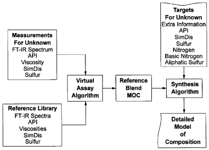
be inferred by extrapolating the gas oil compositions so as to be
consistent with other measurements such as elemental analysis
(C, H, S, N, 0, Ni and V), average molecular weight, Nuclear
Magnetic Resonance (NMR), infrared (IR), ultra-violet visible
(UV-visible) spectroscopy and separation techniques such as
short path distillation, high performance liquid chromatography
(HPLC), gas chromatography (GC) and solvent solubility.
= For wider boiling materials such as crude oils, the HDHA
analysis requires that the total material be distilled into naphtha,
kerosene, gas oil and resid fractions which are separately
analyzed via the protocols discussed above. The distillation can
be accomplished via methods such as ASTM D 2892 and D
2
CA 02740845 2011-04-14
WO 2009/051742 PCT/US2008/011796
1160. The data for the individual cuts is then combined into a
complete description of the wider boiling material.
[00041 HDHA compositions are currently measured on different process
streams. These detailed compositions are used in the development of SOL-based
refinery process models (see R. J. Quann and S. B. Jaffe (Ind. Eng. Chem. Res.
1992, 31, 2483-2497 and Quann, R.J.; Jaffe, S.B. Chemical Engineering
Science v51 n 10 pt A May 1996. p 1615-1635 , 1996), and serve as a reference
"template" of typical stream compositions. The HDHA method, while giving
detailed results, is also elaborate and expensive, and is not suited for on-
line
implementation. Therefore, when composition of a sample is required for use in
process control or optimization, synthesis techniques (step 2 of the current
invention) are typically used to adjust a fixed reference template selected
based
on prior experience to match measured property targets such as API and boiling
curve. However, systematic reference selection techniques do not exist and the
quality of the eventually estimated composition crucially depends upon the
reference. Estimating composition from properties can be difficult to
impossible
if poor judgment and criteria are used to select the reference. Availability
of a
whole sample, multivariate analytical techniques such as FTIR, supply a
crucial
piece of the composition puzzle that can be used to construct this critical
"reference" composition. Brown (US 6662116 B2) has described the use of
FTIR measurements and a "Virtual Assay" analysis methodology for estimating
for crude assay information. This analysis methodology can be used to estimate
HDHA data, but the resultant composition estimates may not adequately match
measured property values. The estimated compositions, however, are often
superior references for the synthesis of an accurate detailed composition.
SUMMARY OF THE INVENTION
[00051 Petroleum streams are complex mixtures of hydrocarbons containing
enormous numbers of distinct molecular species. These streams include any
hydrocarbon stream from processes that change petroleum's molecular
3
CA 02740845 2011-04-14
WO 2009/051742 PCT/US2008/011796
composition. The streams are so complex, and have so many distinct molecular
species that any molecular approximation of the composition is essentially a
model, that is, a model-of-composition (MoC)
[0006] The present invention provides a method for estimating the detailed
model-of-composition of an unknown material. The estimation method involves
two steps. The first step uses a multivariate analytical technique such as
spectroscopy, or a combination of a multivariate technique and sample property
analysis, (e.g. spectroscopy plus API, elemental data, viscosity and/or
boiling
curve), to construct an initial estimate of composition, e.g. a template
composition called "the reference". In the second step, this reference
composition is refined through an optimization algorithm to adjust the
template
composition to match a set of additional analytical data or properties called
"targets" (e.g. a distillation or simulated distillation curve) so as to
provide a
self-consistent model of composition for the unknown material. The specific
targets used in the second step may be sample type dependent, and they may
vary depending on the ultimate use of the composition data. The algorithm in
the second step minimally modifies the reference composition to preserve the
underlying molecular signature while attaining the target values. This latter
use
of a regression algorithm to adjust the reference composition so that it
matches
known property targets is referred to as "synthesis" or "tuning". The validity
of
this method is supported by examples where the initial reference is close to
the
measured composition and examples where the initial reference is far from the
measured composition.
[0007] Petroleum is a complex mixture containing thousands of distinct
hydrocarbon species including paraffins, cyclic paraffins, multi-ring
aromatics,
and various heteroatomic hydrocarbons (most commonly containing 0,S, and
N). Virgin petroleum crude oils contain molecules of a wide boiling point
range
from highly volatile C4 hydrocarbons to nonvolatile asphaltenes. Detailed
compositional analysis of petroleum is critical for determining the quality of
petroleum feedstreams, for determining the suitability of feedstreams for use
in
4
CA 02740845 2011-04-14
WO 2009/051742 PCT/US2008/011796
the manufacture of desired products, for developing process and refinery
models,
and for controlling and optimizing refining processes. Unfortunately, the
measurement of detailed compositional data has traditionally been both time
consuming and expensive, and such detailed composition data was seldom
available in timely fashion for decision making, control or optimization. The
current invention uses spectroscopy in combination with a few relatively
inexpensive and rapid property analyses to provide detailed estimates of
composition on a time frame suitable for decision making, control and
optimization.
[0008] Spectroscopy has been employed for compositional analysis of
petroleum, but such applications have been largely limited to analyses of
naphtha range materials where the number of molecular species is more limited,
or to the analysis of heavier feeds in terms of molecular lumps - groups of
molecules based on functional similarities. The use of spectroscopy to perform
step 1 of the current invention on crude oils has been previously described by
Brown (US 6662116 B2). Brown does not discuss the combination of the
spectroscopic analysis with synthesis (step 2 of the present invention) to
provide
an improved estimate of composition.
[0009] Currently, for petroleum process modeling, control and optimization,
a less detailed molecular lumping scheme may be employed so that the limited
composition may be estimated based on fewer, quicker and less expensive
measurements. Alternatively, a detailed composition may be estimated once,
and the composition is assumed to be sufficiently constant to allow the use of
this fixed detailed composition in modeling, control and optimization. Step 2
of
the present invention can be used to adjust this fixed detailed composition to
match property measurement data. The present invention provides maximum
benefit over current practices in instances where the stream being analyzed
varies widely over time, or where there is insufficient information to
establish a
suitable reference for Step 2.
CA 02740845 2011-04-14
WO 2009/051742 PCT/US2008/011796
BRIEF DESCRIPTION OF THE DRAWINGS
[0010] Figure 1 shows a schematic diagram of the procedure of the
invention described herein.
[0011] Figure 2 shows example target (WT) and reference (WD) boiling
point distributions.
[0012] Figure 3 shows a plot comparing the target (WT) and reference (WD)
cumulative distributions.
[0013] Figure 4 shows a how the factor, 0, used to adjust the reference
weights varies with boiling point.
[0014] Figure 5 shows a flowchart for the iterative model-of-composition
synthesis algorithm.
[0015] Figure 6 shows a parity plot comparing the MOC for Example 1,
Step 1 to the measured MOC.
[0016] Figure 7 compares the distillation calculated from the MOC of
Example 1, Step 1 to the measured distillation.
[0017] Figure 8 shows a parity plot comparing the MOC for Example 1,
Step 2 using bulk targets to the measured MOC.
[0018] Figure 9 compares specific gravity calculated from the MOCs for
Example I after Step 1, Step 2 using bulk targets, and Step 2 using
distributed
targets to the measured specific gravity.
[0019] Figure 10 compares sulfur calculated from the MOCs for Example 1
after Step 1, Step 2 using bulk targets, and Step 2 using distributed targets
to the
measured sulfur.
[0020] Figure 11 compares aliphatic sulfur calculated from the MOCs for
Example 1 after Step 1, Step 2 using bulk targets, and Step 2 using
distributed
targets to the measured aliphatic sulfur.
6
CA 02740845 2011-04-14
WO 2009/051742 PCT/US2008/011796
[00211 Figure 12 compares nitrogen calculated from the MOCs for Example
1 after Step 1, Step 2 using bulk targets, and Step 2 using distributed
targets to
the measured nitrogen.
[0022] Figure 13 shows a parity plot comparing the MOC for Example 2,
Step 1 to the measured MOC.
[0023] Figure 14 compares the distillation calculated from the MOC of
Example 2, Step 1, Step 2 using bulk properties and Step 2 using distributed
properties to the measured distillation.
[0024] Figure 15 compares the sulfur calculated from the MOC of Example
2, Step 1, Step 2 using bulk properties and Step 2 using distributed
properties to
the measured sulfur.
[0025] Figure 16 compares the aliphatic sulfur calculated from the MOC of
Example 2, Step 1, Step 2 using bulk properties and Step 2 using distributed
properties to the measured aliphatic sulfur.
[0026] Figure 17 compares the nitrogen calculated from the MOC of
Example 2, Step 1, Step 2 using bulk properties and Step 2 using distributed
properties to the measured nitrogen.
[0027] Figure 18 shows a parity plot comparing the MOC for Example 2,
Step 2 using bulk targets to the measured MOC.
[0028] Figure 19 shows a parity plot comparing the MOC for Example 2,
Step 2 using distributed targets to the measured MOC.
[0029] Figure 20 shows a parity plot comparing the MOC for Example 3,
Step 1 to the measured MOC.
[0030] _ Figure 21 shows a parity plot comparing the MOC for Example 3,
Step 2 to the measured MOC.
7
CA 02740845 2011-04-14
WO 2009/051742 PCT/US2008/011796
[0031] Figure 22 compares the distillation calculated from the MOC of
Example 3, Step 1 and Step 2 to the measured distillation.
[0032] Figure 23 shows a parity plot comparing the MOC for Example 4,
Step 1 to the measured MOC.
[0033] Figure 24 shows a parity plot comparing the MOC for Example 4,
Step 2 to the measured MOC.
[0034] Figure 25 compares the distillation calculated from the MOC of
Example 4, Step 1 and Step 2 to the measured distillation.
[0035] Figure 26 shows a parity plot comparing the MOC for Example 5,
Step 1 to the measured MOC.
[0036] Figure 27 shows a parity plot comparing the MOC for Example 5,
Step 2. to the measured MOC.
[0037] Figure 28 shows a parity plot comparing the MOC for Example 6,
Step 1 to the measured MOC.
[0038] Figure 29 shows a parity plot comparing the MOC for Example 6,
Step 2 to the measured MOC.
[0039] Figure 30 compares the distillation calculated from the MOC of
Example 6, Step 1 and Step 2 to the measured distillation.
[0040] Figure 31 shows a parity plot comparing the MOC for Example 7,
Step 1 to the measured MOC.
[0041] Figure 32 shows a parity plot comparing the MOC for Example 7,
Step 2 to the measured MOC.
[0042] Figure 33 compares the distillation calculated from the MOC of
Example 7, Step 1 and Step 2 to the measured distillation.
[0043] Figure 34 shows sample homologous series core structures.
[0044] Figure 35 shows saturate cores.
8
CA 02740845 2011-04-14
WO 2009/051742 PCT/US2008/011796
[0045] Figure 36 shows 1-ring aromatic cores.
[0046] Figure 37 shows 2-ring aromatic cores.
[0047] Figure 38 shows 3-ring aromatic cores.
[0048] Figure 39 shows 4-ring aromatic cores.
[0049] Figure 40 shows sulfide cores.
[0050] Figure 41 shows polar cores.
[0051] Figure 42 shows olefin and thiophene cores.
[0052] Figure 43 shows an example of an analytical scheme for measuring
the MOC of a vacuum gas oil.
DETAILED DESCRIPTION OF THE PREFERRED EMBODIMENTS
[0053] Petroleum mixtures are made up of an exceedingly large number of
individual molecular components. These streams are so complex, and have so
many distinct molecular species that any molecular approximation of the
composition is essentially a model, i.e. a model-of-composition. Such a model-
of-composition is used to simulate the physical and chemical transformations
that occur in refinery processes, and to estimate the properties of the
various
petroleum feed and product streams. Analytical methods for approximating the
detailed compositional profile of petroleum mixtures as a large, but finite,
number of components already exist. For instance, High Detailed Hydrocarbon
Analysis (HDHA) is a protocol used in ExxonMobil to represent complex
petroleum mixtures as an internally consistent set of components. The HDHA
protocol for a petroleum mixture yields a model-of-composition. Process and
product property models (see for example Ghosh, P., Hickey, K.J., Jaffe, S.B.,
"Development of a Detailed Gasoline Composition-Based Octane Model", Ind.
Eng. Chem. Res. 2006, 45, 227-345.and Ghosh, P., Jaffe, S.B., "Detailed
Composition-Based Model for Predicting the Cetane Number of Diesel Fuels",
Ind. Eng. Chem. Res. 2006, 45, 346-351.) built on this model of composition
are
9
CA 02740845 2011-04-14
WO 2009/051742 PCT/US2008/011796
used in a large number of engineering and business applications such as plant
optimization, raw materials acquisition and process troubleshooting. Several
of
these stream properties are computed from correlations in which molecular-lump
property densities take simple blending rules (e.g. linear) with respect to
their
wt% abundances in a stream's model-of-composition (see Section on Property
Correlations below). However, development of detailed crude oil and plant
stream analytical data to support these activities can be time consuming and
expensive. The ability to estimate such compositions quickly and cheaply from
limited amounts of measurements on any given sample would enhance the
applicability and utility of these applications, reduce associated costs, and
reduce
R&D cycle times significantly. It would also facilitate development of on-line
composition.. inference protocols that could be used to improve applications
such
as Real Time Optimization (RTO), and may have applicability to on-line
blending.
[0054] The current invention provides a more rapid and less expensive
means of estimating a detailed composition for a crude oil or petroleum
mixture
in two steps. In the first step, a "reference" or "template" composition is
estimated from multivariate analytical data alone, or in combination with a
small
set of measured properties using the method of Brown. In the second step, this
reference composition is refined to match a set of measured properties using
an
optimization algorithm referred to as "synthesis" or "tuning". We have found
that this "reference" (or "template") composition (defined in terms of a
specified
model of composition) of an unknown petroleum crude or fraction, can be
obtained through the use of (1) multivariate analytical techniques such as
FTIR
alone, or in combination with a small set of appropriately chosen property
measurements of the sample whose composition is sought, (2) a library
(database) of similar samples that have measured multivariate analytical data
(FTIR), measured HDHA and measured properties and (3) an optimization
algorithm as described by Brown which constructs the reference composition for
the sample as a blend of similar samples in the library so that the
multivariate
CA 02740845 2011-04-14
WO 2009/051742 PCT/US2008/011796
(FTIR) and property data for the blend is consistent with the multivariate
(FTIR)
data and property made on that sample. The synthesis algorithm is then applied
to adjust the reference composition to meet known properties of the unknown
sample. The different steps of this procedure are illustrated schematically in
Figure 1.
[0055] The property measurements used in steps 1 and 2 may include but
are not limited to API gravity, viscosity, distillation or simulated (GC)
distillation (SimDis, for instance ASTM D 2887), sulfur content, nitrogen
content, aliphatic sulfur content, and basic nitrogen content. The properties
used
in step 1 may be the same or different from those used in step 2.
.Step 1: Estimating the "Reference" Composition
[0056] Brown (US 6,662,116 B2 and US 2006/0047444 Al) described how
an unknown crude oil can be analyzed as a blend on known crude oils based on
fitting the FT-IR spectrum of the unknown alone, or in combination with
inspections such as API gravity and viscosity as a linear combination of
spectra
and inspections of reference crudes. This method is used to estimate assay
data
for the unknown crude based on the calculated blend and the assay data of the
reference crudes. Similarly, this method can be used to estimate a reference
HDHA for the unknown crude based on the calculated blend and the measured
HDHA of the reference crudes. The method can also be employed for analysis
of petroleum feed and product streams. In Step 2, this reference HDHA can then
be tuned to measured assay properties to yield an accurate estimate of the
detailed composition of the unknown crude/stream.
[0057] If the FT-IR spectrum is used alone, then the analysis involves the
minimization of the difference between the FT-IR spectrum of the unknown and
that calculated as the linear combination of the FT-IR spectra of the blend of
the
reference crudes.
min((zu - xuf(Cu - xõ)) [1a]
11
CA 02740845 2011-04-14
WO 2009/051742 PCT/US2008/011796
xõ=Xcu [lb]
[0058] xu is a column vector containing the FT-IR for the unknown crude,
and X is the matrix of FT-IR spectra of the reference crudes. The FT-IR
spectra
are measured on a constant volume of crude oil, so they are blended on a
volumetric basis. Both x,, and X are orthogonalized to corrections (baseline
polynomials, water vapor spectra, and liquid water spectra) as described in US
6,662,116 B2.
[0059] To ensure that the composition calculated is non-negative, the
minimization is conveniently done using a non-negative least squares. The
analysis provides coefficients for a linear combination of the reference
crudes
that most closely matches (in a least squares sense) the spectrum of the
unknown
crude.
[0060] US 6,662116 and US 2006/0047444 Al also describes an analysis
of crude oil based on FT-IR data augmented with API Gravity and kinematic
viscosity. The algorithm attempts to minimize the difference between the data
for the unknown crude and that calculated for a blend of reference crudes
using
[2]
xu xu xu xu
T
min WAPj% (AP/) - WAPj2 (API) WAPj2u(API) - WAPIAu(APl) [2a]
WV1. Au(Visc) WVisc2u(Visc) WVisc)u(Visc) WViscAu(Visc)
zõ = Xcu., 2u(API) = A(API)cu , and )t (visc) = A(visc)cu [2b]
xu is a column vector containing the FT-IR for the unknown crude, and X is the
matrix of FT-IR spectra of the reference crudes. The FT-IR spectra are
measured on a constant volume of crude oil, so they are blended on a
volumetric
basis. Both xu and X are orthogonalized to corrections (baseline polynomials,
water vapor spectra, and liquid water spectra). xu is augmented by adding two
12
CA 02740845 2011-04-14
WO 2009/051742 PCT/US2008/011796
additional elements to the bottom of the column, wp A,,(AP1) , and
wvisc/lu(visc) .
A,,(api) and llu(visc) are the volumetrically blend-able versions of the API
gravity
(i.e. specific gravity) and viscosity for the unknown, and A(API) and A(vlsc)
are the
corresponding volumetrically blend-able inspections for the reference crudes.
wAp1 and w,,;sc are the weighting factors for the two inspections. The 2u and
Au values are the estimates of the spectrum and inspections based on the
calculated linear combination with coefficients cu. The linear combination is
preferably calculated using a nonnegative least squares algorithm. The
weights,
w, in [2] have the form [3].
. 2.77=a e
w=
R
[3]
R is the reproducibility of the inspection data calculated at the level for
the
unknown being analyzed. E is the average per point variance of the corrected
reference spectra in X, and is set to 0.005 for crude or intermediate stream
spectra collected in a 0.2-0.25 mm cell. a is an adjustable parameter. a is
chosen by an optimization procedure described below.
[0061] For analysis of kerosene and gas-oil petroleum streams using FT-IR
augmented with Simulated Distillation (SimDis) data, algorithm of US 6,662116
was modified to allow for use of inspections including ones where there is
more
than one value per sample. When using three inspections, the current invention
minimizes
13
CA 02740845 2011-04-14
WO 2009/051742 PCT/US2008/011796
T,-
X, Xu Xu
Xu
WAPI2u(API) WAPIJIu(API) WAPlZu(API) WAPI2u(API)
WE30011v(E300) WE3001lu(F.300) WE3002u(E300) 1'VE30011u(E300)
WE400Au(E400) WE4001lu(E400) WE400Au(E400) WE4002u(E400)
WE500Au(E500) WE5001lu(E500) WE50OAu(E500) WE500Aw(E500)
min WE600Au(E600) - WE6001lu(E600) WE6002U(E600) - WE600a'u(E600)
WE7002u(E700) WE700Au(E700) WE7002u(E700) WE7002u(E700)
WE800a'u(E800) WE8002u(E800) WE8002u(E800) WE800a'u(E800)
WE9002u(E900) WE9002u(E900) WE9002u(E900) WE900.u(E900)
WE1000Au(E1000) WEIooo2 (EI000) WEIOOOAu(E1000) WEI000IU(EI000)
WSuI/Iu(Sul) WSul2u(Sul) wsul)u(Sul) WSulAu(sul)
[3a]
Xu = XCu , 2u(API) = A(API )Cu , /Zu(E300) = A(E300)Cu , ... 2u(Sul) =
A(sul)cu [3b]
[0062] The Au(E3oo) represents the volumetrically blend-able SimDis data.
SimDis data is typically reported as temperatures for fixed weight percent
off,
and is thus cannot be used not directly. The SimDis data is converted to a
volumetrically blend-able form in two steps: (1) the SimDis curve is
interpolated
using a cubic interpolation and the curve is evaluated at points spanning the
temperature range of interest, for instance at 300, 400, 500, 600, 700, 800,
900 F
points. and 1000 F; if the SimDis range does not span these temperatures, the
data is augmented with zeros below or 100% above to ensure proper behavior of
the cubic interpolation at the endpoints. (2) the weight percent of sample
evaporated at each temperature is multiplied by the sample specific gravity to
give a volumetrically blend-able value. A(E300) is the corresponding data for
the reference samples. ..% (E3oo) is the estimate of 2u(E3oo) based on the
linear blend
with coefficients cu. .% (sul) is volumetrically blendable sulfur data for the
unknown, generated as the weight percentage sulfur times the sample specific
gravity, A(Sul) is the corresponding data for the reference samples, and
2u(sul) is
the estimate of 2u(sul) based on the linear blend.
[0063] For the weighting of the SimDis data in [3 a], the adjustable
parameter, a, may be set to the same value for all SimDis points.
Alternatively,
14
CA 02740845 2011-04-14
WO 2009/051742 PCT/US2008/011796
since the SimDis data is least accurate near the initial boiling point and
final
boiling, point, the weights of temperatures that fall below some minimum
cutoff
(e.g. 5% off) or above some maximum cutoff (e.g. 95% off) for the unknown
being analyzed may be set to zero so as to use only the more accurate SimDis
data. The value of a is determined by an optimization procedure designed to
maximize the accuracy of the reference HDHA. One such optimization
procedure is described in Appendix D.
[00641 Once the coefficients c, for the blend are calculated, the HDHA for
the unknown is estimated as the corresponding blend of the HDHAs of the
reference samples. Note that if the analysis is done using a multivariate
analytical technique such as FT-IR, the coefficients c,, will represent volume
fractions of the references in the blend. Since the HDHA data will typically
be
expressed on a weight or weight percentage basis, a conversion from volume to
weight basis is required. If h is a vector of HDHA data for a reference
sample,
then h can be converted from weight fraction (or percentage) to volume
fraction
(or percentage) by dividing each element of h by the specific gravity of the
corresponding molecule, and renormalizing the resulting vector to sum to unity
(or 100%) to produce a volumetric representation of the HDHA. The volumetric
vectors for the references are combined in the proportions indicated by the
coefficients c,, to produce a volumetric HDHA vector for the unknown. Each
element of the vector is multiplied by the specific gravity of the
corresponding
molecule, and the vector is renormalized.to sum to unity (or 100%) to produce
the weight :action (or percentage) based HDHA estimate for the unknown.
Step 2: Synthesis: Reconciling Analytical Measurements to the Model-of-
Composition
[00651 The second step of this invention is to reconcile analytical
measurements to the model-of-composition. In particular, the model-of-
composition must reproduce all measurements in the analytical protocol as
closely as possible, and at the same time satisfy a set of property balances,
e.g.
CA 02740845 2011-04-14
WO 2009/051742 PCT/US2008/011796
mass and elemental composition. Often, these property balances are expressed
N
as a system of linear equations, e.g. bj = Zajiwi. Here, the measured value of
the
i=1
property in thej-th balance is bj. The density of propertyj in molecular lump
i is
aji.. The wt% abundance of molecular lump i in the MoC is wi... The property
densities aji.. are either computed directly from each lump's elemental
composition, or are correlated to measurements conducted on samples of known
composition.
[0066] One embodiment of this reconciliation procedure is to treat it as a
constrained optimization problem: we optimize the model-of-composition's
fidelity to the test results of the analytical protocol subject to the
property
balance constraints. Another embodiment of the reconciliation procedure is
successive substitution, an iterative procedure in which the model-of-
composition is adjusted to match the results of the analytical protocol in a
prescribed sequence until changes in the model-of-composition between
iterations fall below a prescribed tolerance.
a) Reconciliation by Constrained Optimization
[0067] In the constrained optimization embodiment, we start with a model-
of-composition whose reference molecular lump weight percents {w1 *} exactly
the results from Step 1. Next, we seek a new set of weight percents {wi } that
are
minimally different from those of the reference, yet satisfy the property
balances
described above. To find these weight percents, we minimize the Lagrangian L
(see Denn, M. M. "Optimization by Variational Methods", Chapter 1,
McGraw-Hill, NYC, 1969.), defined by:
N NP N
L = Z Wi * ln(wi 1 wi *) + Z Aj bj - N aji w!
i=1 j=1 i=1
(4)
[0068] The first term in Equation (4) is the Shannon information entropy
content of the model-of-composition's weight percents {w, } relative to that
of the
16
CA 02740845 2011-04-14
WO 2009/051742 PCT/US2008/011796
reference weight percents {wi *} (see e.g. Cover, T. M. and J. A. Thomas,
"Elements of Information Theory", p. 18. J. Wiley & Sons, 1991) 'i is the
Lagrangian multiplier of thej-th property balance constraint. NP is the total
number of property balances considered in reconciliation. N is the number of
molecular lumps in the model of composition. The Lagrangian L is minimized
when the following stationary conditions are satisfied:
SL aL
0 for j =1,...,NP
Srv 0 ' aAj.
(5)
[0069] From aL / aa.; = 0 we recover the linear property balance equations
N
bi _ aii wi . We evaluate the functional derivative 8L / & using calculus of
variations (see e.g. Davis, H. T., "Statistical Mechanics of Phases,
Interphases
and Thin Films", Chapter 12, VCH Publishers, 1996.). For the Lagrangian in
Equation (6), the stationary solution is
NP
w1 =w1 *exp -1+aA for i=1,...,N
J=1
(6)
[0070] Next, we substitute the stationary solution (7) into the property
balance equations and eliminate the unknown weight percents {wi 1:
N NP
I ajjwj *exp(-1+>2kaki)=bj for j =1,...,NP
i=1 k=1
(7)
[0071] We solve the nonlinear algebraic equations (7) on a digital computer
for the Lagrangian multipliers {2k } using Newton's method. Once we have
solved the equation system (7) for these Lagrangian multipliers, we substitute
them into the stationary solution (6) and obtain the weight percents of the
reconciled model-of-composition {W, } .
17
CA 02740845 2011-04-14
WO 2009/051742 PCT/US2008/011796
[0072] In the above embodiment of the reconciliation algorithm, linear
property balance equations make the Lagrangian L (see Eqn. (4)) convex; i.e.
one and only set of weight percents {w; } both locally and globally minimize L
(see Ref. " (see e.g. Cover, T. M. and J. A. Thomas, "Elements of Information
Theory", p. 14. J. Wiley & Sons, 1991). Thus, linear property constraint
equations are preferred in the above embodiment of the reconciliation
algorithm.
However, nonlinear property balances constraints may be used. In this
embodiment, the Lagrangian L reads
N NP
L = w, *ln(w;/w;*)+ZA,j (bj -Aj ({w;})) (7a)
where the property function Aj({w; }) is any twice-differentiable function of
the
molecular lump weight percents {w; } . Examples include: nonlinear algebraic
equations, or the output of any algorithm that takes the molecular lump weight
percents {w; } as inputs. In the latter example, the first and second
derivatives of
the property function A j ({w; }) with respect to molecular lump weights wjcan
be
approximated by finite-differences (see e.g. Numerical Analysis, Burden, R.L.,
J. D. Faires, A. C. Reynolds (ed.), 2nd Ed., Prindle, Weber & Schmidt
(publishers), NYC, pp. 124-132).
As in the linear constraint embodiment, we recover the property
balance equations bj = Aj({w; }) from the stationary solution condition
aL / aAj = 0 when imposed on the Lagrangian L shown in Eqn. (7a). Similarly,
the stationary solution condition &L / &w = 0 reads
NP aA
w; = w; * exp I+ N ' (7b)
J=1
where the unknown weight percents {w; } cannot be readily eliminated as
unknowns, as in the linear constraint embodiment detailed above. Instead, the
equation system (7b) and the property balance equations bj = Aj({w; }) must be
18
CA 02740845 2011-04-14
WO 2009/051742 PCT/US2008/011796
solved iteratively for both the unknown weight percents {w; 1, and the
Lagrangian multipliers {Ak } . Newton's method can comprise this iterative
scheme if the property balance functions Aj({w; }) are twice-differentiable
with
respect to the weight percents wj, (see above). However, if the property
functions Aj({w; }) are nonlinear, the Lagrangian L shown in Eqn. (7a) may or
may not be convex, and multiple solutions to the unknown weight percents
{w; 1, and the Lagrangian multipliers {/zk } are possible.
b) Reconciliation by Successive Substitution
[0073] As in the constrained optimization reconciliation method described
above, this embodiment of the reconciliation procedure also starts with model-
of-composition whose reference molecular lump weight percents {w; *} exactly
the results from Step 1. Adjustments to the weight percents {w; *} are done in
sequence, i.e. the reconciled weight percents {w; } computed from the j-the
property balance become the reference weight percents {w; *} of the j+1-th
property balance. Below we describe weight percent adjustment formulae for a
scalar and distributed property targets, and the successive substitution
reconciliation algorithm.
a) Scalar Property Targets
[0074] Scalar properties take a single number for the entire sample.
Simple ratio properties
[0075] A simple ratio property is linear in weight percents, its property
density_aj, is nonzero for selected molecules, and equals zero for others.
Examples of simple ratio properties include elemental composition. For simple
ratio properties, we combine the property balance with a total mass balance to
obtain:
19
CA 02740845 2011-04-14
WO 2009/051742 PCT/US2008/011796
w; = W, * N b' for ai; > 0
E aikWk
k=1
(8)
[0076] Once we have adjusted (ratioed) the weight percents of molecules
that possess the simple ratio propertyj, we adjust the weights of the
molecules
that do not possess this property:
100-> Wk
a1k>0
k for aj;=0
w,=w; w
a/k =0
(9)
Averaged properties
[0077] Averaged properties are scalar properties whose property densities
ai; # 0 for all molecular lumps i =1, ... , N. Examples of such averaged
properties include API gravity, hydrogen content, octane number, and pour
point. For averaged properties, the ratio method summarized in Equations 8 and
9 will not work. Instead, we have developed a factor 0 that is a continuous
function of the averaged propertyj whose target value equals bj. This factor
adjusts upward the weights of molecules whose property density ai; is less
than
that of the target bj., and it adjusts downward the weights of molecules whose
property density ai; is greater than the target value bj. The net result is to
shift
the distribution of weights {w1 } toward a distribution that satisfies the
property
N
constraint equation a;1 w; = bi
~=1
[0078] The continuous factor 0 takes a cubic polynomial in the property
value b:
O(b) = Al b 3 +A 2 b 2 + A3b + A4
(10)
CA 02740845 2011-04-14
WO 2009/051742 PCT/US2008/011796
[00791 We determine the four constants A, through A4 with the following
constraints:
N
Conservation of total weight: 100 = w; q5 (1l a)
N
Averaged property constraint: b j = a Ji w; q$ (11 b)
[0080] Smoothness at extreme values of the propertyj:
0 = aO at b = bmin,J (11c)
0 = ao at b = bma J (11 d)
[0081] After we impose the constraints (11 a-d) upon the factor 0 defined in
Equation 10, the factors and adjusted weights {w, } are computed as follows:
0=1+rAb;
(12)
N
bJ -Ewi *aj;
y _ N i=1
aJ;wi *Ab;
;=1
(13)
N
3 2
aJiwi* 3b +b apwi*
3 ;=1 .in, j ,J) 2 _
a 3 - N - a J; N
Ew 2 Ew
Abi - i=1 i=1 (14)
aii W,
+ 3(b min J + bm J) a Ji - `='N
Ew;
;=1
w; =w;*(1+rAb;)fori=1,...,N
(15)
21
CA 02740845 2011-04-14
WO 2009/051742 PCT/US2008/011796
[0082] We avoid the occurrence of 0<0 by restricting the property target
range (b",;õ j , b,,,aj). If the actual target bi is outside this range, we
approach this
target in multiple steps.
[0083] In the case of multiple average property targets, we may calculate
separate weight factors q, for each target propertyj. However, we have
achieved
much greater effectiveness by using a single factor that includes the
dependence
of all averaged property targets. The factor adds all cubic polynomials
together
in Equation 10, with three additional parameters for each target. Constraints
in
Equation 11 are also used for each property. Final factors and weight
adjustments are similar in form to Equations 12-15.
Distributed Property Targets
[0084] In general, a distributed property target occurs when the property to
be matched varies with some independent variable. The distribution of weight
distilled with boiling point temperature, i.e. the distillation curve, is the
most
frequently encountered distributed target. In the successive substitution
method,
we design a factor 0 that effectively "redistills" the reference weight
distribution
{w; *} during each iteration of the reconciliation algorithm we describe
below.
[00851 Let W(BP) represent the cumulative weight percent distilled off at
boiling point BP. The measured target distribution is WT, and Wo is calculated
from the reference weight distribution {w; *} of the molecular lumps. Both of
these cumulative weight distributions are monotonically increasing functions
of
the boiling point BP (see Figure 2). In practice, the cumulative weight
distribution W,. is measured at discrete boiling points. Also, we calculate
the
distribution Wo at the boiling points of each molecular lump. However, we may
interpolate between these discrete boiling points using smooth functions that
preserve the monotonically increasing nature of a cumulative weight
distribution. After this interpolation, we determine the target distribution
W,. as a
22
CA 02740845 2011-04-14
WO 2009/051742 PCT/US2008/011796
function of the calculated distribution WD at the same distillation boiling
points
(see Figure 3). Finally, we calculate the factor 0 - dWT / dWo as a function
of
boiling point (see Figure 4). We use the factor 0 to adjust the reference
weights
as follows:
100w1 * O(BF)
W; = N for i=l,...,N (13)
2: w; *q$(BP;)
J=1
where BPi is the boiling point of molecular lump i.
c) The Successive Substitution Reconciliation Algorithm
[0086] In Figure 5, we show the typical embodiment of the successive
substitution reconciliation where a reference model-of-composition is adjusted
to
match one distributed target (boiling point), and more than one scalar
property
targets. In general, adjusting weight percents to match each target in
sequence
disrupts the previous match so that the weight percent adjustments are
relaxed,
or dampened, to ensure convergence of the successive substitution algorithm.
d) Targets based on multivariate analytical measurement
[0087] The targets used in reconciliation may include ones estimated based
on the multivariate analytical data used Step 1 of the invention. These
targets
may be calculated based on the reference composition determined from Step 1.
Alternatively, these targets may be estimated via regression models developed
for this purpose. Such regression models, can be developed using standard
chemometric techniques such as Multilinear Regression (MLR), Principal
Components Regression (PCR), or Partial Least Squares (PLS) or via the method
of Brown (US 5121337, June 9, 1992). The multivariate analytical data for the
references in the library database for Step 1 are regressed against measured
target data to form a predictive model. This model may then be applied to the
multivariate data for the unknown being analyzed to estimate a target to use
in
Step 2. For example, a regression model can be built to relate FT-IR spectra
of
the references to aromatic carbon content measured by NMR. Said model is
23
CA 02740845 2011-04-14
WO 2009/051742 PCT/US2008/011796
used to estimate an aromatic carbon content target for the sample being
analyzed.
Examples 1 & 2
[0088] The current invention can be used to estimate a composition for a
crude oil, or distillation cuts thereof. In Step 1, the methodology of US
6,662116 and US 2006/0047444 Alis used to estimate a blend of reference
crudes for which models of composition have been measured. The blend of
these models of composition serves as a reference for subsequent synthesis in
Step 2. If the crude oil being analyzed is one for which crude assay data was
either measured, or estimated using the methods of US 6,662116 or US
2006/0047444 Al, then properties estimated from the model of composition
match those of the assay. In this case, the targets used in the Step 2
synthesis
will typically be distributed targets (property values as a function of
boiling
point) rather than bulk targets (properties of the whole sample). Examples 1
and
2 compare models of composition built using bulk and distributed targets.
[0089] The validity of the technique was demonstrated as follows. A library
of 73 crudes was collected, every member of which had, (i) a measured HDHA
composition, (ii) a measured assay, (iii) a FTIR spectrum and (iv) other bulk
properties (including API gravity and viscosity). A series of test runs (known
as
cross-validation runs) were conducted by selectively removing one crude at a
time from the library and treating it as a sample of unknown composition, in
order to estimate its composition from the remaining 72 crudes using the
procedure outlined above. Each test run consisted of three steps. First, a
blend of
the 72 crudes was constructed that best matched the FTIR spectrum, API and
viscosity of the sample removed using the methodology of US 6,662116 and US
2006/0047444 Al. Next, the HDHA based compositions of the 72 crudes were
blended in proportion of the blend suggested in the previous step to obtain
the
"reference" composition. Finally, the synthesis algorithm was applied on the
reference composition to match additional measured either bulk or distributed
24
CA 02740845 2011-04-14
WO 2009/051742 PCT/US2008/011796
targets of the removed sample, such as gravity (API or specific), the boiling
curve, nitrogen, basic nitrogen, sulfur and aliphatic sulfur. The estimated
composition was then compared to the actual measured composition available
from the removed sample's HDHA.
Example 1
[0090] An MSO Edmonton crude oil was analyzed using the method of this
invention relative to the remaining 72 crudes in the library. In the first
step, the
spectrum, API gravity and viscosity of the crude oil are used as inputs, and
the
method of US 6,662116 is used to calculate a blended reference. The blend
recipe is shown in Table 1.
Table 1
Component % Component %
WEST TEXAS 17.89 WEST TEXAS 4.63
INTERMEDIATE SOUR
MESA 30 13.59 ZAFIRO 2.4
ELK BASIN HEAVY 12.71 URALS 2.21
MARGHAM CONDENSATE 10.36 OSO 2.19
CONDENSATE
QATAR MARINE 8.05 HAWKINS MIX 1.88
SMILEY COLEVILLE 7.36 SYNCRUDE 1.86
OSEBERG BLEND 6.39 FORCADOS 1.55
MIDALE 6.2 VASCONIA BLEND 0.74
[0091] Figure 6 compares the weights for the model of composition
calculated from this blended reference (y-axis, MOC predicted after step 1) to
those measured for the MSO Edmonton crude (x-axis, MOC actual wt%).
Brown (US2006/0047444 Al) defined a Fit Quality Ratio (FQR) as a measure of
how well the spectrum and inspections of the unknown (MSO Edmonton) are
matched by the calculated blend, a value of less than 1 being very good fits,
between 1 and 1.5 acceptable and larger values indicative of poorer fits. An
FQR of 1.02 was obtained in this example indicating the blend is a reasonably
good match to the sample being analyzed. In Figure 6, the diagonal parity line
represents complete agreement between the MOC estimated by step 1 of the
current invention and the measured MOC. The fact that most MOC components
CA 02740845 2011-04-14
WO 2009/051742 PCT/US2008/011796
fall close to the parity line demonstrates the ability of the FTIR based
blending
algorithm to capture the significant molecular trends of the actual
composition in
the reference. The correlation coefficient between the estimated and measured
MOCs is 0.9467. Despite this good agreement, properties calculated from the
blended reference MOS are not in complete agreement with those measured.
For example, the 30.45 API gravity calculated from the blended reference MOC
is higher than the 28.98 measured value (Table 2). Similarly, the estimated
distillation curve (Figure 7 dashed line) does not exactly match the measured
distillation (Figure 7 open circles).
[00921 Figure 8 compares the weights for the model of composition after
step 2 synthesis to bulk properties (y-axis) to those measured for the MSO
Edmonton crude (x-axis). The step 2 synthesis provides only marginal
improvment in the correlation coefficient (0.9630 after synthesis), but the
MOC
now more closely matches the measured property targets. From Table 2, the
API and Sulfur agree exactly with the measured targets. From Figure 7, the
estimated distillation (solid curve) now agrees more closely with the measured
data (open circles). Figures 9-12 compare the property values for the model of
composition after step 1 (dashed lines), step 2 synthesis to bulk properties
(dash-
dot lines), step 2 synthesis to distributed properties (solid lines) to the
measured
property data (open circles. Since the blended reference is a very good
approximation of the composition, the distributed properties only move
slightly
during synthesis as shown in Figures 9-12. For synthesis to bulk properties,
there are minor differences between the estimate property distributions
generated
using this invention (dash-dot lines) and those measured (open circles), even
for
those properties that are used as targets. However, for synthesis to
distributed
targets (solid lines), the estimated property distribution for the target
properties
agree with those the measured data. The result demonstrates how the synthesis
allows for a match to all these targets while retaining the correct structure
of the
compositional patterns.
26
CA 02740845 2011-04-14
WO 2009/051742 PCT/US2008/011796
Table 2
Actual Blended Tuned to Bulk Tuned to Dist
Reference Targets Targets
API 28.98 30.45 28.98 28.54
SAT wt% 64.4 65.2 62.6 61.5
n-PAR wt% 12.05 11.23 10.8 10.16
i-PAR wt% 12.37 15.93 14.3 13.6
1-ring 19.04 20.2 18.75 18.61
2-ring 12.55 12.25 12.32 12.66
3-ring 5.74 4.41 4.89 5
4-ring 2.11 1.07 1.33 1.32
5-ring 0.5 0.12 0.16 0.16
6-ring 0.03 0.03 0.03 0.03
S wt% 1.05 1.01 1.05 1.05
aliph S wt% 0.33 0.32 0.33 0.33
tot N ppm 615.32 536.36 615.62 607.7
basic N ppm 187.14 187.35 187.94 185.43
H2 wt% 12.81 12.9 12.75 12.69
POLAR wt% 0.53 0.53 0.56 0.53
ARO+SUL wt% 35.07 34.23 36.88 37.93
ARC 1 13.47 13.44 14.02 14.51
ARC2 10.17 10.07 10.78 11.44
ARC3 5.76 5.37 6.04 6.1
ARC4 2.96 2.52 3.03 2.91
RI 70 1.4703 1.4668 1.4716 1.473
%CA 16.11 15.79 16.94 17.56
pour pt C 24.1 20.5 21.7 20.7
cloud pt C 31.8 30.8 30.4 29.7
freeze pt C 31.8 30.8 30.4 29.7
TAN mg/g 0.2 0.2 0.2 0.2
Example 2
[00931 A Brookland crude was analyzed relative to the 72 other reference
crudes in the library. The blend calculated from Step 1 is shown in Table 3.
Note in this case, the FQR statistic is 2.43 indicating that, because of the
small
library size, the blend is not a good match to the crude being analyzed. As
seen
in Figure 11, there is poorer agreement between the MOC weights predicted
from the bli,-nded reference.(y-axis) and those measured for the Brookland
crude
(x-axis). The correlation coefficient is 0.9467. From Table 4, and Figures 14-
17
compare the properties calculated from the blended reference MOC (Table 4,
column 3 and Figures 14-17 dashed lines) to those measured for Brookland
crudes (column 2 and open circles). The model of composition for the blended
reference (curves) differs significantly from the actual measured crude MOC,
27
CA 02740845 2011-04-14
WO 2009/051742 PCT/US2008/011796
particularly in terms of the aromatic and sulfide components.
Table 3
Component %
N"KOSSA 40.99
MARGHAM 34.22
CONDENSATE
TENGIZ 14.82
TAPIS 8.96
COOPER BASIN 1.01
[0094] Figures 18-19y show the weights for MOC results of step 2
synthesis to bulk and distributed properties respectively. In both cases,
targets
included gravity, boiling curve, sulfur, aliphatic sulfur, nitrogen and basic
nitrogen. The synthesized models of composition are much closer matches to
the measured model of composition, particularly with respect to the aromatics
and sulfides. Figures 14-17 show property predictions for the various models
of
composition (dashed curves for Step 1 MOC, dash-dot curve for MOC after Step
2 synthesis with bulk property targets, and solid curve for MOC after Step 2
synthesis with distributed targets) compared to those based on the measured
model of composition (open circles). Table 4 summarizes some key properties.
[0095] This example illustrates that while the reference selection procedure
may sometimes suffer from lack of adequate references in the FTIR-HDHA
library, it can, with the synthesis procedure, still estimate the composition
to a
reasonable degree of accuracy. Given the cost of generating the MOC reference
data, this extended applicability increases the value of this two step
procedure
relative to that of Step 1 (US 6,662,116) alone.
Table 4
Actual Blended Tuned to Bulk Tuned to Dist
Reference Targets Targets
API 39.99 37.7 39.98 38.93
SAT wt% 88.7 82.1 88.6 86.6
n-PAR wt% 22.16 20.97 24.35 22.45
i-PAR wt% 28.46 20.6 23.89 21.87
Naphthenes
1-ring 23.06 23.79 24.49 24.94
2-ring 11.04 11.65 11.12 11.94
28
CA 02740845 2011-04-14
WO 2009/051742 PCT/US2008/011796
3-ring 3.36 4.11 3.84 4.26
4-ring 0.41 0.76 0.72 0.87
5-ring 0.12 0.21 0.18 0.24
6-ring 0.060 0.030 0.020 0.020
S wt% 0.030 0.170 0.030 0.030
aliph S wt% 0.010 0.050 0.010 0.010
tot N ppm 53.330 144.070 53.410 53.770
basic N ppm 18.840 36.700 20.200 18.910
H2 wt% 14.140 13.740 14.170 14.040
POLAR wt% 0.060 0.120 0.060 0.070
ARO+SUL 11.27 17.77 11.33 13.34
wt%
ARC 1 6.13 9.36 7.18 8.06
ARC2 3.32 5.08 2.72 3.47
ARC3 1.31 2.15 1.09 1.35
ARC4 0.4 0.73 0.27 0.36
RI 00 1.4384 1.4448 1.4377 1.4405
%CA 5.45 9.16 4.95 5.99
pour pt C 35.3 16.4 24.5 21.6
cloud pt C 57.3 38.8 43.5 41.6
freeze pt C 57.3 38.8 43.5 41.6
TAN mg/g 0 0.1 0 0
Examples 3-7
[00961 For examples 3-7, a library of 705 process stream samples was used.
These samples are kerosene and gasoil range materials which are feeds and
products of various refinery processes. For each of the 705 samples, an FT-IR
spectrum was collected covering the 5000-400 cm' range using a 0.25 mm fixed
path flow cell with CaF2 windows. Samples were maintained at 65 C. during
spectral data collection. For each sample in the library, HDHA was measured,
as were various bulk properties including but not limited to API gravity,
SimDis,
sulfur, aliphatic sulfur, nitrogen, and basic nitrogen. The HDHA of the
reference
samples were tuned to the measured bulk properties.
[00971 A cross-validation analysis was conducted in which each of the 705
samples were taken out of the library and treated as an unknown, being
analyzed
relative to the remaining 704 samples. The analyses were conducted in two
modes: (1) in the IR-Only mode, the FT-IR spectrum of the unknown was fit as a
linear combination of the remaining 704 spectra over the spectral ranges from
4998.6-3139.5 cm', 2760.6-2400.9 cm', 2200.4-1636.3 cm' and 1283.4-925.7
29
CA 02740845 2011-04-14
WO 2009/051742 PCT/US2008/011796
cm'. Spectral data in the 3139.5-2760.6 cm' and 1636.3-1283.4 cm' ranges
was not used since the absorbances in these ranges exceeded the linear
response
range of the FT-IR detector. Data in the 2400.9-2200.4 cm' range was not used
to avoid interferences from atmospheric carbon dioxide, and data below 925.7
cm' was not used because of poor signal-noise near the CaF2 cell window
cutoff. The spectra were orthogonalized to baseline, water vapor and liquid
water corrections as described in US 6,662116. The fit was obtained using a
nonnegative least squares algorithm. (2) in the IR-Bulk mode, the FT-IR
spectrum of the unknown was augmented with volumetrically blendable data for
API (specific) gravity, SimDis and sulfur, and fit as a linear combination of
reference spectra which are similarly augmented. SimDis data was converted to
wt% evaporated at fixed temperature which is multiplied by sample specific
gravity so as to be volumetrically blendable. Sulfur wt% is multiplied by
specific gravity so as to be volumetrically blendable. For the IR-Bulk mode,
the
spectral ranges used are the same as for the IR-Only mode, and the spectral
data
is orthogonalized to the same corrections. The weights for the augmented
properties relative to the FT-IR data were optimized as described in Appendix
D.
Fits were calculated using a nonnegative linear least squares algorithm.
Example 3
[00981 Step 1: A spectrum of a gas oil product from a hydrocracking unit
(hydrocrackate) was analyzed in the IR-only mode. The spectrum of the gas oil
was fit as a linear combination of 14 reference spectra from the library as
shown
in 2 8 to produce the blend in Table 5. Because of the relatively high number
of
other hydrocrackate references in the library, this spectrum can be extremely
well fit, giving an FQR value of 0.48. The composition estimated from Step 1
is
a very good reference for the measured composition as shown in Figures 20, but
there is a slight difference between the API and SimDis calculated from the
blend and that measured for the sample. In step 2, this reference composition
is
tuned to the API and SimDis to give the final composition shown in Table 6 and
CA 02740845 2011-04-14
WO 2009/051742 PCT/US2008/011796
Figure2l. Note that since the sample contains no sulfur, sulfur did not need
to
be used as a target in the tuning process.
Table 5: Blend for IR-Only Analysis of Hydrocracker Product
Volume
Component Percent
Coker Naphtha 0.07
Diesel Fuel 1.08
Gofinate 0.14
Hydrocrackate 12.00
Hydrocrackate 18.00
Hydrocrackate 35.44
Hydrocrackate 3.73
Hydrocrackate 25.28
Hydrocrackate 3.30
Coker Gas Oil 0.12
FCC Feed 0.30
Hydrocracker Feed 0.34
Crude Vacuum Gas
Oil 0.14
Lubes Extract 0.08
Table 6
Actual Step 1 Step 2
Blended Tuned
Reference to Bulk
Targets
API 27.6 27.8 27.6
SAT wt% 70.16 69.87 69.77
Total 17.31 18.4 18.24
Paraffins
Total 52.86 51.44 51.51
Na hthenes
Total 29.84 30.15 30.25
Aromatics
S Wt% 0.00 0.00 0.00
aliph S wt% 0.00 0.00 0.00
tot N ppm 19 34 38
basic N ppm 5 10 11
ARC1 22.87 23.12 22.93
ARC2 4.01 4.38 4.49
ARC3 1.11 1.15 1.2
ARC4 0.98 1.16 1.25
POLAR wt% 0.87 0.32 0.35
SimDist
D2887
IBP 529 510 517
10% Off 610 604 609
30% Off 690 685 689
31
CA 02740845 2011-04-14
WO 2009/051742 PCT/US2008/011796
50% Off 751 747 751
70% Off 815 811 815
90% Off 902 899 903
EP 1018 1012 1013
Example 4
[0099] A M100 gas oil was analyzed using the IR-only mode. In Step 1, the
spectrum of the gas oil was fit as a blend of the spectra of 23 references.
The
FQR for the fit was 0.96 indicating that the blend is a good match to the
functionality of the sample. However, since the IR is not overly sensitive to
molecular weight, the reference composition that is estimated differs
significantly from the measured composition for the gas oil (Table 7 and
Figure
23), particularly in terms of boiling point distribution (Figure 25, dash-dot
line).
However, once this reference composition is synthesized to API gravity, SimDis
and sulfur targets in Step 2, the estimated composition is in good agreement
with
the measured composition as shown in Figure 24. The distillation estimated
from the 2nd step MOC (Figure 25, dashed line) now agrees closely with that
measured (open circles). The two step procedure of the current invention
clearly
provides a superior MOC relative to the one derived from the blended reference
alone.
Table 7
Actual IR-Only IR-Only IR-Bulk IR-Bulk
Step 1 Step 2 Step I Step 2
Blended Tuned Blended Tuned
Reference to Bulk Reference to Bulk
Targets Targets
API 23.8 23.7 23.8 23.6 23.8
SAT wt% 54.17 50.43 52.74 57.79 58.46
Total 26.71 21.68 23.15 23.71 24.21
Paraffins
Total 27.46 28.73 29.58 33.86 34.03
Naphthenes
Total 45.83 49.6 47.27 42.43 41.76
Aromatics
S wt% 1.56 1.48 1.56 1.49 1.56
aliph S wt% 0.49 0.52 0.57 0.40 0.41
tot N ppm 1197 1139 1150 991 929
basic N 359 333 281 257 231
PPM
ARC 1 17.97 20.13 19.66 16.52 16.31
32
CA 02740845 2011-04-14
WO 2009/051742 PCT/US2008/011796
ARC2 14.59 15.11 14.02 11.88 11.85
ARCS 6.12 7.05 6.96 5.89 5.91
ARC4 3.48 3.67 3.67 4.97 4.85
POLAR 3.67 6.61 2.96 2.95 2.62
wt%
SimDist
D2887
IBP 633 407 498 611 624
10% Off 728 660 729 719 728
30% Off 776 749 776 771 776
50% Off 806 805 806 804 806
70% Off 836 865 836 836 836
90% Off 869 956 968 878 868
EP 963 1072 1016 988 951
Example 5
[00100] The same gas oil from Example 4 was analyzed using the IR-Bulk
mode, wherein the FT-IR spectrum was augmented with API gravity, SimDis
and sulfur. A blend of 12 references was obtained, the FQR for the fit of 0.95
indicating a good match to the composition. With the use of these bulk
properties in the blend calculation, the molecular weight distribution of the
reference from Step 1 is a much better match to that measured for the gas oil
as .
shown in Table 7 and by comparison of Figure 26 to Figure 23, and the
estimated composition after Step 2 is again in good agreement with that
measured for the gas oil (Figure27).
Example 6
[00101] A vacuum gas oil was analyzed using the IR-only mode, yielding
from Step 1 a blend of blend of 25 references and an FQR of 2.26. The high
FQR value. indicates that the gas oil is fairly dissimilar to the references
in the
library, and in fact the reference composition agrees poorly with the measured
composition (Table 8 and Figure28). The Step 2 synthesis is performed using
API gravity, SimDis and Sulfur targets to give the composition shown in Table
8
and Figure 29. Despite the relatively poor reference, the synthesized
composition is in relatively good agreement with the measured composition.
33
CA 02740845 2011-04-14
WO 2009/051742 PCT/US2008/011796
Again, the two step procedure of the current invention produces a
significantly
better MOC than the one step blended reference.
Table 8
Actual IR-Only IR-Only
Step I Step 2
Blended Tuned
Reference to Bulk
Targets
API 23.6 24.5 23.6
SAT wt% 56.78 56.38 55.97
Total Paraffins 32.51 29.01 30.3
Total 23.34 26.77 25.32
Naphthenes
Total 44.15 44.22 44.38
Aromatics
S wt% 1.36 1.25 1.36
aliph S wt% 0.24 0.20 0.20
tot N ppm 639 756 951
basic N ppm 146 139 155
ARC1 12.9 15.48 13.38
ARC2 9.12 10.08 9.70
ARCS 9.32 6.82 7.95
ARC4 8.59 7.72 9.45
POLAR wt% 3.31 3.52 3.55
SimDist D2887
IBP 563 261 409
10% Off 680 594 680
30% Off 754 722 754
50% Off 807 826 807
70% Off 873 910 874
90% Off 983 978 983
EP 1100 1071 1092
Example 7
[00102] A diesel fuel was analyzed using the IR-Bulk mode with the FT-IR
spectrum augmented with API gravity, SimDis and sulfur. A blend of 14
references is calculated giving an FQR of 1.07. The fact that the FQR value is
greater than 1 indicates that the diesel fuel is somewhat different than
reference
samples in the library, so that the sample composition cannot be matched well
as
a blend of these references. As seen in Table 9 and Figures 31 and 33, the
molecular weight distribution and distillation for the reference blend from
Step 1
34
CA 02740845 2011-04-14
WO 2009/051742 PCT/US2008/011796
is different from that measured. After the Step 2 synthesis is performed using
API gravity, SimDis and sulfur as targets, the resultant composition (Table 9
and
Figures 32 and 33) is in good agreement with that which was measured.
Table 9
Actual IR-Bulk IR-Bulk
Step 1 Step 2
Blended Tuned
Reference to Bulk
Targets
API 29.4 29.4 29.4
SAT wt% 62.37 65.06 64.78
Total Paraffins 20.25 24.01 24.57
Total 42.12 40.80 39.94
Naphthenes
Total Aromatics 37.63 35.20 35.49
S Wt% 1.37 1.08 1.37
aliph S wt% 0.55 0.34 0.43
tot N ppm 190 204 194
basic N ppm 73 91 88
ARC1 18.27 18.27 17.39
ARC2 15.22 13.01 12.73
ARCS 3.29 3.67 3.94
ARC4 0.53 0.49 0.49
POLAR wt% 0.32 0.65 0.68
SimDist D2887
IBP 253 316 317
10% Off 485 481 485
30% Off 583 584 588
50% Off 629 619 629
70% Off 665 646 666
90% Off 711 712 711
EP 811 833 834
Appendix A: Organizing the Model-of-Composition
[00103] The model-of-composition is organized initially into four major
groups: saturates, aromatics, sulfides and polar molecules. Olefins are rare
in
crude petroleum, but are generated in refining processes that involve thermal
or
catalytic cracking and comprise a fifth major group. Within each major group,
we organize molecules by homologous series. A homologous series is a
molecular group that shares the same chemical structure (core), but has alkyl
CA 02740845 2011-04-14
WO 2009/051742 PCT/US2008/011796
side chains of differing carbon number, arrangement and branching patterns.
Figure 34 shows the aromatic core structures for sample homologous series of
benzene, naphthalene, fluorene, and dibenzothiophene.
[00104] It is convenient to organize hydrocarbon homologous series by
hydrogen deficiency. Hydrogen deficiency can be organized into 14 classes (the
primary x-classes) according to the formula:
x -class= (-14) + mod(MW,14) . Al.
[00105] The x-class is the remainder of the "nominal" molecular weight
divided by 14. By convention the values -12, -13, -14 are replaced with 2 10
so
x-class runs from -11 to 2. Although several homologous series present in
petroleum share the same x-class, all molecules within each homologous series
share the same x-class because the molecular weight of a -CH2- group is 14.
Saturate Molecules
[00106] Saturate molecules contain only aliphatic carbons and hydrogen and
their x-classes take the even integers -12, -10, -8, -6, -4, -2, 0 2. Figure
35 show
sample saturates arranged by x-class. Reading from right to left the molecules
are 0 ring saturates, 1 ring saturates, 2 ring saturates etc. Notice that
there are
many similar (but related) molecules present in each x-class. These molecules
are structural isomers sharing the identical mass and often very difficult to
identify analytically in the complex mixture. A representative structure in
each
x-class (sometimes more than one) then becomes the model-of-composition.
The preferred structures are shown in bold.
Aromatic Molecules
[00107] Aromatic molecules have carbon atoms in aromatic rings. Aromatic
molecules found in petroleum often contain sulfur and non-basic nitrogen (-NH-
)
groups. We have organized aromatic molecules by ring class, i.e. 1, 2, 3 and
4+.
36 .
CA 02740845 2011-04-14
WO 2009/051742 PCT/US2008/011796
1 ring aromatic molecules
[00108] Figure 36 shows 1 ring aromatic cores arranged by x-class. Preferred
structures are in bold. Some of these cores actually contain two aromatic
rings
separated by naphthenic rings or alkyl chains (x-class -4, -2, 0 in Figure 36)
but
are predominantly 1 ring in character. The alternate structures in x-class -4,
-2, 0
have 4, 5 and 6 naphthenic rings, and are rare in petroleum. In the model-of-
composition, thiophene is equivalent to an aromatic ring. Thiophenes (x-class -
4,
-2, 0) are rare in crude petroleum, but are made in refining processes that
involve
thermal or catalytic cracking.
2 ring aromatic molecules
[00109] Two ring aromatic cores shown in Figure 37 have x-classes that take
the even integers -10, -8, -6, -4, -2, 0, 2. Three of the preferred structures
shown
in bold are benzothiophenes (x-classes -10, -8, -6). In the model-of-
composition,
a thiophene group is equivalent to an aromatic ring. Molecules containing the
benzothiophene core ( x-class -6 in Figure 37) are much more common in
petroleum than those containing less preferred structure, phenylnaphthalene.
Biphenyl cores (x-class -2) are more abundant in petroleum than are
tetrahydrophenanthrene cores. However, in hydroprocessed petroleum streams
tetrahydrophenanthrenes are more abundant than are biphenyls.
3 ring aromatic molecules
[00110] 3 ring aromatic cores shown in Figure 38 have x-classes that take the
even integers -10, -8, -6, -4, -2, 0, 2. Dibenzothiophenes (x-classes -2,0,2),
abundant in petroleum, have three-ring aromatic character. Phenanthrene and
anthracene (x-class -4) are both three-ring aromatics. Phenathrene is common
in
petroleum; anthracene is common in coal.
4 ring aromatic molecules
[00111] 4 ring aromatic cores shown in Figure 39 have x-classes that take the
even integers -10, -8, -6, -4, -2, 0, 2, and the odd integers -11, -9, -7, -5,
-3, -1, 1.
37
CA 02740845 2011-04-14
WO 2009/051742 PCT/US2008/011796
Each of the odd x-class cores contain a non-basic nitrogen group (-NH-). In
the
model-of-composition, all aromatic molecules that have non-basic nitrogen take
four ring aromatic character. Several structures have one or two thiophenic
sulfur groups. The homologous series containing benzopyrene cores (x-class 0)
includes benzo(a)pyrene, a potent carcinogen.
Sulfide molecules
[00112] Sulfide molecules contain aliphatic sulfur, but they have neither
oxygen nor nitrogen. The cores shown in Figure 40 have x-classes that take the
even integers -10, -8, -6, -4, -2, 0, 2. Preferred structures are in bold.
Alkyl
sulfides (x-class -8), and benzyl sulfides (x-class -2) are not preferred
because
they are rare in petroleum. Sulfide cores in the model-of-composition have
either
one or aliphatic sulfur groups. Some of these cores contain only aliphatic
carbon;
others contain both aliphatic and aromatic carbon.
Polar molecules
[00113] Polar cores shown in Figure 41 are organized into even X-class acids
(-10, -8, -6, -4, -2, 0, 2), and odd X-class basic nitrogen molecules (-11, -
9, -7, -
5, -3, -1, 1). Some of the acid cores included in the model-of-composition
contain aliphatic sulfur. Other polar oxygenates, e.g. alcohols and sulfoxides
(not
shown) are less abundant in petroleum than are acids, and do not appear in the
model-of-composition. All odd x-class cores contain one basic nitrogen group.
Olefins and Thiophenes
[00114] Olefin and thiophene cores shown in Figure 42 have x-classes that
take the even integers -10, -8, -6, -4, -2, 0, 2. Olefin and thiophene cores
appear
in Figure 66; preferred structures are in bold. We have added a double bond to
each of the preferred saturate cores (see structures of Figure 35) to create
the
olefin cores in the top row of Figure 42. The formation of each double bond
present in an olefin requires the removal.of two hydrogen atoms. Thus, the X-
class of each of these mono-olefin cores is two less than that of the
38
CA 02740845 2011-04-14
WO 2009/051742 PCT/US2008/011796
corresponding saturates core. Similarly, we could removed two hydrogen atoms
from each-of selected 1 ring aromatic cores (see Figure 36, and from 2 ring
aromatic cores (see-Figure 37) to create olefin cores. Thiophenes (see second
row of Figure 42) are created by removing four hydrogen atoms from
tetrahydrothiophene cores (see Figure 40). Olefin cores containing more than
one double bond, e.g. diolefins, are not preferred in the model-of-
composition.
Such molecules tend to be highly reactive and are therefore rare in petroleum.
Appendix B: Analysis of Petroleum
(00115] The petroleum industry analyzes complex hydrocarbon mixtures
using a wide variety of techniques. In this appendix, we focus attention on
analytical techniques that enable us to build models-of-composition (see
summary in Table B 1). We discuss these techniques in a protocol that is
consistent with the model-of-composition's organization and structure
discussed
above. A diagram of the analytical protocol for a petroleum gasoil appears in
Figure 43.
Liquid Chromatography LC)
[00116] Multiple liquid chromatography (LC) separations comprise the first
steps in the analytical protocol (see Figure 67). The sample is separated into
saturate, aromatic, sulfide, and polar fractions in the first LC separation
step.
Here, the sample is dissolved in a solvent and added to two stacked LC columns
consisting of silica gel or other suitable agent. Neither column retains the
saturate fraction, which is collected first. The first column retains the
aromatics
and polars fractions. The second column retains the sulfide fraction. The
aromatic fraction is eluted from the silica gel column by injecting a suitable
solvent. The polars is eluted by methanol. The sulfide fraction is eluted from
the
second column with a mixture of methanol and toluene. In the second LC
separation step, the aromatic fraction is further separated into ring class
fractions
(1, 2, 3, and 4+). If significant olefins are present, a fifth fraction
containing
olefins and thiophenes is also collected.
39
CA 02740845 2011-04-14
WO 2009/051742 PCT/US2008/011796
[001171 The LC separations described above allow us to material balance the
model-of-composition according to molecular groups discussed above. Also, we
analyze each fraction collected from these separations with techniques
described
below.
Analyzing Saturate Fractions
[00118] We analyze saturate fractions with gas chromatography (GC)
combined with mass spectrometry (GC/MS) to measure distributions of
molecules by molecular weight (and x-class) by boiling point. In saturate
molecules, x-class identifies the number of naphthenic rings per molecule (see
Figure 58). Thus, GC combined with GC/MS measures distributions of total
paraffins, and of naphthenes by ring class. The mass spectrometer used in the
GC/MS technique operates in electron impact (EI) mode. In this measurement,
certain naphthenes and paraffins produce ion fragments of indistinguishable
mass. In gasoil samples, we analyze only the saturate fraction by SFC (see
Figure 43). In other samples where LC separation is infeasible, we analyze the
total sample by SFC to material balance the sample according to the major
molecular groups (see Table B 1).
CA 02740845 2011-04-14
WO 2009/051742 PCT/US2008/011796
N
d
C m
x x x
O
Ot
H
o x x x
a
m
x x
x x x
o x x x
U. R N x x x
E
N Q
x x x
E
EEE
O
; x x x x x
a
~a
Q r- c c E
o O n
co o o n
co L_ cl.
C C U
w ., C E
N_ T C
_S CL CL
0. D y N O
E C m m E C .
a~ E L
O c
a - c X X t H a~i a
y ~6 a L 5 t L N U) Ly
.Lm,o 4m CD r
E 0)
m C U 3 ,,, 3 3 4) X L O
N C l0 '0 N m U U T C
C C IC N j C CO C
O 7
13 t m U N V U U
N N G) O
m m n O U O O Q m 7 m
LL U C M >< a O Cn z m
G) T j T
c C LL G
cr CL 2
L O a O ~
of E h N z o, Z
U 2 U
QL JLLLU U Z (7 N
J U Z: oU) 9 U' u W S U V) Z co
m n
o a w
>. n 8
4m m
a L O U N . C O
t E w N Ei2
U CL 2 N m o wa
) .C U) = y
~-a v Z
41
CA 02740845 2011-04-14
WO 2009/051742 PCT/US2008/011796
[00119] All normal (n-) paraffins in the total sample are collected in the
saturate fraction. The boiling points of n-paraffins are well known and are
readily identified by GC. Similarly, we identify mono-methyl paraffins by a
proprietary GC analysis technique. Multi-branched paraffins are x-class 2
saturate molecules other than normal and mono-methyl paraffins. Nuclear
magnetic resonance (NMR) measures the chemical shifts of hydrogen (H-
NMR) or carbon atoms (C 13-NMR) with respect to their bonding
environments. In saturate molecules, H-NMR counts the fraction of hydrogen
atoms in methyl vs. methylene groups. Thus, NMR reveals the average degree
of branching per molecule (other than n-paraffins) in the saturate fraction.
Analyzing Aromatic and Ring Class Fractions
[00120] Aromatic and ring class fractions prepared by LC separation
contain sulfur and nitrogen, unlike the saturate fraction. We therefore
subject
aromatic and ring class fractions to an analytical protocol that differs from
that
of saturate fractions (see Figure 57).
[00121] We measure the sulfur content of the aromatic fraction, and of the
ring class fractions by X-ray spectrometry (see Figure 67, Table B 1).
Nitrogen
in aromatic molecules is non-basic, and is concentrated in the 4+ ring class
fraction. Basic nitrogen is concentrated in the polar fraction. Unlike sulfur,
which occurs in weight percent quantities in petroleum, nitrogen is often at
ppm levels. Due to nitrogen's lower abundance relative to sulfur, we do not
attempt. to measure nitrogen content of aromatics or ring class fractions.
Instead, we measure the total sample's nitrogen content by chemiluminescence,
and basic nitrogen content by titration (see Table B 1).
[00122] The analytical protocol for aromatic ring class fractions includes
measurements other than sulfur content (see Figure 67). We measure the
molecular weight (and x-class) distributions of each aromatic ring class
fraction
by field-emission mass spectroscopy (FIMS). The FIMS technique generates
strong ion currents from aromatic molecules with minimal ion fragmentation,
42
CA 02740845 2011-04-14
WO 2009/051742 PCT/US2008/011796
unlike El-MS used in saturate fraction GC/MS analysis (see above). Because
FIMS measures x-class distributions, the technique can distinguish between
even x-class molecules, and odd x-class molecules present in the 4+ ring class
fraction (see Figure 43). H-NMR counts the fraction of protons in methyl
groups, methylene groups, and in aromatic rings within each ring class
fraction.
For samples where olefinic molecules co-elute with ring class fractions
prepared by LC, H-NMR also counts the fraction of protons in olefiinic bonds.
In ring class 3 and 4+ fractions, H-NMR also counts the fraction of protons in
bay regions.
Analyzing Sulfide Fractions
[00123] Sulfide fractions are analyzed using a subset of measurements
typically performed on ring class fractions (see Table B 1). We measure total
sulfur content of the sulfide fraction. We also measure the distribution of
molecular weights (and x-class) by FIMS.
Analyzing Polar Fractions
[00124] The polar fraction analysis protocol is similar to that of the sulfide
fraction. Again, we measure the sulfur content of the polar fraction. Also, we
measure the molecular weight distribution of even x-class molecules, and of
odd x-class basic nitrogen molecules (see polar cores in Figure 65) using
FIMS. In recent years, we have found that electrospray ionization mass
spectrometry (ESI-MS) improves our ability to discriminate polar molecules by
x-class relative to FIMS (see Qian, K., K. E. Edwards, J. H. Diehl, and L. A.
Green, "Fundamentals and Applications of Electrospray Mass Spectrometry for
Petroleum Characterization", Energy & Fuels, v. 18, pp. 1784-1791, 2004.).
[00125] In samples containing more than 0.5 wt% olefins and thiophenes, a
LC fraction containing olefins and thiophenes is recovered (not shown in
Figure 67). ' We analyze these fractions with a protocol identical to that of
the
ring class fractions: sulfur measurement, molecular weight (and x-class)
distribution by FIMS, and proton chemical shift by H-NMR.
43
CA 02740845 2011-04-14
WO 2009/051742 PCT/US2008/011796
Appendix C: Normalizing Analytical Protocols to the Model-of-
Composition
[001261 Once we have analyzed a gasoil sample by the protocol described
in Appendix B, the model-of-composition must be reconciled to all
measurements in the analytical protocol. In particular, the model-of-
composition must reproduce all measurements in the analytical protocol as
closely as possible, and at the same time satisfy a set of property balances,
e.g.
mass and elemental composition. We call this reconciliation procedure
normalization. The mathematics of normalization is a constrained optimization
problem: we optimize the model-of-composition's fidelity to the test results
of
the analytical protocol subject to the property balance constraints. The model-
of-composition's purpose in refinery process modeling is to convey detailed
information about molecular abundance into and out of refinery process
models. The analytical test results are sources of molecular abundance
information. When we optimize the model-of-composition's fidelity to these
test results, we minimize the total amount of information lost by forcing the
model-of-composition to satisfy property balances.
[001271 In order to quantify this lost information, we must express the
model-of-composition as a distribution function over composition space.
Composition space is the list of molecular lumps contained in a model-of-
composition (see Appendix A). The distribution function is the abundance of
each molecular lump {w; } , where the index i = 1,2,... , N , the total number
of
molecular lumps is N, and the units of the abundance w; are in weight percent
for convenience.
1001281 Assume the normalized model-of-composition has a distribution
function {w; 1, and the reference model-of-composition has a distribution
function {w; *} that exactly matches the results of selected analytical tests
detailed in Appendix A. The amount of information we lose by normalizing
the reference model-of-composition equals the Shannon mutual information
entropy, I, defined by Cover and Thomas:
44
CA 02740845 2011-04-14
WO 2009/051742 PCT/US2008/011796
I= yiv, *ln(wi /w;*)
(Cl)
[00129] The properties we force the model-of-composition to balance
include mass, e.g. total sample weight, LC or SFC fraction weights (see Table
B 1). These properties also include elemental composition e.g. sulfur,
nitrogen
content, weight or mole percent total hydrogen, or hydrogen of prescribed
chemical shift, etc. These properties are constant for each molecular lump.
Therefore, the property balance constraints are linear in the weight percents
{w;}
N
Za11w; =bj for j =1,2,...,NP
(C2)
where a j; is the density of property j in molecular lump i, bj is the
sample's
measured value of property j , and NP is the number of properties to be
balanced.
Normalization Algorithm
[00130] To minimize the amount of lost information defined in Equation
(Cl), subject to the property balance constraints in Equation (C2), we use the
method of Lagrangian multipliers (see e.g. Denn, M. M. "Optimization by
Variational Methods", Chapter 1, McGraw-Hill, NYC, 1969.). In this method,
we seek the stationary solution of the Lagrangian L
N N
Lwi *ln(iv w; + NP ~Aj (bj -lajlwj
i=1 j=1 ;=1
(C3)
that satisfies
8L aL
0 for j =1,...,NP
8w - ' as j
where 2 j is the Lagrangian multiplier of the j-th property balance constraint
Equation (C2). From aL / aAj = 0 we recover the constraint Equations (C2). We
CA 02740845 2011-04-14
WO 2009/051742 PCT/US2008/011796
evaluate the functional derivative 8L / 8w using calculus of variations (see
e.g.
Davis, H. T., "Statistical Mechanics of Phases, Interphases and Thin Films",
Chapter 12, VCH Publishers, 1996.). For the Lagrangian in Equation (C3), the
stationary solution is
NP
w; =w;*exp -1+Za.11 for i=1,...,N
J=1
(C4)
[00131] Next, we substitute the stationary solution (C4) into the constraint
Equations (C2) and eliminate the unknown weight percents {w1 1:
N NP
I a.irwr *exp(-1+2:).kak;) = bj for j =1,...,NP
i=1 k=1
(C5)
[00132] The number of molecular lumps, N, can be several thousand in a
model-of-composition. Meanwhile, the number of properties we use to
normalize the model-of-composition, NP, is of order 10-100, i.e. the
optimization problem described in Equations (C1-C5) is under-constrained.
Newton's method solution of the nonlinear equation system (C5) for the
Lagrangian multipliers {A} is rapid, even for large N. In model-of-composition
normalization, the constraint matrix a can be sparse. We save additional
computing time by exploiting this sparsity in the algorithm. Once we have
solved the equation system (C5) for these Lagrangian multipliers, we
substitute
them into the stationary solution (C4) and obtain the weight percents of the
normalized model-of-composition {w, } .
[00133] After we have solved the nonlinear equation system (C5), the
normalized weight percents {w; } obtained from Equation (C4) satisfy the
property balance Equations (C2) to machine precision. In reality, the measured
value of each property, b1 , has uncertainty due to measurement error. Where
measurement errors are significant, the property balances (C2) should be
"soft"
constraints. To accommodate soft constraints in the normalization algorithm,
we have heuristically modified Equation (C5) to read
46
CA 02740845 2011-04-14
WO 2009/051742 PCT/US2008/011796
N. NP
aft w; * exp(-1 + Ak aki) = bj exp(- fj2j) for j =1, ... , NP
i=1 k=1
(C6)
where the softness parameter fj > 0 for soft constraints, and fj = 0 for hard
constraints.
Reference Model-of-Composition
[00134] The analytical test results we use to set the reference weights {wi *}
in a gasoil's model-of-composition are summarized in Table Cl. Each
molecular lump in the model-of-composition is of known molecular weight
(and x-class). Hence, it is natural to make the reference weights {w1
*}consistent
with mass spectra where available. We make the reference weights of
naphthenes and paraffins consistent with the GUMS spectrum measured on the
saturate fraction. The reference weights of molecular lumps in aromatic ring
class fractions and sulfides fractions are made consistent with FIMS spectra
measured on each fraction. In polar fractions, we use FIMS, or ESI-MS spectra
if available. Normal and monomethyl paraffin reference weights equal those
measured by GC. We make the reference weights of multi-branched paraffin
molecular lumps consistent with the difference between GC/MS and GC
results. Because the reference weights arise from MS and GC analysis of each
LC fraction, we normalize each mass spectrum to its measured LC weight, so
that the reference weights {wi *} sum to the LC fraction weights, and to 100
wt% over the entire sample.
[00135] At present, mass spectrometry methods used in model-of-
composition, development are capable of measuring only nominal masses (and
x-class). In all LC fractions detailed in Section 2, and in most of the x-
classes
in each fraction, more than one molecular structure shares the same nominal
molecular weight. Therefore, we must decide how to partition each mass signal
among multiple structures. In the absence of other information, we partition
each mass signal equally among preferred structures. Less preferred structures
are assigned reference weights of 0.1 % of the mass signal or less.
47
CA 02740845 2011-04-14
WO 2009/051742 PCT/US2008/011796
Property Balance Constraints in Model-of-Composition Normalization
[001361 The property balance constraints we enforce in the normalization
algorithm (Equations C4, C6) are summarized in Table C2. Properties we
balance include total sample weight (100 wt%), LC fraction weights, sulfur
contents of each LC fraction (except for the saturate fraction), as well as
total
and basic nitrogen content of the entire sample. We also balance olefinic
hydrogen content in ring class fractions, and bay region hydrogen content in
the 3 and 4+ ring class fractions, as measured by H-NMR. We have also
assigned a softness parameter f to each property balance constraint (see Table
C2). Their values are assigned heuristically to be consistent with each
measured property's repeatability.
[001371 During normalization, we balance certain properties by methods
other than adjusting reference weights of molecular lumps in the algorithm
detailed above. H-NMR chemical shifts reveal the average branching and
methylation of selected LC fractions, as noted above. We balance these
properties to the model of composition by adding appropriate numbers of
branches and methyl groups to each molecular lump within the LC fraction
after completing the algorithm detailed in Equations C4 and C6.
Table Cl: Analytical Test Results Used to Set Reference Weight
Distributions In the Model-of-Composition
Analytical Results Fractions
Test
GC Wt% n-paraffins by carbon number saturates
GC/MS Wt% molecules by molecular weight and saturates
x-class
SFC Wt% Total paraffins, naphthenes saturates
LC Wt% of LC fractions all
FIMS -i .Vt% molecules by molecular weight and aromatic ring classes 1-4+,
-class sulfides, polars
ESI-MS 4t% molecules by molecular weight and polars
x-class
48
CA 02740845 2011-04-14
WO 2009/051742 PCT/US2008/011796
Table C2: Property Balance Constraints in Model-of-Composition
Normalization
Property value, b Softness Property density, aj;
parameter,
Total weight (100 wt%) 0 a. =1 for all molecules i
LC fraction wt% 1.0E-09 ai1 =1 for all molecules i in fraction J
ai, = 0 otherwise.
Wt% sulfur in LC fraction, 1.0E-08 ai1 = weight fraction sulfur of molecule i
in
total sample basis. fraction j
aj; = 0 otherwise.
Wt% olefinic protons in LC 1.0E-03 aj; = weight fraction olefinic protons of
fraction, total sample basis. molecule i in fraction j
aj; = 0 otherwise.
Wt% bay region protons in 1.0E-03 a.; = weight fraction bay region protons of
aromatic ring class 3, 4+ molecule i in fraction j.
fractions, total sample basis. -aj; = 0 otherwise.
Average number of N/A N/A.
branches, methyl groups per
molecule in each LC
fraction.
Appendix D: Optimization of Weights
[00138] When the multivariate analytical data such as FT-IR is augmented
with other property data such as API gravity, viscosity, SimDis and sulfur,
the
relative importance of these data relative to the multivariate data must be
adjusted so as to provide reference blends that yield the best estimate of
composition. In particular, the adjustable parameter a in [3] must be set for
each property and property combination, i.e. the optimum value of a for
weighting API gravity when augmenting FT-IR with API Gravity alone will
typically be similar, but not identical to the optimum value of a for
weighting
API gravity when FT-IR is augmented with API Gravity, SimDis and Sulfur.
[00139] Optimization of the a parameters requires an estimate of the
quality of the reference blends that are produced. Such an estimate is
typically
obtained using cross-validation of the reference library. Each sample in the
49
CA 02740845 2011-04-14
WO 2009/051742 PCT/US2008/011796
library (e.g. the multivariate data such as FT-IR and corresponding property
data such as API gravity, SimDis and sulfur) is removed from the library and
treated as an unknown, being analyzed using the remaining samples in the
library. A blend is calculated using the methodology of this invention, and a
reference HDHA composition is calculated as the same blend of the HDHAs of
the reference samples. The estimated HDHA is then compared to the measured
HDHA for that sample to produce a measure of quality of the estimated
reference. The sample is returned to the library, and the process is repeated
for
another other sample in the library until each sample has been left out and,
analyzed once.
[001401 The quality of the estimated reference can be quantified using
statistics such as the correlation coefficient (cc) or the Euclidean distance
(d).
If h is the measured HDHA vector (with element hi), and h is the
corresponding estimated HDHA vector, then the correlation coefficient cc is
given by
ni hihi - Z hit hi
CC = i=1 i=1 i=1
n n h2 - n hi 2 nEh2 (Eh32]
i=1 i=1 i=1 i=1
[D1]
and d is given by
- [D2]
d =
fr
[00141] An optimization (fitness) function is constructed as a combination
of the cc or d for the samples in the library, and is minimized using standard
optimization techniques such as the Simplex Method.
[00142] Optimization of a based on the cross-validation results can be
difficult due to the presence of relatively unique samples in the library.
When
these relatively unique samples are left out and analyzed during cross-
validation, there is. insufficient information left in the library to generate
CA 02740845 2011-04-14
WO 2009/051742 PCT/US2008/011796
accurate predictions, and the resultant large errors tend to dominate most
fitness functions.
[00143] To address this difficulty, the following optimization approach was
developed. The Fast NonNegative Least Squares (FNNLS) algorithm used in
VA and VIC was employed to do a leave-one-out cross-validation analysis of
the reference HDHA data, i.e. predicting a reference HDHA based on a linear
combination of the other reference HDHAs in the library. The correlation
coefficient (ccHDHA) and distanced (dLIDHA) between these estimated HDHAs
and the measured HDHAs were calculated and taken to represent the best
possible answer that could be obtained given this set of references. No linear
combination of references obtained from this invention could match (in a least
squares sense) the measured HDHA better than these results. The correlation
coefficients (ccri) and distances (dr1) were calculated between the HDHAs
estimated using this invention, and the measured HDHAs. Fitness functions of,
form shown in [D3] and [D4] can used to calculate weightings, a, for API,
SimDis or Sulfur, when used alone or in combination.
= ~` CCHDHA _ CCTJ 2 [D3]
fc L
c
i=1 CCHDHA
_ jrdT, -dHDHAJ2
dHDHA [D4]
d- l J
i=1
[00144] Very similar results were obtained using the correlation coefficient
and distance based functions. Other fitness functions based on cc and d or
other similar similarity measures can also be used in optimizing a. Table D 1
shows typical weight values used in the libraries of Examples 3-7.
[00145] Separate optimizations were performed for IR augmented with one
inspection (.API Gravity, SimDis or Sulfur) using [7]. Weights, a, calculated
from these optimizations were used as starting points for optimization using
pairs of inspections, or using all three inspections.
51
CA 02740845 2011-04-14
WO 2009/051742 PCT/US2008/011796
Table D1 - Example of Weights, a, for Library from Examples 3-7
Property
Used
Property Used Individual) Together
Property Weight Weight Weight Weights
API
Gravity 51.0489 - - 64.6619
SimDis - 44.6596 - 47.3509
Sulfur - - 60.2162 17.1682
Property Correlations:
In composition-based modeling, a generic scalar stream property
P assumes a simple blending rule between wt% abundances, W. and property
densities of each molecular lump, p,. Examples of these blending rules
include:
N
linear: P = Y p;W,
N
harmonic: 100/P = EN, /p,
N
log-linear: In P = (W,. / 100) In p;
where wt% abundances of molecular lumps in a stream sum to 100%.
Distributed properties, e.g. boiling point distributions, are computed by re-
ordering molecular lump indices such that the property density, e.g. molecular
lump's boiling point in a complex mixture, is monotonically increasing, i.e.:
cumulative wt% off (BPS) _ LWkBPk
k=1
where the molecular lump indices are ordered such that BPk-, < BPk < BPk+1 for
all k = 2,3,...N-1
The property density of molecular lump i, p; is often assumed to
vary smoothly between molecular lumps in the same homologous series, e.g.
p; =am+bm/MW;+c,,,br;+dmme;/MW;
52
CA 02740845 2011-04-14
WO 2009/051742 PCT/US2008/011796
where a,,,, b,,,, cm , dare constants chosen for the homologous series m
containing molecular lump i, MW; is the molecular weight of lump i, and
br,,me, are the respective branching and methylation indices of molecular lump
i. As molecular weight increases from the lowest molecular weight feasible in
a
homologous series, property densities predicted from the above correlation
change at a decreasing rate to a high molecular weight asymptote. This trend
has been observed in analyses of pure-component properties such as specific
gravity and normal boiling point of many organic compounds organized by
homologous series.
53