Note: Descriptions are shown in the official language in which they were submitted.
CA 02744419 2012-09-19
METHODS AND SYSTEMS FOR MODELING, DESIGNING, AND CONDUCTING
DRILLING OPERATIONS THAT CONSIDER VIBRATIONS
FIELD
[0002] The present disclosure provides methods and systems for modeling,
designing,
to and conducting drilling operations that consider vibrations, which may
be experienced by a
drilling system. In particular, the present disclosure provides systems and
methods for
modeling bottom hole assembly (BHA) vibration performance during drilling to
enable
improved design and operation for enhanced drilling rate of penetration, to
reduce downhole
equipment failure, to extend current tool durability and/or to enhance overall
drilling
performance. BHA modeling may be used to enhance hydrocarbon recovery by
drilling wells
more efficiently.
BACKGROUND
[0003] This section is intended to introduce various aspects of related
technology,
which may be associated with exemplary embodiments of the present techniques.
This
discussion is believed to be helpful in providing information to facilitate a
better
understanding of particular aspects of the present techniques. Accordingly, it
should be
understood that this section should be read in this light, and not necessarily
as admissions of
prior art.
[0004] The production of hydrocarbons, such as oil and gas, has been
performed for
many years. To produce these hydrocarbons, one or more wells are typically
drilled into
subterranean locations, which are generally referred to as subsurface
formations or basins.
The wells are formed to provide fluid flow paths from the subterranean
locations to the
surface. The drilling operations typically include the use of a drilling rig
coupled to a
drillstring and bottom hole assembly (BHA), which may include a drill bit or
other rock
cutting devices, drill collars, stabilizers, measurement while drilling (MWD)
equipment,
rotary steerable systems (RSS), hole opening and hole reaming tools, bi-center
bits, roller
reamers, shock subs, float subs, bit subs, heavy-weight drill pipe, mud
motors, and other
components known to those skilled in the art. Once drilling operations are
complete, the
produced fluids, such as hydrocarbons, are processed and/or transported to
delivery locations.
- I -
CA 02744419 2011-05-20
WO 2010/059295 PCT/US2009/059040
As is well understood, drilling operations for the preparation of production
wells, injection
wells, and other wells are very similar. The present methods and systems may
be used in
cooperation with providing wells for hydrocarbon production, for injection
operations, or for
other purposes.
[0005] During
the drilling operations, various limiters may hinder the rate of
penetration (ROP). For instance, vibrations during drilling operations have
been identified as
one factor that limits the ROP. These vibrations may include lateral, axial
and torsional
vibrations, which may be present in a coupled or an uncoupled form. Axial
vibrations occur
as a result of bit/rock interactions and longitudinal drillstring dynamics;
this mode may
propagate to surface or may be dampened out by contact with the wellbore.
Torsional
vibrations may involve fluctuations in the torque at the bit and subsequent
propagation
uphole as a disturbance in the rotary motion of the drillstring. BHA lateral
vibrations involve
beam bending dynamics in the stiff pipe near the bit and do not usually
propagate directly to
the surface. However, lateral vibrations may couple to the axial and torsional
vibrations and
be experienced at the surface. Some authors have identified lateral vibrations
as the most
destructive vibrational mode to drilling equipment. The identification of the
different types
and amplitudes of the vibrations may be provided from downhole sensors in MWD
equipment to provide either surface readout of downhole vibrations or stored
data that can be
downloaded at the surface after the "bitrun" or drilling interval is complete.
[0006] As
drilling operations are expensive, processes for optimizing drilling
operations based on the removal or reduction of system inefficiencies, or
founder limiters,
such as vibrations, may be beneficial. The downhole failure of a BHA or BHA
component
may be expensive and significantly increase the costs of drilling a well. The
costs of BHA
failures may include replacement equipment and additional time for a round-
trip of the
drillstring in the event of a washout (e.g., loss of drillstem pressure) with
no parting of the
drillstring. Further compounding these costs, sections of the wellbore may be
damaged,
which may result in sidetracks around the damaged sections of the wellbore.
While many
factors affect the durability of a BHA, vibrations have been identified as a
factor that impacts
equipment durability.
[0007]
Accordingly, design tools (e.g., software applications and modeling programs)
may be utilized to examine the drill string and BHA configurations and
proposed drilling
operations before implementation in a drilling operation. For example,
vibrational tendencies
may be identified along with drilling conditions, configuration designs,
materials, and other
operational variables that may affect the vibrational tendencies of the drill
string and/or BHA
- 2 -
CA 02744419 2011-05-20
WO 2010/059295 PCT/US2009/059040
during drilling operations. For example, modeling programs may represent the
static force
interactions in a BHA as a function of stabilizer placement. Although there
have been
numerous attempts to model BHA dynamics, there is a need for model-based
design tools to
simulate BHA designs for evaluating vibration effects as described herein.
[0008] In the numerous references cited in this application, there are both
time and
frequency-domain models of drilling assemblies. Because of the interest in
direct force
calculations for bit design and the rapid increase in computational
capability, recent activity
has focused on the use of direct time domain simulations and the finite
element methods,
including both two-dimensional and three-dimensional approaches.
However, these
to simulations still require considerable calculation time, and therefore
the number of cases that
can be practically considered is limited. The finite element method has also
been used for
frequency-domain models, in which the basic approach is to consider the
eigenvalue problem
and solve for the critical frequencies and mode shapes. Only a couple of
references have
used the forced-frequency response approach, and these authors chose different
model
formulations than those discussed herein, including a different selection of
boundary
conditions. One reference used a similar condition at the bit in a finite
element model, but a
different boundary condition was specified at the top of the bottom hole
assembly. This
reference did not proceed further to develop the design procedures and methods
disclosed
herein.
[0009] Further, as part of a modeling system developed by ExxonMobil, a
vibration
performance index was utilized to provide guidance on individual BHA designs.
A steady-
state forced-frequency response dynamic model was developed to analyze a
single BHA in
batch mode from a command line interface, using output text files for
graphical post-
processing using an external software tool, such as Microsoft ExCe1TM. This
method was
difficult to use, and the limitations of the interface impeded its
application. The model has
been utilized in some commercial applications within the United States since
1992 to place
stabilizers to reduce the predicted vibration levels, both in an overall sense
and specifically
within designed rotary speed ranges. This model provided an End-Point
Curvature index for
a single BHA configuration. The End-Point Curvature index was limited to
looking at
performance from the perspective of a single point at the top of the BHA
model. Moreover,
the operational limitations of this prior model limited its application to
individual BHA
configurations for the determination of stabilizer placement. It
was not capable of
considering multiple BHA configurations conveniently or of conveniently
varying a plurality
of parameters for optimizing one or more factors other than the stabilizer
location.
-3 -
CA 02744419 2011-05-20
WO 2010/059295 PCT/US2009/059040
[0010] Other related material may be found in the following: G. Heisig
et al., "Lateral
Drillstring Vibrations in Extended-Reach Wells", SPE 59235, 2000; P.C.
Kriesels et al.,
"Cost Savings through an Integrated Approach to Drillstring Vibration
Control", SPE/IADC
57555, 1999; D. Dashevskiy et al., "Application of Neural Networks for
Predictive Control in
Drilling Dynamics", SPE 56442, 1999; A.S. Yigit et al., "Mode Localization May
Explain
Some of BHA Failures", SPE 39267, 1997; M.W. Dykstra et al., "Drillstring
Component
Mass Imbalance: A Major Source of Downhole Vibrations", SPE 29350, 1996; J. W.
Nicholson, "An Integrated Approach to Drilling Dynamics Planning,
Identification, and
Control", SPE/IADC 27537, 1994; P.D. Spanos and M.L. Payne, "Advances in
Dynamic
Bottomhole Assembly Modeling and Dynamic Response Determination", SPE/IADC
23905,
1992; M.C. Apostal et al., "A Study to Determine the Effect of Damping on
Finite-Element-
Based, Forced Frequency-Response Models for Bottomhole Assembly Vibration
Analysis",
SPE 20458, 1990; F. Clayer et al., "The Effect of Surface and Downhole
Boundary
Conditions on the Vibration of Drillstrings", SPE 20447, 1990; D. Dareing,
"Drill Collar
Length is a Major Factor in Vibration Control", SPE 11228, 1984; A.A.
Besaisow, et al.,
"Development of a Surface Drillstring Vibration Measurement System", SPE
14327, 1985;
M. L. Payne, "Drilling Bottom-Hole Assembly Dynamics", Ph.D. Thesis, Rice
University,
May 1992; A. Besaisow and M. Payne, "A Study of Excitation Mechanisms and
Resonances
Inducing Bottomhole-Assembly Vibrations", SPE 15560, 1988; and U. S. Patent
No.
6,785,641.
[0011] The prior art does not provide tools to support a design process
as disclosed
herein (i.e. a direct characterization of the drilling vibration behavior for
myriad
combinations of rotary speed and weight on bit), and there are no references
to design indices
or figures of merit to facilitate comparison of the behaviors of different
assembly designs.
Accordingly, there is a need for such software tools and design metrics to
design improved
bottom hole assembly configurations and drilling operations to reduce drilling
vibrations.
SUMMARY
[0012] The technologies of the present disclosure are directed to
methods and systems
for representing vibrational performance of drilling equipment. In some
implementations, the
methods consist of: a) constructing at least one surrogate representing at
least a portion of a
bottom hole assembly; b) associating at least two virtual sensors with each of
the at least one
surrogates such that the at least two sensors are spaced longitudinally from
each other along
each bottom hole assembly; c) utilizing at least one frequency-domain model to
calculate at
least one state of the at least two virtual sensors during one or more
simulated drilling
- 4 -
CA 02744419 2011-05-20
WO 2010/059295 PCT/US2009/059040
operations for each of the at least one surrogates; d) calculating a
transmissibility index
between the at least two virtual sensors for each of the at least one
surrogates, wherein the
transmissibility index is based at least in part on at least one of the
calculated states; and e)
using the calculated transmissibility index for each of the at least one
surrogates to determine
the transmissibility of vibrations within the bottom hole assembly.
[0013] Each of the steps outlined above may be carried out with various
adjustments
and/or specifics within the scope of the present disclosure. For example, the
calculated at
least one state may comprise at least one of displacement, tilt angle, bending
moment, and
shear force. One or more of these calculated states may be used to calculate
accelerations of
the at least two virtual sensors, which, in some implementations, may be used
to calculate the
transmissibility index, such as by ratio. Similarly, the calculated
transmissibility index may
be a ratio between any one or more of the calculated states or derivations
therefrom.
[0014] Depending on how the transmissibility index is calculated, its
numerical value
may have different meanings. In implementations where the transmissibility
index is
calculated as a ratio, a transmissibility index greater than one may predict
that vibrations
would increase between a first virtual sensor and a second virtual sensor.
Similarly, a
transmissibility index less than 1 may predict that vibrations would decrease
between a first
virtual sensor and a second virtual sensor.
[0015] In some implementations, at least one of the virtual sensors may
be associated
with a bit of the at least one bottom hole assembly surrogate and the
transmissibility index
may be calculated for a plurality of points along the surrogate. In such
implementations, the
calculated transmissibility indices may produce a plot wherein peaks of the
transmissibility
plot indicate locations of local peak vibration in the surrogate bottom hole
assembly.
[0016] In some implementations, the methods may further include: f)
drilling at least a
portion of a well with a bottom hole assembly at least substantially embodying
a surrogate
used to calculate a transmissibility index while measuring acceleration at
least at two sensors
disposed along the embodied bottom hole assembly; g) calculating a measured
transmissibility index using the measured accelerations; and h) comparing the
measured
transmissibility index with the transmissibility index of the surrogate.
Moreover, some
implementations may include updating the at least one surrogate to represent a
different
bottom hole assembly configuration and repeating steps (b)-(e) from above.
Additionally or
alternatively, the methods may include modifying drilling operations on the
well based at
least in part on the measured transmissibility index and the surrogate
transmissibility index.
Still further, some implementations may include updating one or more of the at
least one
-5 -
CA 02744419 2011-05-20
WO 2010/059295 PCT/US2009/059040
surrogate, the at least two virtual sensors, the at least one frequency-domain
model, and the
transmissibility index calculations based at least in part on the comparison
of the measured
transmissibility index and the transmissibility index of the at least one
surrogate.
[0017] Additionally or alternatively, the present disclosure provides
methods of drilling
a well for use in the production of hydrocarbons. For example, a suitable
method may
include: a) constructing at least one surrogate representing at least a
portion of a bottom hole
assembly, wherein the at least one surrogate includes at least two virtual
sensors; b)
calculating a transmissibility index between the at least two virtual sensors
for each of the at
least one surrogates; c) selecting an optimized bottom hole assembly
configuration for a
drilling operation based at least in part on the calculated transmissibility
index; and d) drilling
a well with drilling equipment incorporating a bottom hole assembly at least
substantially
embodying the selected bottom hole assembly configuration. In some
implementations, the
step of drilling the well may be conducted according to a drilling plan
developed based at
least in part on the calculated transmissibility index. Additionally or
alternatively, the step of
selecting an optimized bottom hole assembly configuration may comprise
selecting different
bottom hole assembly configurations for different portions of the drilling
operation.
[0018] As with all of the implementations described herein, the methods
and systems
may be implemented and/or utilized in the production of hydrocarbons. For
example, the
methods may include the step of producing hydrocarbons from a well drilled
with drilling
equipment incorporating a bottom hole assembly at least substantially
embodying a bottom
hole assembly surrogate for which a transmissibility index was calculated.
[0019] Any one or more of the methods described above may include one or
more steps
adapted to be performed by a computer-based modeling system. Accordingly, the
present
disclosure is further directed to modeling systems. An exemplary modeling
system may
include a processor; a memory coupled to the processor; and a set of computer
readable
instructions accessible by the processor. The set of computer readable
instructions may be
configured to: a) construct at least one surrogate representing at least a
portion of a bottom
hole assembly, wherein the at least one surrogate includes at least two
virtual sensors; b)
calculate a transmissibility index between the at least two virtual sensors
for each of the at
least one surrogates; and c) output the transmissibility index for use in
selecting an optimized
bottom hole assembly configuration for a drilling operation based at least in
part on the
calculated transmissibility index. An exemplary system may include
instructions adapted to
calculate the transmissibility index utilizing at least one frequency-domain
model to calculate
at least one state of the at least two virtual sensors during one or more
simulated drilling
- 6 -
CA 02744419 2011-05-20
WO 2010/059295 PCT/US2009/059040
operations for each of the at least one surrogates. Additionally or
alternatively, systems
within the present disclosure may provide the output as a graphical
representation of the
transmissibility index of a bottom hole assembly configuration at one or more
points along
the bottom hole assembly configuration.
[0020] The technologies of the present disclosure are further directed to
methods and
systems for representing vibrational performance of drilling equipment. In
some
implementations, the methods consist of: a) constructing at least one
surrogate representing at
least a portion of a bottom hole assembly disposed in a well; b) utilizing a
frequency-domain
model to calculate a sideforce at least at one contact point between the
bottom hole assembly
and the well, wherein the sideforce is calculated as a function of rotational
speed for each
surrogate; c) determining at least one sideforce slope index as a function of
rotational speed
for the at least one contact point; and d) displaying the calculated sideforce
slope index as a
function of rotational speed.
[0021] Each
of the steps outline above may be carried out with various adjustments
and/or specifics within the scope of the present disclosure. For example, the
frequency-
domain model used to calculate the sideforce may consider the coefficient of
friction to be
non-constant over the rotational speeds considered for at least one of the
contact forces.
Additionally or alternatively, the at least one sideforce slope indices may be
determined
graphically and/or numerically. In some implementations, the determined
sideforce slope
index may be a combined index representative of a plurality of contact points
between the
bottom hole assembly and the well.
[0022]
Depending on how the sideforce slope index is calculated, its numerical value
may have different meanings. In some implementations, a non-zero sideforce
slope index
may indicate a greater potential for vibration in that region of the bottom
hole assembly. In
some implementations, the absolute value of the sideforce slope index may be
plotted as
function of rotational speed to determine a quantified potential for
vibration, which may be
used to identify one or more contact points having greater potential for
vibration.
[0023]
Additionally or alternatively, the present disclosure provides methods of
drilling
a well for use in the production of hydrocarbons. For example, a suitable
method may
include: a) constructing at least one surrogate representing at least a
portion of a bottom hole
assembly disposed in a well; b) determining at least one sideforce slope index
as a function of
rotational speed for at least one contact point between the bottom hole
assembly and the well;
c) selecting an optimized bottom hole assembly configuration for a drilling
operation based at
least in part on the deteimined at least one sideforce slope index; and d)
drilling a well with
- 7 -
CA 02744419 2011-05-20
WO 2010/059295 PCT/US2009/059040
drilling equipment incorporating a bottom hole assembly at least substantially
embodying the
selected bottom hole assembly configuration. In some implementations, the step
of drilling
the well may be conducted according to a drilling plan developed based at
least in part on the
determined at least one sideforce slope index. Additionally or alternatively,
the step of
selecting an optimized bottom hole assembly configuration may comprise
selecting different
bottom hole assembly configurations for different portions of the drilling
operation.
[0024] As with all of the implementations described herein, the methods
and systems
may be implemented and/or utilized in the production of hydrocarbons. For
example, the
methods may include the step of producing hydrocarbons from a well drilled
with drilling
equipment incorporating a bottom hole assembly at least substantially
embodying a bottom
hole assembly surrogate for which a sideforce slope index was calculated.
[0025] Any one or more of the methods described above may include one or
more steps
adapted to be performed by a computer-based modeling system. Accordingly, the
present
disclosure is further directed to modeling systems. An exemplary modeling
system may
include a processor; a memory coupled to the processor; and a set of computer
readable
instructions accessible by the processor. The set of computer readable
instructions may be
configured to: An exemplary system may include instructions adapted to: a)
construct at least
one surrogate representing at least a portion of a bottom hole assembly
disposed in a well; b)
determining at least one sideforce slope index as a function of rotational
speed for at least one
contact point between the bottom hole assembly and the well; and d) output the
at least one
sideforce slope index for use in selecting an optimized bottom hole assembly
configuration
for a drilling operation based at least in part on the determined at least one
sideforce slope
index. In some implementations, the step of determining a sideforce slope
index utilizes at
least one frequency-domain model to calculate a sideforce at least at one
contact point.
Additionally or alternatively, systems within the present disclosure may
provide the output as
a graphical representation of the sideforce slope index of a bottom hole
assembly
configuration at one or more points along the bottom hole assembly
configuration.
[0026] Additionally or alternatively, the technologies of the present
disclosure are
directed to methods of modeling drilling equipment to represent vibrational
performance of
the drilling equipment. In some implementations, the method includes a)
identifying two or
more weighted fundamental excitation modes for a drilling bottom hole
assembly; b)
constructing at least one surrogate representing at least a portion of a
bottom hole assembly;
c) utilizing a frequency-domain model to simulate a response of the at least
one surrogate to
excitations corresponding with the identified fundamental excitation modes; d)
determining
- 8 -
CA 02744419 2011-05-20
WO 2010/059295 PCT/US2009/059040
one or more performance indices for the simulated surrogate; and e) utilizing
the one or more
performance indices in selecting at least one of one or more bottom hole
assembly
configurations and one or more drilling plans for use in drilling operations.
In some
implementations, each fundamental excitation mode may be weighted relative to
at least one
other fundamental excitation mode. Additionally or alternatively, the
excitation modes may
be related to at least one vibration-related drilling parameter.
[0027] One
or more of the determined performance indices may be based at least in part
on the simulated response of the surrogate at least at two fundamental
excitation modes and
on the relative weight of the at least two fundamental excitation modes . The
one or more
performance indices may be selected from at least one of an end point
curvature index, a
BHA strain energy index, an average transmitted strain energy index, a
transmitted strain
energy index, a root-mean-square BHA sideforce index, a root-mean-square BHA
torque
index, a total BHA sideforce index, a total BHA torque index, a sideforce
slope index, a
transmissibility index, and any mathematical combination thereof
Other suitable
performance indices may be identified.
[0028] In
some implementations of the present methods, the methods may further
include drilling a well using at least one of a) the selected one or more
bottom hole assembly
configurations and b) the selected one or more drilling plans.
[0029] The
two or more fundamental excitation modes may be identified in a variety of
suitable manners. For example, the fundamental excitation modes may be
identified from
field data using a method including: a) obtaining field-data dynamic
measurements of at least
one dynamic state of a drilling bottom hole assembly, wherein each of the
measurements is
associated with at least one node in the bottom hole assembly; processing the
field-data
measurements to obtain one or more windows having frequency-domain spectra of
at least
one of the measured dynamic states; and c) identifying two or more fundamental
excitation
modes in the one or more windows. The fundamental excitation modes may
correspond to
regions of the frequency-domain spectra having spectral peaks or
accumulations.
Additionally, each of the two or more fundamental excitation modes is weighted
relative to at
least one other fundamental excitation mode.
[0030] Continuing with the exemplary field data-based method, the at least
one
dynamic state may be selected from one or more of rotary speed, displacement,
velocity,
acceleration, bending strain, bending moment, tilt angle, and force. The field-
data may be
collected using one or more near-bit sensors. In some implementations, the
field-data
measurements may be processed using one or more Fourier transforms to provide
frequency-
- 9 -
CA 02744419 2011-05-20
WO 2010/059295 PCT/US2009/059040
domain spectra. Additionally or alternatively, in some implementations, the
one or more
windows each may present measured data for an interval in a drilling history,
wherein the
interval is for at least one of a period of time, a depth range, and a rotary
speed applied during
the drilling. For example, the one or more windows may present intervals of
nearly constant
rotary speed and the one or more identified fundamental excitation modes may
be associated
with one or more multiples of the rotary speed having spectral peaks. The
field data-based
methods may further include drilling a well using at least one of a) the
selected one or more
bottom hole assembly configurations and b) the selected one or more drilling
plans.
[0031] In some implementations, the fundamental excitation modes may be
identified
from both simulated data and field data. An exemplary method may include: a)
obtaining
measurements of at least one parameter of a drilling bottom hole assembly
indicative of
vibrational performance, wherein the measurements relate to one or more nodes
on the
drilling bottom hole assembly; b) constructing a surrogate representing at
least a portion of
the drilling bottom hole assembly; c) utilizing a frequency-domain model to
simulate a
response of the surrogate to dynamic excitations at one or more reference
nodes
corresponding to the nodes on the drilling bottom hole assembly, wherein a
response is
simulated for each of at least two excitation modes; d) determining a
vibrational performance
index for each of the at least two excitation modes based at least in part on
the response of the
surrogate to the dynamic excitations; e) comparing the at least two determined
vibrational
performance indices with the obtained measurements to determine the relative
contribution of
each excitation mode to the measured vibration performance; and f) weighting
each of the
excitation modes according to the respective relative contributions to
determine at least two
fundamental excitation modes, which are weighted relative to each other.
[0032] Continuing with the example utilizing both field and simulated
data, the at least
one measured parameter may be selected from one or more of rate of
penetration, mechanical
specific energy, measured downhole acceleration, measured downhole velocity,
bending
moment, bending strain, shock count, and stick-slip vibrations. Such
parameters may be
collected in any suitable manner using a variety of equipment and methods
readily available.
In some implementations, the dynamic excitations of the surrogate may be
applied by
perturbing at least one model state selected from displacement, tilt angle,
moment, and force.
Additionally or alternatively, in some implementations, the at least two
determined
vibrational performance indices may be summed with multiplicative non-negative
coefficients to obtain a combined surrogate performance index for comparison
with the
obtained measurements. The surrogate vibrational performance index may be
compared with
- 10 -
CA 02744419 2011-05-20
WO 2010/059295 PCT/US2009/059040
the obtained measurements while varying the non-negative coefficients for each
performance
index until differences between the combined performance index and the
obtained
measurements are at least substantially minimized. When those differences are
minimized,
excitation coefficients are established corresponding to at least two weighted
fundamental
excitation modes. As with the other methods described herein, the methods
utilizing both
field and simulated data may further include drilling a well using at least
one of a) the
selected one or more bottom hole assembly configurations and b) the selected
one or more
drilling plans.
[0033] The methods described herein may be implemented and/or utilized
in the
io production of hydrocarbons. For example, the methods may include the
step of producing
hydrocarbons from a well drilled using at least one of a) the selected one or
more bottom hole
assembly configurations and b) the selected one or more drilling plans.
BRIEF DESCRIPTION OF THE DRAWINGS
[0034] The foregoing and other advantages of the present technique may
become
apparent upon reading the following detailed description and upon reference to
the drawings
in which:
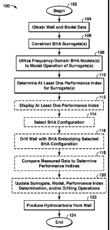
[0035] FIG. 1 is an exemplary flow chart for modeling BHA surrogates;
[0036] FIG. 2 is an exemplary flow chart for modeling BHA surrogates;
[0037] FIG. 3A illustrates a perspective view of a bottom hole assembly;
[0038] FIG. 3B illustrates a cross section of the bottom hole assembly of
FIG. 3A;
[0039] FIGs. 3C and 3D provide schematic illustrations of a beam element
model of a
section of bottom hole assembly;
[0040] FIG. 4 provides a schematic illustration of a beam element model
of a section of
bottom hole assembly;
[0041] FIG. 5 shows an exemplary total BHA sideforce index plot;
[0042] FIG. 6 shows an exemplary sideforce slope index plot;
[0043] FIG. 7 shows an exemplary comparison of two sideforce slope index
plots;
[0044] FIG. 8 provides an exemplary schematic of a modeling system;
[0045] FIG. 9 provides an exemplary screen view provided by a modeling
system;
[0046] FIGs. 10A-10D are exemplary screen views provided by a modeling
system;
[0047] FIGs. 11A-11B are exemplary screen views provided by a modeling
system;
[0048] FIG. 12 provides an exemplary screen view provided by a modeling
system;
[0049] FIG. 13 provides an exemplary screen view provided by a modeling
system;
[0050] FIGs. 14A-14B are exemplary screen views provided by a modeling
system;
- 11 -
CA 02744419 2011-05-20
WO 2010/059295 PCT/US2009/059040
[0051] FIG. 15 provides an exemplary screen view provided by a modeling
system;
[0052] FIG. 16 provides an exemplary screen view provided by a modeling
system;
[0053] FIG. 17 provides an exemplary screen view provided by a modeling
system;
[0054] FIGs. 18A-18B are exemplary screen views provided by a modeling
system;
[0055] FIGs. 19A-19C are exemplary screen views provided by a modeling
system;
[0056] FIGs. 20A-20B are exemplary screen views provided by a modeling
system;
[0057] FIGs. 21A-21E are exemplary screen views provided by a modeling
system;
[0058] FIG. 22 provides a representative flow chart of a batch mode
operation;
[0059] FIGs. 23A-23D are exemplary screen views provided by a modeling
system;
[0060] FIG. 24 provides an exemplary screen view provided by a modeling
system;
[0061] FIG. 25 provides an exemplary screen view provided by a modeling
system to
compare measured data with model results;
[0062] FIG. 26 provides an exemplary screen view of means to control the
output in the
display of FIG. 25; and
[0063] FIG. 27 shows the lateral accelerations of a BHA measured by a near-
bit data
recorder.
DETAILED DESCRIPTION
[0064] In the following detailed description section, the specific
embodiments of the
present techniques are described in connection with preferred embodiments.
However, to the
extent that the following description is specific to a particular embodiment
or a particular use
of the present techniques, this is intended to be for exemplary purposes only
and simply
provides a concise description of the exemplary embodiments. Moreover, to the
extent that a
particular feature or aspect of the present systems and methods are described
in connection
with a particular embodiment or implementation, such features and/or aspects
may similarly
be included or used in connection with other embodiments or implementations
described
herein or otherwise within the scope of the invention claimed in this or
related applications.
Accordingly, the invention is not limited to the specific embodiments
described below, but
rather, it includes all alternatives, modifications, and equivalents falling
within the true scope
of the appended claims.
[0065] The present disclosure is directed to methods and systems for
modeling,
designing, and utilizing bottom hole assemblies to evaluate, analyze, design,
and assist in the
drilling of wells and in the production of hydrocarbons from subsurface
formations. Under
the present techniques, a modeling system may include software or modeling
programs that
characterize the vibration performance of one or more candidate BHA's
graphically in what
- 12 -
CA 02744419 2011-05-20
WO 2010/059295 PCT/US2009/059040
is referred to as "design mode." In some implementations, the vibration
performance of two
or more candidate BI-[A's may be displayed graphically and simultaneously to
facilitate
comparison of the candidate BHA's. The BHA used in a drilling system may be
selected
based on one or more relative vibration performance indices for different BHA
surrogates.
These indices may include point indices, such as an end-point curvature index,
and interval
indices, such as a BHA strain energy index, an average transmitted strain
energy index, a
transmitted strain energy index, a root-mean-square (RMS) BHA sideforce index,
an RMS
BHA torque index, a total BHA sideforce index, a total BHA torque index, a
transmissibility
index, and a sideforce slope index, which are discussed further below, in
addition to specific
static design objectives for the respective assembly.
[0066] Further, the present disclosure provides methods and systems that
utilize a "log
mode" display to compare predicted vibration characteristics with measured
data under
specific operating conditions. The same indices used in the design mode may be
presented in
a log mode display to compare measured drilling data with the indices to
assist in assessing
the BHA vibration performance and to gain an understanding of how to evaluate
the different
vibration performance metrics by comparison with field performance data (e.g.,
measured
data). For example, and as will be better understood from the description
herein, one or more
of the data sets from the design mode, including the vibration performance
indices, may be
compared against measured data and/or data derived from measured data. The
comparison
may reveal helpful information such as the components of the BHA most likely
contributing
to the vibrations, the drilling conditions that will avoid vibrations,
relative contributions of
particular indices, excitation modes, and/or vibrational modes to the actual
performance, and
other information to aid in improving the modeling process, the BHA design
process, and/or
the development of drilling operational plans. Additionally or alternatively,
this same data
may be plotted in a format similar to that used for the vibration performance
indices, with
rotary speed and/or bit weight on the independent axes, showing the
relationships of the
measured data to the vibration performance indices. Since this data is
normally obtained in a
Drilling Vibrations Data Test, this plot is referred to as the "DVDT" display.
[0067] Turning now to the drawings, and referring initially to FIG. 1,
an exemplary
flow chart 100 of a process of modeling and operating a drilling system in
accordance with
certain aspects of the present techniques is described. In this process,
candidate BHA
configurations are represented by surrogates that can be utilized in modeling
programs. The
modeling programs of the present disclosure provide graphical and/or numerical
representations of the how the BHA configuration would operate during
implementations
- 13 -
CA 02744419 2011-05-20
WO 2010/059295 PCT/US2009/059040
under one or more operating conditions. The graphical and/or numerical
representations may
be presented in the form of one or more indices, which may be evaluated on an
absolute or
comparative basis to identify a preferred BHA for given operating conditions
and/or a
preferred set of operating conditions for a given BHA.
[0068] The flow chart begins at block 102. At block 104, data may be
obtained for use
in the methods of the present disclosure. The data may include well operating
parameters
(e.g., weight on bit (WOB) range, rotary speed range (e.g., rotations per
minute (RPM)),
nominal borehole diameter, hole enlargement, hole angle, drilling fluid
density, depth, and
the like). Some model-related parameters may also be obtained, such as the
vibrational
excitation modes to be modeled (specified as integer and/or non-integer
multiples of the
rotary speed and/or specific vibration frequencies), element length, boundary
conditions, and
number of "end-length" elements and the end-length increment value. Then, one
or more
BHA surrogates may be constructed, as shown in block 106. The construction of
the BHA
surrogates includes identifying BHA design parameters (e.g., drill collar
dimensions and
mechanical properties, stabilizer dimensions and locations in the BHA, drill
pipe dimensions,
length, and the like). As will be described more thoroughly below, the BI-IA
surrogate may
be constructed in a variety of suitable manners provided that the surrogate
can be modeled
using frequency-domain models.
[0069] In block 108, the operation of the BHA surrogate is modeled using
one or more
frequency-domain models. The modeling of the BHA surrogates may include
consideration
of the static solutions and the dynamic solutions. The modeling may include
two dimensional
models and/or three dimensional models, both of which are described in better
detail below.
The frequency-domain models provide various data about the operation of the
BHA
surrogate, which can be used to generate at least one vibration performance
index. FIG. 1
illustrates at block 110 the step of determining at least one vibration
performance index for a
BHA surrogate. Examples of illustrative vibration performance indices are
provided below
together with examples of possible uses and interpretations of such indices.
At least one
index is then displayed or otherwise presented to a user or an operator, which
is represented
by block 112 in FIG. 1. The display or presentation of the vibration
performance index may
communicate the index to the user in any suitable manner and in any suitable
format. For
example, the vibration performance index may be presented in numerical and/or
graphical
formats. Additionally, the index may be presented on a computer display, on a
printed page,
transmitted to a remote location for presentation, stored for later retrieval,
etc. With
experience, a BHA design engineer may appreciate the design tradeoffs and, by
comparing
- 14 -
CA 02744419 2011-05-20
WO 2010/059295 PCT/US2009/059040
vibration performance index results for different designs, may develop BHA
designs with
improved operating performance and/or identify better operating parameters. An
example of
the design iteration process is described further below.
[0070] FIG.
1 further illustrates that following the determination and display of a
vibration performance index, various optional steps may be included in the
methods within
the scope of the present disclosure. Once modeled, one of the BHA
configurations
represented by a surrogate may be selected, as shown in block 114. The
selection may be
based on a comparison of multiple BHA surrogates. That is, the modeling of the
BHA
surrogates may include different displays of the calculated state vectors
(e.g., displacement,
tilt, bending moment, lateral shear force of the beam, and BHA/wellbore
contact forces and
torques) as a function of the operating parameters (e.g., RPM, WOB, etc.),
distance to the bit,
and BHA configuration. The
displayed results or solutions, including the vibration
performance indices, may include detailed 3-dimensional state vector plots
intended to
illustrate the vibrational tendencies of alternative BHA configurations. The
selection of a
BHA configuration may include selecting a preferred BHA configuration in
addition to
identifying a preferred operating range for the preferred configuration. The
selection may be
based on the relative and/or absolute performance of the BHA configurations,
which may be
evaluated using a variety of indices, including end-point curvature index, BHA
strain energy
index, average transmitted strain energy index, transmitted strain energy
index, RNIS BHA
sideforce index, RMS BHA torque index, total BHA sideforce index, total BHA
torque index,
transmissibility index, sideforce slope index, and any mathematical
combination thereof. In
some implementations, the selection of a BHA configuration may include the
selection of a
configuration that had been represented by one or more of the BHA surrogates.
Additionally
or alternatively, the selected BHA configuration may incorporate features or
aspects from
two or more of the BHA surrogates.
[0071]
Continuing with the schematic flow chart 100 of FIG. 1, the methods of the
present disclosure may optionally include drilling a well with a bottom hole
assembly
embodying the selected BHA configuration, such as represented by block 116.
The drilling
of the well may include forming the well to access a subsurface formation with
the drilling
equipment.
100721 In
some implementations, measured data may then be compared with calculated
data and/or determined vibration performance indices for the selected BHA
configuration, as
shown in block 118. That is, as the drilling operations are being performed or
at some time
period following the drilling operations, sensors may be used to collect
measured data
- 15 -
CA 02744419 2011-05-20
WO 2010/059295 PCT/US2009/059040
associated with the operation of the drilling equipment. For example, the
measured data may
include but is not limited to RPM, WOB, axial, lateral, and stick/slip
vibration measurements,
drilling performance as determined by the Mechanical Specific Energy (MSE), or
other
appropriate derived quantities. Downhole data may be either transmitted to the
surface in
real-time or it may be stored in the downhole equipment and received when the
equipment
returns to the surface. The measured data and/or data derived from the
measured data may be
compared with calculated data and/or vibration performance indices from the
modeling
system for the selected BHA configuration.
[0073] The comparison of the measured data (or data derived from the
measured data)
with the model data and vibration performance indices can be used in a variety
of manners,
some examples of which are described in more detail herein. An illustrative
and non-
exhaustive list of such uses includes 1) updating the surrogate to better
represent the BHA
configuration; 2) updating the frequency-domain model to better simulate the
response of the
BHA during drilling operations under a variety of conditions; 3) updating the
calculations
and/or parameters used to determine one or more vibration performance indices;
4) updating
the drilling operations plans for a selected bottom hole assembly
configuration, such as
represented by box 120 in FIG. 1; and 5) using measured vibration data to
determine the
model input excitation, simulating the response of the surrogates with this
input, and
comparing the model results with other measured data that is considered to be
the system
output response. The feedback process facilitates modeling validation and
verification. It
also helps to determine which of the vibration performance indices warrant
greater weighting
in the BHA configuration selection process, thus providing learning aids to
advance the
development of the BHA configuration selection process. Additionally or
alternatively, the
comparison between the model results and the measurements may enable the
vibration
performance indices to more accurately predict or indicate the vibrational
tendencies of a
BHA surrogate, such as by allowing one or more input parameters of a vibration
performance
index to be further refined or tuned. One example of such vibration
performance index
improvements includes weighting the various vibrational excitation modes to
more accurately
consider the modes that are most relevant.
[0074] Once the wellbore is formed, hydrocarbons may be produced from the
well, as
shown in block 122. The production of hydrocarbons may include completing the
well with a
well completion, coupling tubing between the well completion and surface
facilities, and/or
other known methods for extracting hydrocarbons from a wellbore. The process
ends at
block 124.
- 16 -
CA 02744419 2011-05-20
WO 2010/059295 PCT/US2009/059040
[0075] Beneficially, the present techniques may be utilized to design,
construct, and/or
utilize equipment that can reduce the impact of limiters that may hinder
drilling operations.
In some implementations, two or more BHA configurations may be compared
simultaneously
with concurrent calculation and display of model results for two or more
surrogates. With
this comparison, the merits of alternative BHA configurations can be
evaluated. Further, in
implementations where the calculated model data and the measured data are
associated with
the selected BHA configuration, other limiters that may be present during the
drilling of the
wellbore may be identified and addressed in a timely manner to further enhance
drilling
operations. For example, if the primary limiter appears to be torsional
stick/slip vibrations
and the sources of torque in the BHA due to contact forces have been
minimized, another
possible mitigator is to choose a less aggressive bit that generates less
torque for a given
applied weight on bit. An example of the modeling of two or more BHA
configuration
surrogates is described in greater detail below in FIG. 2.
[0076] FIG. 2 is an exemplary flow chart 200 of the modeling of two or
more BHA
surrogates in accordance with certain aspects of the present techniques. For
exemplary
purposes, in this flow chart, the modeling of the two or more BHA surrogates
is described as
being performed by a modeling system. The modeling system may include a
computer
system that operates a modeling program. The modeling program may include
computer
readable instructions or code that compares two or more BHA surrogates, which
is discussed
further below. While FIG. 2 is directed to the comparison of two or more BHA
surrogates,
the present methods and systems are useful in modeling a single BHA surrogate
to identify
operational and/or design parameters that can be modified to improve
performance by
reducing vibrations.
[0077] The flow chart 200 begins at block 202. To begin, the BHA layout
and
operating parameters are obtained for use in the modeling operations
introduced above. At
block 204, operating parameters may be obtained. The operating parameters,
such as the
anticipated ranges of WOB, RPM and wellbore inclination, may be obtained from
a user
entering the operating parameters into the modeling system or accessing a file
having the
operating parameters. For the static model, the condition of the BHA model end-
point (e.g.,
end away from the drill bit) can be set to either a centered condition (e.g.,
the pipe is centered
in the wellbore) or an offset condition (e.g., the pipe is laying on the low
side of the
wellbore).
[0078] The BHA design parameters are then obtained, as shown in block
206. The
BHA design parameters may include available drill collar dimensions and
mechanical
- 17 -
CA 02744419 2011-05-20
WO 2010/059295 PCT/US2009/059040
properties, dimensions of available stabilizers, drill pipe dimensions,
length, and the like. For
example, if the drilling equipment is a section of tubing or pipe, the BHA
design parameters
may include the inner diameter (ID), outer diameter (OD), length and bending
moment of
inertia of the pipe, and the pipe material properties. Also, the modeling
system may model
drilling equipment made of steel, non-magnetic material, Monel, aluminum,
titanium, etc. If
the drilling equipment is a stabilizer or under-reamer, the BHA design
parameters may
include blade OD, blade length, and/or distance to the blades from the ends.
[0079] At block 208, the initial BHA surrogates are obtained. Obtaining
of the BHA
surrogates may include accessing a stored version of a previously modeled or
utilized BHA
configuration or BHA surrogate, interacting with the modeling system to
specify or create a
BHA surrogate from the BHA design parameters, or entering a proposed BHA
configuration
into the model that was provided by the drilling engineer or drilling service
provider. The
BHA surrogates specify the positioning of the equipment and types of equipment
in the BHA,
usually determined as the distance to the bit of each component.
[0080] Once the different BHA surrogates are obtained and/or constructed,
the results
for the selected BHA surrogates are calculated/modeled, as shown in block 210.
The
calculations may include calculation of the static states to determine force
and tilt angle at the
bit and static stabilizer contact forces, calculation of dynamic vibration
performance indices,
calculation of dynamic state values for specific excitation modes as a
function of rotary
speed, weight on bit, and distance to bit, and the like. More specifically,
the calculations may
include the dynamic lateral bending (e.g., flexural mode) and eccentric whirl
dynamic
response as perturbations about a static equilibrium, which may be calculated
using the State
Transfer Matrix method described below or other suitable method. This flexural
or dynamic
lateral bending mode may be referred to as "whirl." The static responses may
include the
state vector response (e.g., displacement, tilt, bending moment, shear force,
and contact
forces or torques) as a function of distance from the bit, WOB, fluid density,
and wellbore
inclination (e.g., angle or tilt angle). For the dynamic response values, the
state variables
may be calculated as a function of distance from the drill bit, WOB, RPM,
excitation mode,
and end-lengths. For the lateral bending and eccentric whirl, the model states
(e.g.,
displacement, tilt, bending moment, shear force, and contact forces or
torques) may be
calculated and displayed as functions of distance from the bit for specified
WOB, RPM,
excitation mode, and end-length.
[0081] As used herein, the "excitation mode" is the integer and/or non-
integer multiple
of the rotary speed or specific excitation frequency at which the system is
being excited (for
- 18 -
CA 02744419 2011-05-20
WO 2010/059295 PCT/US2009/059040
example, it is well known that a roller cone bit provides a three times
multiple axial
excitation, which may couple to the lateral mode). The "end-length" is the
length of pipe
added to the top of the BHA, often in the heavy-weight drillpipe, to evaluate
the vibrational
energy being transmitted uphole. Because the response may be sensitive to the
location of
the last nodal point, one computational approach is to evaluate a number of
such possible
locations for this nodal point for the purpose of computing the response. Then
these different
results may be averaged (by root-mean-square (RMS) or another averaging
method) to obtain
the overall system response for the parametric set of the various excitation
modes and end-
lengths for each RPM and WOB. Additionally or alternatively, the "worst case"
maximum
value may also be presented, which is described further below.
[0082] Once
the results are calculated, the results are displayed as shown in block 210.
When the present methods are implemented for direct comparison of two or more
BHA
surrogates, the results may be displayed simultaneously on one or more display
screens
and/or windows or may be displayed in a common window. As described above, the
results
may similarly be transmitted to remote locations for display or stored for
later retrieval. The
display may be on a screen or other audiovisual medium or may be printed.
Additionally, the
display may include graphical and/or numerical representations of the results.
[0083]
Continuing with the flow chart of FIG. 2, the results are verified, as shown
in
block 212. The
calculation result verification process may include determining by
examination that, for example, there were no numerical problems encountered in
the
simulation and that all excitation modes were adequately simulated throughout
the requested
range of rotary speeds, bit weights, and end-lengths. In some implementations,
the
calculation result verification process may include discarding and/or
discounting numerically
divergent results in calculating one or more vibration performance indices.
Other methods of
verifying the results may be implemented.
[0084] At
block 214, FIG. 2 illustrates that a determination may be made whether the
BHA configurations represented by the surrogates and/or other parameters are
to be
modified. If the BHA configurations or specific parameters are to be modified,
the BHA
configurations and/or parameters may be modified in block 216. The
modifications may
include changing specific aspects in the operating parameters, BHA surrogates,
BHA design
parameters and/or adding a new BHA surrogate. As a specific example, the WOB,
RPM
and/or excitation mode may be changed to model another set of operating
conditions. The
BHA configurations and corresponding surrogates are typically adjusted by
altering the
distance between points of stabilization, by changing the sizes or number of
stabilizers and
- 19 -
CA 02744419 2011-05-20
WO 2010/059295 PCT/US2009/059040
drill collars, by relocating under-reamers or cross-overs to a different
position in the BHA
surrogate, and the like. Once the modifications are complete, the results may
be recalculated
in block 210, and the process may be iterated to further enhance performance.
[0085] However, if the BHA configurations and/or parameters are not to
be modified,
the results are provided, as shown in block 218. Providing the results may
include storing the
results in memory, printing a report of the results, and/or displaying the
results on a monitor.
For example, a side-by-side graphical comparison of selected BHA surrogates
and/or
preferred operating parameters may be displayed by the modeling system. The
results of one
or more of the calculated static and dynamic responses for specified WOB, RPM,
excitation
mode, end-lengths, and vibration indices may be displayed on two-dimensional
or three-
dimensional plots. Similarly, the results may be displayed as results for a
single BHA
surrogate, a comparison of results for two or more BHA surrogates, and/or a
comparison of
modeling results and measured data during actual drilling operations. While
FIG. 2
illustrates that the method ends at block 220, additional steps may follow,
such as the
implementation of drilling operations incorporating the information learned
during the
methods of FIG. 2.
[0086] Beneficially, the modeling of the BHA surrogates may enhance
drilling
operations by providing a BHA more suitable to the drilling environment. For
example, if
one of the BHA surrogates is based on drilling equipment utilized in a certain
field, then
other surrogates may be modeled and directly compared with the previously
utilized BHA
surrogate. That is, one of the BHA surrogates may be used as a benchmark for
comparing the
vibration tendencies of other BHA surrogates. In this manner, the BHA
surrogates may be
compared, either simultaneously or as additional surrogates are modeled, to
determine a BHA
surrogate that reduces the effect of limiters, such as vibrations. To the
extent that the
modeling system is adapted to compare more than two different BHA surrogates,
additional
proposed BHA surrogates can be compared against each other or against a
baseline surrogate.
The comparative approach may be found to be more practical in some
implementations. The
relevant question to answer for the drilling engineer relates to which
configuration of BHA
components operates with the lowest vibrations over the operating conditions
for a particular
drilling operation. A preferred approach to address this design question is to
model several
alternative configurations and then select the one that performs in an optimal
manner over the
expected operating range or to operate the selected configuration at operating
parameters
suggested by the present methods. Such approach can be accomplished
iteratively or through
direct and simultaneous comparison of the several configurations.
- 20 -
CA 02744419 2011-05-20
WO 2010/059295 PCT/US2009/059040
EXEMPLARY BHA SURROGATES
[0087] As described above, BHA surrogates are representations of actual
BHA
configurations that can be input into the modeling systems to simulate the
operation or
response of the represented BHA configuration in a drilling operation.
Accordingly, BHA
surrogates, as representations of actual equipment, incorporate one or more
assumptions
and/or simplifications to allow the equipment to be mathematically modeled. As
with most
mathematical representations of actual equipment, the representation can be
constructed in a
variety of manners, some of which may be different but equal in application.
Similarly, some
of the different surrogate construction techniques may result in different
surrogates that are
more or less appropriate for different uses.
[0088] The present methods encompass the use of any suitable surrogate
that can be
used in a frequency-domain model of drilling operations to simulate drilling
and associated
vibrations. Exemplary surrogates include a lumped parameter surrogate and a
distributed
mass surrogate. In a lumped parameter surrogate, the BHA configuration is
represented by
point masses connected by massless beam and damper elements. In a distributed
mass
surrogate, the BHA configuration is represented by a beam having a distributed
mass.
Depending on the manner in which the BHA surrogate is constructed, the
frequency-domain
model(s) used to model the operation of the surrogate may vary, such as the
selection of a 2D
or a 3D frequency-domain model.
[0089] As suggested above, the BHA surrogates may be constructed in a
variety of
manners and the frequency-domain models may vary within the scope of the
present
disclosure. Through implementation of the present methods, it may be
determined that one
type of surrogate and/or one type of frequency-domain model more accurately
represents
actual drilling operations for a particular BHA configuration, for particular
operating
conditions, or for particular environments. For example, it may be found that
2D lumped
parameter surrogates and associated modeling results correspond sufficiently
closely to
measured data for a particular BHA configuration or drilling application. As
another
example, it may be found that 3D distributed mass surrogates and associated
frequency-
domain modeling results more closely correspond to measured data for a
particular type of
vibration or for a particular excitation mode. Accordingly, methods within the
scope of the
present disclosure include methods where different BHA surrogates and
different frequency-
domain models are used to represent one or more BHA configurations in a single
drilling
operation. Additionally or alternatively, mathematical combinations of
different surrogates
- 21 -
CA 02744419 2011-05-20
WO 2010/059295 PCT/US2009/059040
and/or frequency-domain models may be used to improve the accuracy of the
modeling
results as compared to measured data.
EXEMPLARY LUMPED PARAMETER BHA VIBRATION MODELS
[0090] As
an example, one exemplary implementation of a BHA vibration model is
described. However, it should be noted that other BHA models, for example
using one or
more of the calculation methods discussed above, may also be used to form a
comparative
vibration performance index in a similar manner. As used herein, "BHA
vibration model"
refers to the use of a BI IA surrogate and associated frequency-domain
modeling principles to
model or simulate the vibrations of a drilling operation using the BHA
configuration
represented by the BHA surrogate. These methods may include but are not
limited to two-
dimensional or three-dimensional finite element modeling methods. For example,
calculating
the results for one or more BHA configurations may include generating a
surrogate or
mathematical model for each BHA configuration; calculating the results of the
surrogate for
specified operating parameters and boundary conditions; identifying the
displacements, tilt
angle (first spatial derivative of displacement), bending moment (calculated
from the second
spatial derivative of displacement), and beam shear force (calculated from the
third spatial
derivative of displacement) from the results of the surrogate simulation; and
determining state
vectors and matrices from the identified outputs of the surrogate simulation.
In more
complex models, these state vectors may be assigned at specific reference
nodes, for example
at the neutral axis of the BHA cross-section, distributed on the cross-section
and along the
length of the BHA, or at other convenient reference locations. As such, the
state vector
response data, calculated from the finite element model results, may then be
used to calculate
vibration performance indices to evaluate BHA configurations and to compare
with
alternative BHA configurations, as described herein.
[0091] The BHA
vibration model described in this section is a lumped parameter
model, which is one embodiment of a mathematical model, implemented within the
framework of state vectors and transfer function matrices. The state vector
represents a
complete description of the BHA system response at any given position in the
BHA
surrogate, which is usually defined relative to the location of the bit. The
transfer function
matrix relates the value of the state vector at one location with the value of
the state vector at
some other location. The total system state includes a static solution plus a
dynamic
perturbation about the static state. The linear nature of the model for small
dynamic
perturbations facilitates static versus dynamic decomposition of the system.
The dynamic
model presented in this section is one variety in the class of forced
frequency response
- 22 -
CA 02744419 2011-05-20
WO 2010/059295 PCT/US2009/059040
models, with specific matrices and boundary conditions as described below.
Other dynamic
models may be developed for BHA vibration models utilizing alternative BI-[A
surrogates
and/or alternative operating parameters.
[0092]
Transfer function matrices may be multiplied to determine the response across
a
series of elements in the model. Thus, a single transfer function can be used
to describe the
dynamic response between any two points. A lumped parameter model yields an
approximation to the response of a continuous system. Discrete point masses in
the BHA
surrogate are connected by massless springs and/or dampers to other BHA
surrogate mass
elements and, in one variation, to the wellbore at points of contact by
springs and, optionally,
damper elements. The masses are free to move laterally within the constraints
of the applied
loads, including gravity.
MATRIX AND STATE VECTOR FORMULATION
[0093] For
lateral motion of a lumped parameter model in a plane, the state vector
includes the lateral and angular deflections, as well as the beam bending
moment and shear
load. The state vector u is extended by a unity constant to allow the matrix
equations to
include a constant term in each equation that is represented. The state vector
u may then be
written as equation (el) as follows:
u = M (el)
V
1
Where y is lateral deflection of the beam from the centerline of the assembly,
9 is the angular
deflection or first spatial derivative of the displacement, M is the bending
moment that is
calculated from the second spatial derivative of the displacement, and V is
the shear load of
the beam that is calculated from the third spatial derivative of the
displacement. For a three-
dimensional model, the state vector defined by equation (el) may be augmented
by additional
states to represent the displacements and derivatives along an orthogonal axis
at each node.
The interactions between the motions at each node may, in the general case,
include coupled
terms.
[0094] By
linearity, the total response may be decomposed into a static component us
and a dynamic component lid (e.g., u = u + lid).
- 23 -
CA 02744419 2011-05-20
WO 2010/059295 PCT/US2009/059040
[0095] In
the forced-frequency response methods, the system is assumed to oscillate at
the frequency co of the forced input, which is a characteristic of linear
systems. Then, time
and space separate in the dynamic response and, using superposition, the total
displacement
of the beam at any axial point x for any time t may be expressed by the
equation (e2):
u(x, t) = us (x) + u(x)sin(cot) (e2)
[0096]
State vectors u, (for element index i ranging from 1 to N) may be used to
represent the state of each mass element, and the state vector uo is used to
designate the state
at the bit. Transfer function matrices are used to relate the state vector u,
of one mass
element to the state u,_, of the preceding mass element. If there is no
damping in the model,
then the state vectors are real-valued. However, damping may be introduced and
then the
state vectors may be complex-valued, with no loss of generality.
[0097]
Because state vectors are used to represent the masses, each mass may be
assumed to have an associated spring and/or damper connecting it to the
preceding mass in
the model. With the notation M, denoting a mass transfer matrix, and a beam
bending
element transfer matrix represented by Bõ the combined transfer function T, is
shown by the
equation (e3) below.
T, = M,B, (e3)
Numerical subscripts are used to specify each mass-beam element pair. For
example, the
state vector u1 may be calculated from the state u0 represented by the
equation (e4).
u, = M,B,u, TA), and thus u, =- T,u, (e4)
These matrices can be cascaded to proceed up the BHA to successive locations.
For
example, the state vector u2 may be represented by the equation (e5).
u2 = T2141 = T2T1u0 (e5)
While continuing up to a contact point, the state vector UN may be represented
by equation
(e6).
=- TN-1 = TNTN-1 '..T1u0 (e6)
[0098]
Accordingly, within an interval between contact points, the state uj at any
mass
element can be written in terms of any state below that element u, using a
cascaded matrix Su
times the appropriate state vector by the equation (e7):
uj = Su u, where for i < j, Su = T (e7)
Consideration of the state vector solution at the contact points will be
discussed below.
- 24 -
CA 02744419 2011-05-20
WO 2010/059295
PCT/US2009/059040
FORMULATION OF MASS MATRICES
[0099] The
mass transfer function matrix for the static problem is derived from the
balance of forces acting on a mass element m. Generally, each component of the
BHA is
subdivided into small elements, and this lumped mass element is subjected to
beam shear
loads, gravitational loading (assuming inclination angle 0 ), wellbore contact
with a stiffness
k, and damping force with coefficient b. The general force balance for the
element may be
written as equation (e8) using the "dot" and "double dot" notations to
represent the first and
second time derivatives, or velocity and acceleration, respectively.
mj) = V, ¨ ¨ mg sin 0 ¨ ky ¨ by = 0 (e8)
[0100] The
lumped mass element transfer function matrix under static loading
includes the lateral component of gravity (mg sin0) and either a contact
spring force or,
alternatively, a constraint applied in the solution process, in which case the
value of k is zero.
In the static case, the time derivatives are zero, and thus inertial and
damping forces are
absent. The static mass matrix may be written as the following equation (e9).
( 1 0 0 0 0
0 1 0 0 0
M s = 0 0 1 0 0 (e9)
k 0 0 1 (mg sin 0)
0 0 0 0 1
[0101] In
lateral dynamic bending, the forces applied to the mass consist of the beam
shear forces, wellbore contact, and damping loads. Again, the wellbore contact
may be either
the result of a spring force or an applied constraint relation. However,
because the dynamic
perturbation about the static state is sought (using the principle of linear
superposition), the
gravitational force is absent from the dynamic mass matrix.
[0102] In
the dynamic example, the applied loads may be unbalanced, leading to an
acceleration of the mass element. The mass times lateral acceleration equals
the force
balance of the net shear load, spring contact, and damping forces, resulting
in the equation
(e 1 0).
mi) kY b.3> (e 1 0)
Assuming a complex harmonic forced response yd e", where i represents the
imaginary
number equal to V-1 , the solution to equation (e10) may be found in equation
(ell).
- 25 -
CA 02744419 2011-05-20
WO 2010/059295 PCT/US2009/059040
V, = V, + (k + ibc o ¨ mcp2) (e I I)
[0103] The
lumped mass element transfer function matrix MB, for the lateral bending
mode dynamic perturbation, is then written by the following equation (e12).
( 1 0 0 0 0\
0 1 0 0 0
MB= 0 0 1 0 0
(e12)
(k + ibco ¨ mco2) 0 0 1 0
0 0 0 0 1
[0104] The mass matrix in the dynamic whirl model involves a constant-
magnitude
force which resembles the gravitational force in the static mass matrix. It is
assumed that
each drill collar has a slightly unbalanced mass, generating a centrifugal
force proportional to
this unbalanced mass times the square of the rotational frequency. For a small
value c which
represents the dimensionless off-axis distance of the unbalanced mass, the
equation of motion
for forced response is given by equation (e13).
n2.)) = V, ¨ + crimp' ¨ ky ¨ bY
(e13)
[0105] The
radial displacement does not change with time for this simplified whirl
mode example, and thus the acceleration and velocity may be set to zero. This
represents a
steady rotational motion, not unlike a rotating gravitational load, in
contrast to the lateral
bending mode in which the displacement oscillates through a zero value. The
resulting whirl
matrix is represented in equation (e14).
(1 0 0 0 0 \
0 1 0 0 0
M= 0 0 1 0 0 (e14)
k 0 0 1 (ono')
0 0 0 0 1
[0106] The
value c may take either positive or negative signs in order to represent
the shape of the whirl response being modeled. The first whirl mode is
generally represented
by alternating signs on successive intervals of BHA components as one proceeds
up the
borehole.
[0107] The
lumped parameter mass m is defined as the mass of the element piece of
the respective BHA component. In addition, the mass of the drill collar, pipe,
or other BHA
component is effectively increased by the drilling fluid contained within the
collar and that
which is entrained by the BHA element as it vibrates. The technique of "added
mass" may be
used to approximate this phenomenon. For this purpose, a crude approximation
is to increase
- 26 -
CA 02744419 2011-05-20
WO 2010/059295 PCT/US2009/059040
the dynamic collar mass by 10%, leading to a slight reduction in natural
frequency. This is a
representative value only, and calibration of model results with field data
may indicate
alternative values for the "added mass" effect that may be used in the model.
Note that it is
not appropriate to apply the added mass to the static solution. As noted
above, depending on
the solution method, the spring constant may be omitted if the solution is to
apply a constraint
relationship such that the BHA model is not permitted to extend outside the
wellbore by more
than a very small amount.
[0108] If
the constraint model is not used, then the contact stiffness k in the above
relations should be included explicitly. In this example, a factor to be
considered in the
lo choice
of wellbore contact stiffness k when modeling dynamic excitation is that the
value of
k should be chosen sufficiently high for the mass m such that the natural
frequency Vichn is
greater than the maximum excitation frequency co to be evaluated, so that
resonance due to
this contact representation is avoided. Thus, for an excitation mode of n
times the rotary
speed, the contact stiffness k may be greater than m(nco)2 (e.g., k > m(n
co)2).
[0109] Alternatively, and in the preferred embodiment, compliance at the
points of
contact between BHA and wellbore may be neglected and a fixed constraint
relationship
applied in the solution method, with k = 0 in the matrices above. This
approach is described
further below.
FORMULATION OF STIFFNESS MATRIX
[01101 The Euler-Bernoulli beam bending equation for a uniform beam with
constant
Young's modulus E, bending moment of inertia I, and axial loading P may be
written as the
fourth-order partial differential equation (e15).
84, 82,
EI __________________________________ P __ =O
(e15)
ax4 ax 2
[0111] The
characteristic equation for the general solution is represented by equation
(e16)
y eflx
(e16)
This equation expresses the lateral displacement as the exponential power of a
parameter fi
times the distance x from a reference point, in which the term is to be
found by replacing
this solution in equation (e15) and solving with equations (e17) and (e18)
below.
- 27 -
CA 02744419 2011-05-20
WO 2010/059295 PCT/US2009/059040
2 2 P
(16 EI)= 0 (e17)
p ,o, 11¨P (e
18)
EI
[0112] Note
that p is either real (beam in tension), imaginary (beam in compression),
or 0 (no axial loading). The appropriate particular solution is a constant
plus linear term in X.
Thus, the displacement of an axially loaded beam may be represented by the
equation (e19).
y = a + bx + ce14' + de-13' (e19)
where the constants a, b, c, and d are found by satisfying the boundary
conditions.
[0113] The remaining components of the state vector are determined by
the following
equations in the spatial derivatives of lateral displacement with the axial
coordinate x (e20).
aya 3
9= ¨ M EIa2y
(e20)
ax 8x2 V = EIy 0x3
[0114] The
resulting beam bending stiffness transfer function matrix B may be
represented by the following equation (e21).
(
(
1 L - 2 + + t 2,8L- +e
________________________________________________________ 0
2P 2P
0 1 0
213E1 2P
B =- + e-fiL (e21)
0 0 0
2 2/3
( + e-x\
r ¨ flefiL fle-fiL
0 0 0
2 2
0 0 0 0 1
BOUNDARY CONDITIONS AND SYSTEM EXCITATION
[0115] With the mass and beam element transfer functions defined, the
boundary
conditions and system excitation are determined to generate frequency-domain
model
predictions. Separate boundary conditions are used to model the static
bending, dynamic
lateral bending, and eccentric whirl problems.
[0116] In
each of these examples of lumped parameter BHA vibration models, the
solution proceeds from the bit to the first stabilizer or other contact point,
then from the first
stabilizer to the second stabilizer or other contact point, and so on,
proceeding uphole one
solution interval at a time (e.g., from the bit as the starting interval).
Finally, the interval
from the top contact point to the end point is solved. As suggested, contact
points are often
provided by stabilizers, but may be provided by other BHA components, such as
an under-
- 28 -
CA 02744419 2011-05-20
WO 2010/059295 PCT/US2009/059040
reamer, or perhaps even by contact of one or more BHA components at
intermediate points
between specific contact points, such as drill collars resting on the wall
between stabilizers.
For convenience and brevity herein, the exemplary stabilizer will be used to
refer to the
variety of BHA components that may provide a contact point. The end point is
the upper
node of the BHA model, and it may be varied to consider different possible
nodal points at
the "end-length." An appropriate lateral displacement for this end point is
assumed in the
static model, based on the amount of clearance between the pipe and the
wellbore.
[0117] In
these methods, the states in each solution interval are determined by three
conditions at the lower element (bit or bottom stabilizer in the interval),
and one condition at
the upper element (end point or top stabilizer in the interval). With these
four conditions and
the overall matrix transfer function from the lower to the upper element, the
remaining
unknown states at the lower element may be calculated.
[0118]
Beginning at the bit, the displacement of the first stabilizer is used to
determine the bit state, and thus all states up to the first stabilizer are
determined using the
appropriate transfer function matrices. By continuity, the displacement, tilt,
and moment are
now determined at the first stabilizer point of contact. The beam shear load
is undetermined,
as this state does not have a continuity constraint because there is an
unknown side force
acting between the stabilizer and the wellbore. The displacement of the next
stabilizer is used
to provide the fourth condition necessary to obtain the solution over the next
interval, and
thus the complete state at the stabilizer is determined. The contact force
between stabilizer
and wellbore may be calculated as the difference between this state value and
the prior shear
load calculation from the previous BHA section. Using the cascaded matrix
formulation in
equation (e22).
r
Y Y ,
0 0,
f V, = unknown
M1 = S M with the conditions
(e22)
y -= 0
V
1
1 1
Then the unknown shear load at the lower stabilizer is calculated using an
equation (e23) to
obtain zero displacement at the upper position.
0 = S,,y, + S120, + S13M1 + Si, V, + S15
(e23)
[0119] The
beam shear load is discontinuous across the contact points, and the
sideforce at such a node may be calculated as the difference between the value
obtained by
propagating the states from below, V, and the value calculated to satisfy the
constraint
- 29 -
CA 02744419 2011-05-20
WO 2010/059295 PCT/US2009/059040
relation for the next segment, V, . Therefore, the contact sideforce may be
represented by
the equation (e24).
(e24)
[0120] For
the static example, the tilt and sideforce are unknown at the bit. A trial bit
tilt angle is used to generate a response and the state vectors are propagated
uphole from one
contact point to the next, finally reaching the end-point. The final value for
the bit tilt angle
and sideforce are determined by iterating until the appropriate end condition
is reached at the
top of the model, for instance a condition of tangency between the pipe and
borehole wall.
Alternatively, the solution may start at an uphole point of tangency and
proceed downhole to
the bit, iterating to convergence on the bit condition by varying the distance
to the point of
tangency. Other convergence methods may also be selected.
[0121]
Additionally or alternatively, the stabilizer configuration or the
configuration
of another element of the BHA surrogate may suggest an additional constraint.
For example,
for full-gauge stabilizers, it may be appropriate to further constrain the BHA
vibration model
to a tilt angle of zero. Such a constraint may be appropriate due to the
interactions between
the full-gauge stabilizers and the wellbore wall. A BHA vibration model
incorporating this
additional constraint will result in an increase in the reaction sideforces in
the model and a
discontinuity in the bending moment will occur to represent the reaction
torque due to the
fixed tilt angle constraint. Additionally, equation (e22) above will be
modified with the
additional constraint as equation (e22') for the node/ where the tilt
constraint applies.
r
,
y=o
(9j 0,
8=0
M = S M with the conditions (e22')
M unknown
V V.
V. unknown
1 1
[0122] For
the dynamic models (flexural bending, whirl, and twirl), a reference bit
excitation sideforce is applied, e.g., Vim = const . The first stabilizer is
assumed to be
constrained by the pinned condition (e22) or by the built-in condition (e22').
If applying
(e22), two more conditions are specified to uniquely solve the equations from
the bit up to the
first stabilizer. One choice for the boundary conditions is to assume that for
small lateral
motion, the tilt and moment at the bit are zero. This set of boundary
conditions may be
written as shown in equation (e25):
- 30 -
CA 02744419 2011-05-20
WO 2010/059295
PCT/US2009/059040
Y stab = bit = M bit ¨ O Vb, = const (e25)
[0123] An
alternate set of boundary conditions may be considered by assuming that
the tilt angle at the first stabilizer is zero as in (e22 '), equivalent to a
cantilevered condition.
One selection for the remaining constraint is to assume that there is no
moment at the bit.
This alternate set of boundary conditions may be written as shown in equation
(e26):
Y stab = stab ¨ M bit =13 Vb, const (e26)
[0124] As is
well understood, the bit may be excited in a variety of manners leading
to dynamic vibrations. The bit excitation by way of an applied sideforce
described above is
one common manner. The present methods may be adapted to provide BHA vibration
models for other forms of bit excitation as well. As one exemplary
modification to
accommodate or consider an alternative form of bit excitation, the bit may be
excited by an
applied moment at the bit, such as may occur in drilling operations when the
bit is penetrating
a laminated formation. The BHA vibration model may be run utilizing an applied
excitation
frequency for an applied moment at the bit at any multiple of the rotary
speed. In some
implementations, it may be preferred to run the model multiple times utilizing
various
multiples of the rotary speed and considering averages, maximums, and/or
historical/measured data to provide a more robust and/or accurate model. For
example, while
a 1X multiple of the rotary speed may be the most likely excitation frequency,
the model may
be run using various multiples, including non-integer multiples such as 1.5X,
1.75X, etc.
Additionally and alternatively, a fixed excitation frequency can be applied to
the bit to
represent certain excitation sources that are constant in frequency and not
multiples of the
rotary speed. One example is the drilling fluid pressure which has pressure
pulses in
accordance with the stroke rate of the mud pumps. These pulses may cause
lateral motion at
the bit due to the time-varying pressure drop through the bit nozzles.
Y stab = Yb,, Vba = (1) Mb, = const (e25')
Y stab = slab = Vba = O Mbit = const (e26)
[0126]
Regardless of the form of excitation applied, which may include one or more
of those described above and/or other common excitations, the solution marches
uphole one
-31 -
CA 02744419 2011-05-20
WO 2010/059295
PCT/US2009/059040
stabilizer at a time. The solution, or rather the implementation of the model,
terminates at the
last node of the BHA surrogate, which is arbitrarily chosen but may be located
at different
"end-lengths" in the dynamic case. By selecting different end-lengths and RMS-
averaging
the results, vibration performance indices may be formed that are robust. To
guard against
strong resonance at an individual nodal point, the maximum result may be
examined as well,
and conversely, the minimum value may be examined to evaluate possible
preferred
operating regions. These techniques of RMS-averaging and examining the maximum
may be
preferred when determining a vibration performance index that is sensitive to
the selection of
a nodal point location. For example, an end-point curvature index and other
point indices
may be more sensitive to nodal point locations than the interval indices
described herein.
Being less sensitive to the end location and condition, the interval indices
may be preferred in
some implementations. It should further be noted, as indicated above, that BHA
contact with
the borehole at locations between stabilizers may optionally be treated as a
nodal point in this
analysis method, and the solution propagation modified accordingly.
EXEMPLARY DISTRIBUTED MASS BHA VIBRATION MODELS
[0127] As
introduced above, bottom hole assemblies can be represented by surrogates
of a variety of construction methods. The exemplary model described above
considered a
lumped parameter BHA vibration model in great detail. As an illustration of
other BHA
surrogates and associated frequency-domain models that may be used in BHA
vibration
models within the scope of the present disclosure, an exemplary distributed
mass BHA
vibration model will now be described with reference to the discussions above.
[0128] As
with the discussion above, the system state vector for a distributed mass
BHA vibration model is written as equation (e27):
( Y (lateral deflection\
angular deflection
u = M = bending moment
(e27)
V shear load
\ unity constant
1
\
By linearity, the total response may be decomposed into static and dynamic
components. In
the forced-frequency response method, the system is assumed to oscillate at
the frequency of
the forced input; this is a characteristic of linear systems. Then time and
space separate in the
dynamic response, and, using superposition, one may write the state vector as
a function of
time and space as equation (e28):
- 32 -
CA 02744419 2011-05-20
WO 2010/059295
PCT/US2009/059040
u(x, t) us (x)+ ud (X) sin(rot) (e28)
[0129]
While many of the principles from the above lumped parameter discussion are
relevant to this distributed mass example, several of the factors and
relationships described
above depended on the mass of the BHA as represented in the surrogates. As the
distributed
mass BHA surrogate does not simplify the BHA configuration as point mass and
springs
and/or dampers, several of the relationships described above are adapted to
correspond with
the construction of the BHA surrogate, as will be seen below. The relations to
describe the
beam deflections depend on the beam properties (E and /) and the distributed
weight per unit
length, W. The axial load, P, is also a factor that translates directly from
the lumped
parameter model to the distributed mass model. As with the above example, the
present
example will consider both the static case and the dynamic case (or dynamic
perturbations
around the static solution).
STATIC CASE SOLUTION
[0130]
Considering first the impact of the distributed mass on the static solution
described above for the lumped parameter model, a primary difference between
the lumped
parameter model and the distributed mass model lies in the transfer matrices
used in the
models. In the above discussion the BHA surrogate was represented by both a
mass transfer
matrix and a beam bending element transfer matrix (see equation (e3)).
However, in the
distributed mass models, the mass is distributed along the length of the beam
and the two
elements (mass and beam bending) can be considered together in a single
transfer function, as
seen below. Additionally, the relevant mass effect is the component of gravity
orthogonal to
the axis of the wellbore. Accordingly, it is necessary to adjust the material
weight per unit
length by the sine of the inclination angle, cp. Therefore, using the term W =
(¨ pAg) for
density p, cross-sectional area A, and gravitational constant g, equation
(e15) from above is
modified as equation (e29):
EI d4 y
P d2y
W sin(go) = 0 (e29)
dx dx 2
[0131]
Assuming an exponential solution to the homogeneous equation of the form
e' (see equation (e16) above) yields a characteristic equation with the
solution for of the
form shown above as equation (e18) and repeated here for convenience as
equation (e30):
- 33 -
CA 02744419 2011-05-20
WO 2010/059295 PCT/US2009/059040
13 = 0, !-P (e30)
EI
[0132] The
term fi is either real (beam in tension), imaginary (beam in compression),
or zero (no axial loading). The particular solution is the sum of linear and
quadratic terms in
x plus a constant, and the homogeneous solution includes exponential functions
with both
possible values for ,6. Thus, the displacement of an axially loaded beam may
be represented
by the equation (e31):
y = ax 2 + bx+c+ dee.' + fe-'6' (e31)
[0133] As
before, the derivatives can be identified relative to the system state
variables,
6) = ¨ay M = Ela2y
V = EIa3y
(e32)
ax a 2 aX3
[0134] The
matrix that relates the state vector at x = 0 to the state at x = L for the
lateral beam bending of a distributed mass with axial loading is then written
as equation
(e33). Here, we denote the matrix as T to identify the distributed mass matrix
with the
combined mass and stiffness matrix as shown in (e3). The subsequent matrix
operations to
obtain the solution then follow as described above, with a simple change in
the matrix
calculations to reflect the distributed mass model surrogates.
r r
1 L ¨2+ex +e-13L\ r 2,a¨ex +e-PL r
¨C602 - 2 + ex + e-PL \ = W sin(go) \
2P 2PP 2/3/32
) \ ) 1
r ex. ¨e-fiL\ r 2 ¨ efiL ¨e I
¨2 L +e ¨ e- 4 \
0 1 Wsin(co)
2fiEI 2PI 2P
\ 1 \ \ 1
T s = r elm. +e-,61. r ¨ep, + e-pi. \ (-2 + ex +e-x\
0 0 .W sin()
2 2fi 2fi2
) . 1
I ¨ fiefiL + e ( ex r ¨efil. + e-
0 0 W sin(co)
2 2 2fi
\ 1 \ 1
0 0 0 0 1 1
(e33)
[0135] For a
beam in compression, P is negative, fi is itriaginary, and we have
equations (e34):
¨ P
=iA A= l¨ __________________________ P A2=
El El (e34)
e'AL +e'll" = 2 cos(a) e'AL ¨e'AL = 2isin(a)
and the beam matrix equation reduces to equation (e35):
- 34 -
CA 02744419 2011-05-20
WO 2010/059295 PCT/US2009/059040
r
1 L
(cos(AL) ¨1.` i AI ¨ sin(a) "1¨cos(2L) L" W sin(co)
=
P 1 \ PA ) 22 2 i P
0
(sin(ill) (1¨ cos(a) \ (sin(iII)¨ ilL .W sin(co)
1
2E1 j 13 j , 1, j P
(e35)
TS,COMP = i ¨sin(2L) \ W sinM
0 0 cos(AL) El (cos(a) ¨1) =
A / P
)1, = EI = sin(a) = W sin(co)
0 0 2,sin(.1") cos(a)
P
0 0 0 0 1
\ /
[0136] For a beam in tension, f3 is real-valued and we have equations
(e36):
eigL CPI' = 2 cosh(fiL) efiL ¨ e- 4 = 2
sinh(fiL) (e36)
and the beam matrix equation reduces to equation (e37):
r
L
icosh(f3L) ¨ 0 (N, - sinh(fiL) ( cosh(fiL) ¨1 L2 W sin(co) \
1 =
P i P I \ 132 2, P
0 1 r
sinh(fiL) \ (1¨ cosh(fiL) \
(sinh(fiL)¨,(3L\= W sin(co)
PEI j P j 13 I P
51 =
Ts,TENS = ¨ sinh(fiL)
\ Wsin(co)
0 0 cosh( L) EI (cosh(f3L) ¨1)
0 0 ¨ /3 sinh(fiL) cosh( L) (- p) = EI = sinh(fiL) = W
sin(co)
P
0 0 0 0 1 1
(e37)
[0137] For a beam with no axial loading, the differential equation is
simplified
because the term involving P drops out. The solution is a fourth-order
polynomial, and the
corresponding matrix result is the following equation (e38):
r L2 w si 4n(co) = L
1 L (-1) = f
2E1 6E1 24E1
0 1
L (-1) = L2 W sin(q3) = L3
¨
10El 2E1 6E1 (e38)
TS,ZERO = W sin(go) = L2
0 0 1 (¨L)
2
0 0 0 1 (¨L) = W sin(co)
0 0 0 0 1 1
[0138] Having identified the beam matrices for the different
conditions under which
the BHA surrogate may be placed during the simulations, the matrices may be
used to
calculate the static solutions using methods analogous to those described
above.
- 35 -
CA 02744419 2011-05-20
WO 2010/059295
PCT/US2009/059040
DYNAMIC BENDING SOLUTION
[0139]
Turning now to consider the dynamic perturbation about the static solution, by
separation of variables, the total displacement is the product of a function
of space and a
function of time, as seen in equation (e39):
ud (x,t) = y(x)r(t) (e39)
The components of the total displacement that are a function of time can be
further described
by equations (e40):
d2r 12
= Wn r r(t) = A cos(cont) + B sin(cont)
(e40)
dt 2
[0140] With reference to the above discussions as a framework, the
dynamic equation
for an interval with a constant axial load P, weight per unit length W, and
gravitational
constant g may be written as equation (e41):
El c14 y
P d2y W co,2y = 0 (e41)
dx4 dx 2 g
Writing y as an exponential function of x, the characteristic polynomial is
equation (e42):
r4 P r2 Won2
=O (e42)
El g = EI
[0141] This fourth-order equation has two solutions, K and A, shown in
equations
(e43):
- I/ 2
2 P2 pvcoi2,
P
K = _______________________________________ + ______ + __
4(E1)2 g = El 2E1
(e43)
-1/2
Å2
P2
2 wcon2
P
, _______________________________ + ___
_4(EI)2 g = El 2E1
The solution to the equation can be given in general form as equation (e44):
y(x) = cl cosh(ia) + c2 sinh(xx) + c, cos(Ax) + c4 sin(Ax) (e44)
[0142] Within an element, the position x = 0 can be chosen at one
face, and the
opposite face is then at x = L. At the origin, the cosine functions have unity
value, and the
sine functions are zero, which can be presented in normalized state vector
form as equation
(e45):
- 36 -
CA 02744419 2011-05-20
WO 2010/059295 PCT/US2009/059040
-
( o 1 0 1 0
80 0 lc 0 )i C2
= = (e45)
M0 K2EI 0 (¨)i2)EI 0 c3
V0 (¨K3)EI 0 /13El c
\, 0 i _ _ \ 4 J
This matrix is invertible, so the coefficients can be solved for in terms of
the state vector at
one face of the element, as shown in equation (e46).
_
1
2,2 0
0 _
EI
( c \ ( ¨1 /.Y0 \
1 /12.
0 ¨ 0
C2 ( 1 K K = EI i 00
= õ ( ¨0 (e46)
C3 /3,- + K- j 2 Mo
K 0 _____ 0
\EI , V
,C,1 j \ 0 J
2
K 1
0 ______________________________________ 0
il, ilEI _
_
[0143] The state
vector at location x = L can now be determined, using equation (e47)
_
i Y L \ cosh(KL) sinh(KL) cos()iL) sin()iL)
81 .
1 lc sinhad) lc cosh(id,) ¨ Asin(a) ii. cos(a)
, ____________
ML /1.2. + K2 j K2E/ = COSNKL) K-2. El = sinh(KL) ¨ /1.2E/ =
cos()iL) ¨.12E/ = sin(a)
V
_ ¨ K3E/ = sinh(KL) ¨ K-3EI = cosh(KL) ¨ A? EI = sin(a) .13E/ = cos(a)
L / _
_
1
22 0
0 _
El
A2 i ¨1 \ iyo
O¨ 0
K K. = E./ j 00
=
( ¨0 M0
K2 0 0
2 V
\ 0 /
K 1
0 __________________________ 0
/1, ilEI _
_
(e47)
[0144] The matrices
may be multiplied to obtain equations (e48), for which the
components of the transfer function matrix Tare written individually.
- 37 -
CA 02744419 2011-05-20
WO 2010/059295 PCT/US2009/059040
(
YL (Y0
01, r 1 0õ
M L )2 + K2) M
\VLV
\
= A2 cosh(Ko+ K2 cos(i1)
/12
2 T21 = ICY1 = (A, sinh(KL)¨ icsin(AL))
TI2= ¨sinh(xL) + ¨Ksin(L)
T22 =22 COSNKL) + K2 cos(L)
1
T = l (COSNKL) ¨COS(a)) T23 =1 sinh(KL) + sin(a))
'3 E El
1 r sin(a) sinh(KL)
____________________________________________ (cos(2,L)¨ cosh(KL))
T14 = T24 =
EI A K j EI
Tõ = K2 El(cosh(KL)¨ COS(AL)) T4I =it, 2 K. 2OK sinh(id) + sin(AL)))
7;2 = .1.K. = EI sinh(KL) ¨ sin(/L)) T42 ¨A2K2EACOS(AL) ¨COSNKL))
õ= 3 sin(.11)¨ K3 sinh(KL)
Tõ = cosh(KL) + cos(L)
734 = K sinh(KL) ¨ sin(a)) T44 =K2 COSNKL) 2 cos(2,L)
(e48)
[0145] In the absence of contact within the element, when all of the
states are known
at the first location (x = 0), the states at a second location can be
calculated (x = L). Just as in
the above solution for the lumped parameter model, the intermediate states and
matrices may
be combined so that the calculation comprises a matrix relationship from one
contact point to
the next. However, the shear load Vo is not known because there will be a
dynamic sideforce
at the first contact point to match the constraint at the second contact,
namely that the
displacement is equal to zero for the dynamic perturbation. The four known
quantities then
facilitate calculation of the unknowns in the same manner as for the lumped
parameter model.
[0146] Additionally and alternatively, it should be noted that the
variables M and V
may be normalized to new variables p and v, respectively, by dividing by a
scale factor EL,
that is characteristic of the BHA. The terms in the equations above, and the
corresponding
static and dynamic computations, may then be adjusted by the scale factor for
the new state
vector in the scaled variables, (y 9 11.1 v 1)T= In all other respects, the
solution methods
for the continuous mass equations are the same as those for the lumped
parameter model.
THREE DIMENSIONAL FREQUENCY-DOMAIN MODELS
[0147] The models and methods described above are essentially two-
dimensional,
considering the lateral dynamic bending vibration in a plane for the "flex"
mode and the
centrifugal effects in the "twirl" mode. By extending these methods to include
both
transverse coordinates, and by preserving the frequency-domain approach,
advanced models
- 38 -
CA 02744419 2011-05-20
WO 2010/059295
PCT/US2009/059040
can be developed to provide a three-dimensional representation to more
accurately represent
these bending and centrifugal vibrations. These revised and improved models
would
consider the dynamic effects of angular momentum and its effect on the BHA
vibrations,
including the gravitational effects. The following discussion provides an
example of
extending the above methods into a three-dimensional frequency-domain model.
The
teachings of the following examples can be adapted in a variety of ways
depending on the
configuration of the bottom hole assembly being considered. Additionally or
alternatively,
certain assumptions or conventions utilized in the exemplary methods below can
be adjusted
with alternative assumptions and/or conventions without departing from the
scope of the
present disclosure and claims.
[0148]
FIGs. 3A-D provide a schematic view of a conventional bottom hole assembly
300 with drill collars and stabilizers 312. FIG. 3A illustrates a perspective
view of the
bottom hole assembly 300 as it may be bent during rotation; FIG. 3B
illustrates a top-view
looking downhole at a cross section of the bottom hole assembly 300. As
illustrated in FIG.
3, the x-axis is oriented uphole, the z-axis is in the vertical plane
orthogonal to x, and the y-
axis forms the third orthogonal direction in a right-handed system. A short
section of this
bottom hole assembly rotates about the centerline of the wellbore with
frequency, f2, at a
distance, r, from the axis, as best seen in FIG. 3B. To consider periodic
motion, the distance
r will be defined as a function of the rotation angle about the centerline.
The pipe, or
segment of the bottom hole assembly, is "turning to the right" looking down
the wellbore, for
the purposes of discussion at angular velocity coo, which is in the negative
sense.
[0149] The
bottom hole assembly section is subjected to an applied axial loading P,
shear load V at one end and V+dV at the other end, and bending moments M and
M+dM,
respectively, as best seen in FIG. 3C. The loads applied to this element at
the ends of the
section arise from the connection to similar bottom hole assembly elements
above and below
this bottom hole assembly section. While the representation in FIG. 3C can
appear complex,
starting with the fundamental physics allows the scenario of FIG. 3C to be
understood in its
basic elements. For example, the net force E is
equal to the rate of change of linear
momentum and
the net torque I ICI is equal to the rate of change of angular momentum
ñr. In equation form, these relationships can be written as equations (e49):
- 39 -
CA 02744419 2011-05-20
WO 2010/059295
PCT/US2009/059040
d (7A= d
(e49)
dt dt \
KINEMATICS
[0150] With
continuing reference to FIG. 3C, the center of mass of the element is
located at position f?(t), which can be calculated by equation (e50) , using 0
= Qt:
/40 = 7.(t)cos(Qt)/ + r(t)sin(Qt)ii ('e50,)
According to the conventions of the present exemplary methods, the pipe
section is revolving
about the centerline of the well at a rate, 12, and the pipe is spinning at
rotary speed (-coo)
about its own axis, relative to the uphole positive x-axis. Accordingly, the
total angular
velocity vector relative to the inertial reference frame may be written as
equations (e51)
where the angles q5and i,tí represent the rotation angles about they' and z'
axes respectively:
65/ ¨co,, = T" C2 = T
i -= ¨coo = (T +cy = } ¨ q). Tc) + Q = T (e51)
i =(¨co 0 + 0) = I ¨vcoõ = + 00). =
[0151] For
the purposes of the present example, the motion is assumed to be in a
plane. While small bending strains may be present, for the present
illustration all of the
angular velocity is assumed to be directed along the wellbore axis, such as
shown in FIG. 3D.
Accordingly, the kinematics simplify and we can write the angular velocity
vector as
equation (e52):
= (¨c 0 +Q) = T (e52)
[0152] Since
the allowable motions in these exemplary methods are constrained to the
y-z plane and the motions can be resolved in a bottom hole assembly section
body coordinate
system that is rotating about the borehole centerline (but not spinning with
the bottom hole
assembly), the derivative operator applied to a vector may be written as
equation (e53):
(
dQ aQ
+ QQy
e53)
dt k at )lei
Additionally, the position vector may be written as equation (e54):
( 0 \ ( 0 \
Ry= r cos(9) (e54)
\r sin(0)
[0153] Then we may write the velocity as equations (e55):
- 40 -
CA 02744419 2011-05-20
WO 2010/059295 PCT/US2009/059040
0(
dR v cos(0) ¨ rû sin(8)
_______________________ = v for (e55)
dt
vz s n ( 6)) + rû cos(8)
z
And the acceleration may be written as equations (e56):
7 0
d21? a = i cos(0) ¨ 2/^0 sin(0) ¨ rû2 cos(8)
for (e56)
dt 2 ________________ = a
a
a z = sin(0) + 2i-Qcos(8) ¨ rû2 sin(0)
z )
[0154] For 0 = 0, velocity and acceleration may be written as equations
(e57):
( 0
dR d 2R
= r = r- rû 2 (e57)
dt dt2
rû1 2rû
And for O= 2-1-12, velocity and acceleration may be written as equations
(e58):
0( (
dR d2 R
= rû ____________________________________ = ¨2rû (e58)
dt dt2
¨ rf22
LINEAR MOMENTUM
[0155] Using
the equations derived above, the equations for linear momentum are
simply written as equations (e59):
( 0
di" d ( dR d2i?'
m _________________________________ =m __ ¨ma ,Ep (e59)
dt dt dt dt2
a
z
ANGULAR MOMENTUM
[0156] The
total angular momentum may also be developed using the principles and
methods described above. For example, the total angular momentum is the sum of
the
angular momentum of the center of mass about the borehole axis plus a term
used to
represent the spinning bottom hole assembly section, which can be written as
equation (e60):
= (mr2S2 ¨ I ,co 0). i (e60)
[0157] There are no components in the orthogonal directions, and the
moments of
inertia are defined along a principal component system of the bottom hole
assembly section,
so the relation for the derivative results in the equation (e61):
- 41 -
CA 02744419 2011-05-20
WO 2010/059295
PCT/US2009/059040
d
¨vi ), 2mri-S2 = = (e61)
dt
Without including the terms involving the inclination angles of the element,
there are no
additional terms along the y and z directions to be considered in this
exemplary method and
model. Other models within the scope of the present methods may relax the
assumptions
regarding the ranges of allowable motions.
FORMULATION OF THE DIFFERENTIAL EQUATIONS OF MOTION
[0158] With
the foregoing equations and discussion as a backdrop, the differential
equations of motion for a representative bottom hole assembly section can be
formulated.
FIG. 4 provides a schematic illustration of a beam element model 400 of a
section of bottom
hole assembly with uniform properties (density p and cross-section A) in a
wellbore inclined
at an angle go. The gravitational force component per unit length in the z-
direction is
therefore (¨ pAgsin(co)). The element is oriented at an angle 9relative to the
wellbore axis.
The axial load is applied perpendicular to the cross-section of the element,
and the shear load
is parallel to the end face of the element. A differential increment in force
or moment is
assumed at the right-hand end of the beam. A force and moment balance on this
element will
provide the differential equation of motion for the beam in the z-direction.
[0159]
Assuming small angles and neglecting higher order terms, and allowing for a
force imbalance in the z-direction, the acceleration of the beam in the z-
direction can be
written as equation (e62), again using the term W = (¨ pAg):
- PO ¨ V +W sin(co)dx + (V + dV)+ (P + dP)(8 + d9), (pAdx)az (e62)
Simplifying, the acceleration of the beam may be written as equation (e63):
W sin(co) + dV +P d8 = (pA)a, (e63)
dx dx
Continuing with the development of the equations of motion in the z-direction,
it can be
assumed that the moments balance to zero for the modeled element and that
neglecting higher
order terms is appropriate, the moments in the z-direction may be written as
equations (e64):
- M + (M + dM)+ W sin(co)cbc¨dx + (V + dV)dx = 0 dM+ V =0 (e64)
2 dx
[0160] The
moment can be related to the deformation of the element and the EI
product, as seen in equations (e65) and (e66):
- 42 -
CA 02744419 2011-05-20
WO 2010/059295
PCT/US2009/059040
M = EI d2 z
(e65)
dx2
EI d4 z + dV uõ
(e66)
dx4 dx
[0161]
Combining the moment balance with the force balance in the z-direction, the
motion in the z-direction may be written as equation (e67):
El d4 z P d2 z
______________________________________________________________________ W
sin(co) + (pA)a z (e67)
dx4 dx2
[0162] The
equations of motion in the y-dimension may be similarly derived.
However, because there is no gravitational load in the transverse y-dimension,
the
corresponding equation is written as equation (e68):
El d4
_____________________________________ + (oii)ay = 0 (e68)
dx4 dx2
to It should
be noted that (e56) provides relationships for ay and a, in terms of r, 0, and
S2 to be
used with (e67) and (e68).
SOLVING THE DIFFERENTIAL EQUATIONS OF MOTION
[0163] The
above discussion provides the differential equations of motion for the
three-dimensional frequency-domain models. As one example, the exemplary
equations
above for the z-axis are identified as inhomogeneous differential equations
because of the
presence of the gravitational term. The inhomogeneous differential equation
can be solved
by combining the solution for the homogeneous case plus a term for the
particular solution to
reflect the gravity effect. The above discussion combining the static and
dynamic solutions
for distributed mass BHA vibration model provides a general solution for the
inhomogeneous
differential equation that can be represented by equation (e69), which is
analogous to
equation (e44) from above.
z(x) = ax2 + c, cosh(x) + c2 sinh(lcc) + c, cos(,) + c, sin(2x) (e69)
Where, as before, the terms lc and 2 are defined by equations (e70) and are
the same for both
the z-dimension and they-dimension.
- 43 -
CA 02744419 2011-05-20
WO 2010/059295 PCT/US2009/059040
- -1/2
p2 wco,2
P
K2 = _____________________________ + ______ + ___________________ (e70)
-
4(EI)2 g = EI_ 2E1
- -1/2
22
P2 wcon2
P
= ________________________________ ___
4(EI)2 g = EI 2E1
_
_
[0164] As before, the derivatives can be identified relative to the
system state
variables,
dz , d 2 Z
- =e M, = m V, = EI d3 z
(e71)
dx - dx2 cbc3
[0165] Within an element, the position x ¨ 0 can be chosen at one face,
and the
opposite face is then at x = L. At the origin, the cosine functions have unity
value, and the
sine functions are zero. In normalized state vector form, the equations for z
and its
derivatives may be written in matrix form as equation (e72):
i z õ \ - 1 0 1 0 0 - (c \
1
8() 0 ic 0 A, 0 c2
M0 = K2E1 0 (-22 )EI 0 2a = EI = c3 (e 7 2)
V 0 (¨K3)E/ 0 22E1 0 c4
1 0 0 1 1
\ 0 0 i _ _ 1
Where the entity a is defined as follows in equation (e73):
a =¨W sin(co)
(e 73)
2P
[0166] Equation (e73) includes the effects of gravity and axial loading
and may be
identified as a term in the static solution.
[0167] As with the discussion above for the dynamic bending of a
distributed mass
model, the matrix in (e 72) is invertible, so that the coefficients can be
solved for in terms of
the state vector at one face of the element, as seen in equation (e74).
_
1 ( ¨ 2a-
22 0 0
El EI ) r \
( C1 22 ( 1 Z,,
0 ¨ 00
C2 Oi 1 \ lc KEI ) o
C3 = 1 \ 2a = M,, (e74)
A
3 = 12 ,1-
K2 , K2 0 0
\
c4 EI j EI V()
2
1 n K 1 1
\ J V ¨ 0 0 I
. AEI
0 0 0 0 22 + K2
[0168] The state vector at location x = L can now be determined using
equation (e75).
- 44 -
CA 02744419 2011-05-20
WO 2010/059295 PCT/US2009/059040
(zL cosh(KL) sinh(KL) cos(2L) sin(AL) aL2
0, ,L r Ksinh(KL) K cosh(KL) ¨ A sin(a) A cos(AL) 2aL
1
MZ,L \/12 K,2 j LC2 El cosh(KL)
K2EIsinh(KL) ¨ .12 EL cos(AL) ¨ A2 EI sin(AL) 2a
Vz,L ¨ ic3 EI sinh(KL) ¨K2EIcosh(id,) ¨2. El sin(AL) 22E/ cos(a)
0
0 0 0 0 1
0 j
1
.12 0 0
El ,, EI j ( z a \
2,2 r 1
0 ¨ 0 0 02 . ,0
K \ 10EI j
=
K2 0 i 1 \ 2a = M Z ,0
0
E11 EI Vz ,0
K2 1
0 ________________________ o 0 0 ,
2 AEI
0 0 0 0 /12 + K2
(e 75)
[0169] Carrying out the multiplication of terms as before,
- 45 -
CA 02744419 2011-05-20
WO 2010/059295
PCT/US2009/059040
(z (z 0
z 9Z ,o
( 1
MZ,L ./12 + K.2 =T= M z,o
Vz,0
1
\1
T1, = A2 cosh(KL)+ K2 cos(AL)
¨ sinh(KL) + K2 ___________ sin(AL)
1;3 = _________ 1 (cosh(KL)¨cos(AL))
El
7 1 "sin(AL) sinh(KL,)
1 14 ¨
EI , A K
Ti, = cosh(id,) ¨ cos(AL) ¨ L2E/ (A2 +K2) W sin(co)
2 P = EI
T21 = KA, = (A sinh(KL) ¨ sin(AL))
T22 = A2 COSh(KL) K2 cos(AL)
1
T23 =EI sinh(KL) + A sin(AL))
1
T24 = ________ EI (COS(AL) ¨ cosh())
W pE(i)
T25 = sinh(KL)+ A sin(AL)¨ L = EI = (A2 + K2)).sin(o
Tõ= 22 1(-2 EI(cosh(xL) ¨ COS(AL))
T32 = sinh(KL)¨Ksin(AL))
T33 = K2 COSh(KL) A2 cos(AL)
T34 = Ksinh(KL)¨ A sin(AL))
T35 = (K2 cosh() A2 COS(a) (A2 K2)) WS111::()
T41 = A2K2E/(Ksinh(irL) + A sin(AL)))
T42 = 22 K2EACOS(AL) ¨ COSh(KL)) (e76)
T43 = sin(AL)¨ K3 sinh(KI)
T44 = K2 COSh(KL) A2 cos(AL)
T45 = (13 sin(AL)¨ K3 sinh(icL)). WpsinE(Iga)
T51 =T2 =T3 =T;4 =O
T55 = /1,2 + K2
[0170]
Observing that the y-axis is not affected by gravity, then the problem in the
y-
direction is analogous to the two-dimensional case solved above
- 46 -
CA 02744419 2011-05-20
WO 2010/059295
PCT/US2009/059040
(
YL Y
0y,L ( 1 0
Y,o
=
my,L = ________________ T \.22 + K.2 MY,o
t V V
Y,L Y,o
Ti, = 22 cosh(Ko+ K-2 cos(AL)
2.2 2 T2I Kil = (A, sinh(KL) ¨ K sin(AL))
¨sinh(KL)+ ________ sin(2L)
T22 ¨22 COSh(KL)+ ic2 COS(a)
1 1
T = (cosh(KL) ¨ cos(a)) T2, = __ (K. sinh(KL)+ A sin(AL))
13 El El
1 ( sin(21,) sinh(KL) 1
TI4 = T24 = __ (COS(A,L) ¨COSh(KL))
EI 2 K EI
=(¨'21(2E/(icsinh(d,)+ sin(AL)))
Tõ /12 EI(cosh(KL) ¨ cos(a)) T4I
,+21c2
EAcos(AL) ¨ cosh(KL))
T32 = AK = EI(Asinh(KL) ¨ sin(A,L)) T42
T33= K2 cosh(KL) + 22 cos(A,L)= 23 sin(2L) 3
T4sin(2L) ¨ sinh(KL)
T34 = icsinh(cL) ¨ 2 sin(AL)) T44 ¨K2 cosh(id,)+ 22 cos(a)
(e77)
MODEL FORMULATIONS
[0171] Various BHA surrogates may be constructed to enable the BHA to
be modeled
or simulated utilizing the three-dimensional frequency-domain models described
above.
Consider one scenario in which the stabilizers are modeled in the BHA
surrogate as being in
synchronized rolling contact with the wellbore. These elements are
synchronized in the sense
that they are in phase in a line of contact that progresses about the
borehole. For simplicity, a
pinned condition may be specified in each coordinate direction at the bit end
so that the
moment at each end is zero. In this scenario, four conditions are determined
along both
coordinate directions, which is necessary and sufficient to achieve a
solution. The state
vectors and matrices shown above may be used to propagate a solution in each
of the y and z
coordinate directions. In addition to assuming periodicity in time,
periodicity may be
imposed in the conditions at the bit and stabilizers as they rotate
synchronously about the
borehole.
[0172] Additionally or alternatively, BHA surrogates can be developed
by imposing
an eccentric mass into the system. The results of the frequency-domain
modeling may then
be examined to determine the sensitivity of the results to this mass
imbalance. When the
three-dimensional models incorporate an eccentric mass condition, there is an
additional term
in the equations of the frequency-domain model to represent the mass offset
from the
centerline by an amount E. For example, the terms lc and A, are defined by
equations (e70)
-47-
CA 02744419 2011-05-20
WO 2010/059295
PCT/US2009/059040
above. Each may be adapted to model the eccentric mass by an appropriate
incorporation of
the E term, such as ¨ s(pA)con2 , which is analogous to the static loading
case as in the lumped
parameter model discussed above.
[0173]
These and other BHA surrogates may be constructed to enable simulation of
drilling operations utilizing the three-dimensional frequency-domain models
described
herein. The resulting state vectors may be processed to obtain one or more
Vibration
Performance Indices as described herein.
CURVED BOREHOLE EFFECTS
[0174] The
foregoing discussion of lumped parameter surrogates and distributed mass
surrogates are representative of bottom hole assemblies disposed in a straight
borehole. These
surrogates can be modified to account for or represent a bottom hole assembly
disposed in a
curved borehole. While modifications can be made to any of the surrogates and
models
presented herein to account for borehole curvature, this section will describe
exemplary
modifications to the distributed mass surrogate discussed above. More
specifically, the
present section provides an exemplary modification to the methods and
surrogates discussed
above to allow consideration of bottom hole assemblies disposed in a curved
section of the
borehole.
[0175] The
present exemplary modification considers the situation where the BHA is
in a section of the well with a constant buildup rate (BUR). For a positive
BUR, the
inclination of the well increases as a function of distance x from bit.
Similarly, for negative
BUR, the inclination decreases with x. When considering a curved borehole
section, the
contact and stabilizer constraints are given in relation to the borehole
centerline rather than in
relation to a straight line. Accordingly, in the modification for curved
borehole effects the
lateral deflections y(x,t) of the BHA similarly may be specified with respect
to the borehole
centerline. The variable transformation of equation (e78) may be used to
describe the
deflection of the BHA from a straight line that is tangent to the borehole
centerline at the bit.
(x, t) y(x, t) K BuRx2
(e78)
2
[0176]
Here, KguR is the curvature of the centerline associated with the BUR, with
units of (1/length). Since the variable describes lateral deviations with
respect to a straight
reference state, the differential equations that govern it between contact
points or stabilizers
are identical to those derived in the foregoing discussion of distributed mass
surrogates.
Using the variable transformation above, we can then obtain and solve the new
equations for
the static case, the dynamic bending, and the three-dimensional modeling.
-48-
CA 02744419 2011-05-20
WO 2010/059295 PCT/US2009/059040
STATIC CASE
[0177] For the static case, equation (e29) from above reads:
EI d4 ; P d 2; W sin() = 0 (e29)
dx 4 dx 2
Substituting for the variable y to consider the borehole curvature, equation
(e29) is modified
as equation (e79).
El 614 y d2y i
sin(o) + KBUR P) O (e79)
dx4 dx
Thus, the matrix that relates the normalized state vector (y and its
derivatives) at x = 0 to the
state vector at x = L has the same form as TBEAM given above as equation
(e33). However,
W sin(co) is replaced by Wsin(yo) + lc-Bun/3 . Furthermore, y and its
derivatives are related to
the state variables through equations (e80).
dy d 2 y M d3y - V
¨ = 8 lc-BUR (e80)
dx dx2 EI dx3 EI
The modifications to accommodate borehole curvature are of relatively minor
complexity but
are nonetheless significant to the accuracy and validity of the present
methods when applied
to curved boreholes. Considering the modifications above, the impact of the
borehole
curvature is seen to have two primary affects on the static lateral
deflections. First, when
there is an axial load, the curvature generates an additional effective
lateral force along the
BHA that is superimposed on the gravitational load. Also, the borehole
curvature generates
an additional effective bending moment that is required to keep the BHA
aligned with the
borehole centerline.
DYNAMIC BENDING
[0178] Since
the variable transformation described above does not depend on time,
the equations that govern the dynamic bending states are unchanged.
Accordingly, no
modifications to the surrogates or calculations are necessary to account for
the borehole
curvature.
THREE DIMENSIONAL MODELS
[0179] In
the context of the full three dimensional model described above, the static
case corresponds to the lateral deflections in the vertical plane (z-
component). For a straight
borehole, there are no static deflections in the horizontal direction (y-
component), so no
calculations were needed. If the well path is effectively 2D so that the only
curvature present
is in the vertical plane associated with a BUR, the solution described above
for the static case
applies to the z-component, and the y-component is once again identically
zero. However, if
- 49 -
CA 02744419 2011-05-20
WO 2010/059295
PCT/US2009/059040
there is walk present, such that the azimuth changes with position, the
curvature vector is no
longer in the vertical plane. Using the notation from above in the discussion
of the full three-
dimensional model, the curvature can be decomposed into its horizontal and
vertical
components as in equation (e81):
_
k.' = KWALK j + IC BUJ
(e81)
[0180] The
three-dimensional model taking into account borehole curvature thus can
be solved by considering the variable transformations of equations (e82):
;(x,t)= y(x,t) ¨1 K. WALKX2,
2
(e82)
2(x,t)= z(x,t)+-1KBURX2 =
2
The solution for the vertical (z-) component reduces to the static case
described above. The
differential equation associated with the horizontal (y-) component is
presented in equation
(e83).
d2 y
EI cil4 y
_____________________________________ P lcWALK
P = 0 (e83)
dx 4 dx 2
Thus, the matrix that relates the normalized state vector (y and its
derivatives) at x = 0 to the
state vector at x = L has the same form as TBEAM given above as equation
(e33). However,
W sin(co) is replaced by W sin(go) + KBuRP . Furthermore, y and its
derivatives are related to
the state variables through equations (e84).
dy u n d2y M d'y ¨Vy
¨ = = Y
KWALK= _________________________________________________________________
(e84)
dx Y d2 El dx3 EI
[0181]
Thus, for the horizontal component, there is no gravitational term but the
walk
curvature is incorporated as an effective bending moment along the BHA, which
will
generate reaction loads at contact points. The total bending moment and shear
force can each
be obtained by a vector summation of their respective components.
[0182] The
foregoing provides one exemplary modification of the bottom hole
assembly surrogates and BHA vibration models that allows consideration of
borehole
curvature and the impact of the curvature on the vibrations in the static case
using a full
three-dimensional model. As in the two dimensional implementations, since the
variable
transformation does not depend on time, the equations that govern the dynamic
bending states
are unchanged. Accordingly, no modifications to the methods, equations,
models, and/or
calculations are necessary to account for the borehole curvature when
considering dynamic
bending.
- 50 -
CA 02744419 2011-05-20
WO 2010/059295 PCT/US2009/059040
BHA VIBRATION PERFORMANCE INDICES
[0183] The
vectors of state variables described above may be utilized to provide
various indices that are utilized to characterize the BHA vibration
performance of different
BHA surrogates. While it should be appreciated that various combinations of
state variables
and quantities derived from the fundamental state variables may be utilized,
exemplary
vibration performance indices are described herein. From these examples,
others will be
readily identified and are considered within the scope of the present
disclosure.
[0184] While
each of the vibration performance indices described herein are
combinations of state variables at different locations along the BHA, which
may be
determined for many BHA surrogates in design mode or may be calculated for the
actual
performance of a field BHA in log mode, the indices can be generally
characterized as either
point indices or segment indices. Point indices are calculated by considering
the state
variables of the BHA at a specific point along its length. Segment indices, as
suggested by
name, are calculated by considering the state variables of a BHA over a
segment of the BHA.
One example of a point index is the end-point curvature index described below.
In another
example, the BHA sideforce index and BHA torque sum index are comprised of the
sum of
point indices. Several examples of segment indices are provided below. While
both indices
are instructive and can help to predict vibrational performance, segment
indices may provide
more detailed and/or more accurate predictions of vibration performance along
the entirety of
the BHA. For example, the end-point curvature index identifies the curvature
at the end-
point but does not provide detailed information about the condition of the
bottom hole
assembly between the bit and the end-point. Segment indices, in contrast, may
provide a
vibration performance index for any segment between the bit and the end-point
and/or for the
entire BHA between the bit and the end-point.
[0185] The BHA
surrogates used in the present models and methods include
representations of the BHA components, such as the bit, stabilizers, drill
collars, etc. The
components may be considered to be grouped into a lower section and an upper
section. The
lower section includes components starting at the bit and extending through
most or all of the
drill collars. The upper section, which is the last component in the BHA
surrogate, is
generally the lower portion of the heavy-weight drill pipe. Various nodes, N,
may be used to
construct the BHA surrogate, with node 1 being at the bit. According to the
implementations
described herein, the first element in the upper section has the index "U' and
the last element
in the lower section has index "L," i.e. U = L + /. Furthermore, BHA
surrogates include C
- 51 -
CA 02744419 2011-05-20
WO 2010/059295
PCT/US2009/059040
contact points with contact forces "Fj," where the index j ranges over the BHA
elements that
are in contact with the wellbore.
[0186]
Utilizing the results of one or more of the models discussed above, together
with the above nomenclature for the BHA surrogates, various vibration
performance indices
may be calculated. For instance, the end-point curvature index may be
represented by
equation (e85), which is noted below.
PI = a __________________________________________________________________
MN(e85)
(El),
Where PI is a vibration performance index, MN is the bending moment at the
last element in
the model, (E/)N is the bending stiffness of this element, and a is a
constant. It should be
lo noted that the a may be 7.33x10⁵ or other suitable constant, such as
described further below.
[0187]
Similarly, the BHA strain energy index may be represented by the equation
(e86), which is noted below.
1 L M2
PI = (e86)
L ,=, 2(El),
Where the summation is taken over the L elements in the lower portion of the
BHA, and the
index i refers to each of these elements. It should be noted that the BHA
strain energy index
is a segment index that considers the average strain energy distributed over
the entire lower
portion of the BHA.
[0188] As
another exemplary vibration performance index, an average transmitted
strain energy index may be calculated by the equation (e87).
1 N 2
PI= _________ I _____________________________ (e87)
(N ¨U +1) ,,u 2(EI)1
Where N is the total number of elements and U refers to the first element of
the upper part of
the BHA (usually the first node in the heavy-weight drillpipe), and the
summation is taken
over this upper BHA portion. It can be seen that the average transmitted
strain energy index
is an average of the strain energy in the upper portion of the BHA, or the
strain energy
transmitted from the upper portion.
[0189]
While the average transmitted strain energy index characterizes the
transmitted strain energy in the upper portion, recognition of the operational
characteristics of
the upper portion enables the derivation of yet another vibration performance
index. For
example, the observation that the transmitted bending moments appear
sinusoidal and
- 52 -
CA 02744419 2011-05-20
WO 2010/059295
PCT/US2009/059040
somewhat independent of end-length in this uniform interval of pipe (e.g., M
M, sin kx)
enables the transmitted strain energy index to be expressed more simply in
equation (e88).
( N N \2
max(M) ¨ min(M1)
=t1 1=U
PI = __________________________________________________________________ (e88)
16(EI)N
Where the maximum and minimum bending moments in the upper portion of the BHA
are
used as a proxy for the amplitude of the disturbance. This transmitted strain
energy index is
less sensitive to the choice of end-length and is thus more computationally
efficient than the
end-point curvature index given by (e87), although they both measure the
amount of energy
being imparted to the drillstring above the BHA. The derivation of the
transmitted strain
energy index from the average transmitted strain energy index is exemplary of
other
derivations of vibration performance indices that may originate or derive from
the disclosure
herein while not being explicitly described herein.
[0190] The
strain energy indices may be implemented in a different but equivalent
manner when the continuous beam element matrices are used. Although the
element lengths
in the lumped parameter model are constrained by numerical considerations,
which provide a
fair sampling of the interval for the purpose of calculating the vibration
performance indices,
the use of the continuous beam elements allows longer element lengths to be
used in the
model. In this case, the sampling of the beam motion achieved simply by using
a coarse
discretization may not be sufficient. Corresponding analytical relations for
the bending strain
energy may be provided for these continuous beam elements within the scope of
this
invention.
[0191] As
further examples of suitable vibration performance indices, the sideforces
may be indexed in at least two manners. For example, the RMS BHA sideforce
index and
total BI IA sideforce index may be represented by the equations (e89) and
(e90), respectively.
PI = ¨1IF' (e89)
C
PI = F (e90)
J=1
Where the contact force, Fj, is calculated for each of the C contact points
from the constraints
and solution propagation as discussed above, and the summation is taken over
the contact
forces at these locations using the contact point index j.
[0192] The
dynamic sideforce values may be converted to corresponding dynamic
torque values using the applied moment arm (radius to contact point rj) and
the appropriate
- 53 -
CA 02744419 2011-05-20
WO 2010/059295 PCT/US2009/059040
coefficient of friction at each respective point i1. Summing again over the
elements in
contact with the borehole, the RMS BHA torque index and total BHA torque index
may be
represented by the equations (e91) and (e92), respectively.
PI =- 111 c(piriFi)2
(e91)
C J=1
PI =1 piriFi (e92)
J=1
The dynamic torque performance index accounts for the dynamic torsional
effects of the
potentially large dynamic sideforces, providing a lower index value for
improved equipment
or operational factors, such as an effective reduction in friction that may
result from the use
of roller reamers, which are known to provide lower torsional vibrations in
field operations.
[0193] The RMS
BHA sideforce index and the RMS BHA torque index values
present an average value of this source of dynamic resistance, whereas the
total BHA
sideforce index and the total BHA torque index values represent the summation
of this
resistance over the range of the BHA contact points between I and C. Both may
provide
useful diagnostic information. The RMS BHA sideforce index provides an average
stabilizer
reaction force; the total BHA sideforce index provides the total summation of
the stabilizer
reaction forces of all the contact points. The total BHA torque index shows
the combined
rotational resistance of all contact points, taking into account the diameter
of the parts in
contact with the wellbore and the respective coefficient of friction; the RMS
BHA torque
index provides the average rotational resistance over the span from j=1 to
j=C. The BHA
torque indices may provide valuable information to assist in design mitigation
of stick-slip
torsional vibrations.
[0194] The
foregoing discussion of vibration performance indices utilize contact
points or the upper or lower portions of the bottom hole assembly to define
the bottom hole
assembly segments to be analyzed and/or characterized by the vibration
performance index
equations and methods. Additional indices may be developed that enable the
vibrational
performance to be predicted and/or characterized in any segment of the bottom
hole
assembly. For example, the bottom hole assembly segment between any two points
may be
characterized by an appropriate vibration performance index. One exemplary
index for
characterizing the vibrational performance of a bottom hole assembly or a BHA
surrogate is a
transmissibility index. A transmissibility index may compare BHA state
variables between
any two points to provide an index. For example, the acceleration of the BHA
surrogate (or
- 54 -
CA 02744419 2011-05-20
WO 2010/059295 PCT/US2009/059040
of an actual BHA) may be determined at any two points and then compared to
determine a
transmissibility index. Other state variables, such as displacement, tilt
angle, bending
moment, and shear force, or derivatives thereof may be similarly compared.
[0195]
Continuing with the example of a transmissibility index comparing the
acceleration of any two points, a and b, on the BHA surrogate, the
acceleration of the BHA at
points a and b may be modeled using a virtual sensor incorporated into the BHA
surrogate
and the BHA vibration models described above. The BHA vibration models
described
above, and the associated methods and BHA surrogates, are described as being
useful for,
among other things, calculating the lateral displacement (y) of each mass
element, or segment
of BHA, and corresponding spatial derivatives. While the displacement is
informative, a
calculated acceleration using these models may provide a more direct method to
compare
model results with measured accelerations, which are readily obtained from
downhole tools.
It will be recalled that the derivatives of the lateral deflection are
relative to the coordinate
along the axis. The second derivative of the displacement with respect to time
provides the
acceleration. Fortunately, the Laplace transform relationship in the frequency-
domain
facilitates the calculation of the second derivative, which can be expressed
by multiplying the
displacement, y, by the square of the frequency, such as illustrated in
equation (e93).
c12 y
___________________________________ = co2y (e93)
dt2
[0196] It
should be understood that in the context of the present disclosure, the term
virtual sensor is any relationship or collection of relationships that can be
associated with a
BHA surrogate to allow the BHA vibration models to calculate at least one
state variable at a
given location on the BHA surrogate. For example, the above equation (e93)
allows the
BHA vibration models to calculate the acceleration of the BHA surrogate at a
specific
location, i.e., the location for which the y is input into the virtual sensor
equation.
Acceleration is only one example of state variables that may be determined or
calculated by
the virtual sensor concept. Others may also be selected, and suitable
equations that may be
developed to enable calculation of derived variables from the BHA vibration
models. In
some implementations, the virtual sensors will be selected to calculate state
variables that
correspond to one or more properties that can be directly measured during
drilling operations
for direct comparison thereto.
[0197] A
virtual sensor in the BHA vibration models disposed at the axis of the BHA
surrogate may be compared directly to the measured data of a data collection
tool disposed at
the axis of an actual bottom hole assembly. However, when the data collection
tool, such as
- 55 -
CA 02744419 2011-05-20
WO 2010/059295 PCT/US2009/059040
an accelerometer, is spaced away from the centerline of the tool in the actual
bottom hole
assembly, the virtual sensor may need to be adapted. Additionally or
alternatively, different
downhole sensors may be adapted to measure different states or different
locations on the
BHA; suitable adjustments to the equations and relationships of the virtual
sensor may be
made. As one example, an exemplary modification to the virtual sensor equation
for
acceleration is illustrated in equation (e94).
cl'y
_______________________________ = (o)2y + coo2 R) (e94)
dt2
Equation (e94) includes a centrifugal acceleration term to account for the
measurement tool
rotating at a distance R from the tool centerline at a rate coo. The output of
an accelerometer
corresponds to the sum of the acceleration due to vibration plus the
acceleration due to
centrifugal effects. Additionally and alternatively, the outputs of two or
more sensors may be
combined to compare with the results of a virtual sensor. For example,
measurements from
two opposing radial accelerometers may be differenced, in which case the
centrifugal term
drops out and the resulting lateral acceleration may be directly compared with
the model
virtual sensor values. Without loss of generality, other mathematical
combinations of real
and virtual sensors may be conceived to provide improved comparative analyses.
[0198]
Continuing with the discussion of a transmissibility index, two or more
virtual
sensors may be associated with a BHA surrogate for use in BHA vibration
models. The
transmissibility between the two virtual sensors can be determined through
comparing the
calculated state variable for one virtual sensor with the calculated state
variable at the other
virtual sensor. For example, a general transmissibility index Tab (coo ) from
point b to point a
in the BHA can be defined by equation (e95)
in ìn
k (W 0)(kW 0)2 Y ka(W 0) 1k 2 Wk (Wo )yka (C 0)
A=1
Tab(ú)O) k ____________________________________________________________ (e95)
117
k (C) 0)(k C 0) 2.Y kb(coo) Ik2wk(600)Ykb(coo)
where yka and ykb are the calculated displacements at point a and b for the
kth multiple of the
RPM at rotary speed coo, and wk(coõ) is the weight for the kth multiple of the
RPM at rotary
speed co,.
[0199] While
Tab(co(,) as defined in equation (e95) provides the ratio between two
accelerations at different locations, other relationships between the two
accelerations, or other
state variables, may be used. By defining the transmissibility index as a
ratio between state
- 56 -
CA 02744419 2011-05-20
WO 2010/059295 PCT/US2009/059040
variables at two locations, the transmissibility index will have the following
physical
significances:
Tab(w 0) > 1: vibration increased from point b to point a
Tab (wo) = 1: same vibration transferred from point b to point a
5Tab(a)0)
<1 : vibration decreased from point b to point a
[0200] The
transmissibility index may be calculated between two fixed points on the
BHA surrogate and/or may be calculated at a variety of locations relative to a
fixed location,
such as the bit. For example, if the locations of a and b are fixed, Tab (C00)
gives the
relationship between vibration transmission and rotary speed. That is, the
transmissibility
index may provide an alternate means to identify RPM's that are likely to
increase the
transmissibility of vibrations and/or RPM's that are more likely to result in
increased
vibrations along the BHA. On the other hand, if point b is set at the bit
position, rotary speed
coo is fixed, and a varies along the x-axis, the transmissibility T,b (coo) is
a function of x, and
it provides the vibration magnification effect along the BHA at the specified
RPM C00.
Accordingly, the locations of severe vibration in the BHA can be recognized
from the peaks
of T,b(60 0) for a given RPM.
[0201] The
calculated transmissibility index may be compared with a measured
transmissibility index for various reasons. As will be discussed below in more
detail, any of
the vibration performance indices may be compared with measured data or data
derived from
measured data in order to verify the accuracy of the BHA vibration models, to
improve the
BHA surrogate, etc. As one example of a measured index, or derived data point,
that can be
compared to the calculated indices, a measured transmissibility index may be
written as
equation (e96).
FT[A, (t)]
Ti2(coo) _____________________________________________________________ (e96)
FT[A2(t)]
where FT[ ] is the Fourier transform, and AO and A2(t) are the measured
acceleration
histories at sensor positions 1 and 2, respectively. The measured
transmissibility index
compared with the calculated model transmissibility index may be used to make
informed
decisions regarding BHA configurations for use in subsequent drilling
operations.
Additionally or alternatively, the measured transmissibility index and the
calculated
transmissibility index may be used to inform the construction of future BHA
surrogates for
use in the methods of the present disclosure, either for greater accuracy in
the surrogate's
- 57 -
CA 02744419 2011-05-20
WO 2010/059295 PCT/US2009/059040
representation of the reality or for testing theoretically improved designs.
Similarly, the
drilling operations, whether actual or in the BHA vibration models, may be
modified in light
of the comparison between the measured transmissibility index and the
calculated
transmissibility index.
[0202] In a
drilling operation, various interactions between the borehole and the BHA
can lead to vibrations. Some interactions are more closely related to
particular types of
vibration than others. For example, sideforce and torque are BHA-borehole
interactions that
are closely related to stick-slip vibrations. Low stabilizer sideforces (or
other contact point
sideforces) across a broad range of rotary speeds indicate a reduced
propensity for generating
torque and consequently a reduced risk of BHA induced stick-slip. In the
methods and
models discussed above, vibration performance indices were described to
characterize the
sideforce and the torque (see equations (e89)-(e92)). Through the relationship
between
torque and sideforce, additional indices may be developed. As one example, a
sideforce
slope index may be derived from the results of the BHA vibration models.
[0203] The BHA
sideforces and the torque generated from these sideforces are
functions of the following three parameters: RPM (coo ), WOB, and hole
inclination (8),
assuming that the hole size remains constant at any given sideforce contact
location. The
torque generated from each stabilizer or contact point can be represented by
equation (e97).
x
(e97)
In equation (e97), r is the radius of the hole and F is the component of the
sideforce due to
friction, which is given by equation (e98).
¨ N Sideforce = 1-1' e wellboie
(e98)
In equation (e98), Nsideforce is the contact load acting normal to the
borehole wall, ,u is the
coefficient of friction and-ewellboõ is a unit vector that lies parallel to
the wellbore wall.
Because the resultant sideforce and radial vector are always orthogonal, the
vector direction
of the resulting torque will always be parallel to the centerline of the
wellbore. Taking
advantage of this enables simplification of equation (e97) to equation (e97'):
r r =
(e97')
N Sideforce =
Accordingly, the amount of torque generated is related to the sideforce by r,u
which can be
constant depending on the selection of the coefficient of friction, p . The
larger the sideforce,
the more torque will be generated for any given coefficient of friction and
hole size. It should
- 58 -
CA 02744419 2011-05-20
WO 2010/059295 PCT/US2009/059040
be noted that equation (e97') underlies the BHA torque indices described above
in equations
(e91) and (e92).
[0204] When
a BHA system is experiencing stick-slip vibrations, large changes in
both the torque and RPM are observed. Therefore, the system's propensity for
stick-slip can
be calculated or predicted by examining the slope of the torque index chart
(and/or sideforce
index chart) relative to rotary speed. Taking the derivative of equation
(e97') with respect to
the rotary speed, o)õ, yields equation (e99).
_______________________________ (r)= dc00(rpN) (e99)
do)õ
Assuming r is not a function of rotary speed gives equation (e99').
dr dN
________________________ = ___ + rN __________________________ (e99)
do)õ do), do),
dN .
In equation (e99'), ___________________________________________________ is
the slope of the sideforce index and can be determined using
do)õ
various methods for numerical calculation such as second-order differences or
piecewise
regression. If there are no velocity weakening effects, then 11 can be assumed
to be a
constant value and equation (e99') reduces to equation (e99")
dr dN
rid (e99 )
do)õ do),
[0205]
Equation (e99") describes the relationship between (1) the change in sideforce
versus RPM and (2) the change in torque versus RPM. Operationally, when stick-
slip events
occur, it is usually diagnosed by identifying changes in RPM and torque.
Accordingly, stick-
slip tendency can be predicted by modeling the change in torque relative to
the change in
RPM and/or by modeling the change in sideforces relative to the change in RPM.
Where the
sideforce is a value directly calculated by the models described above, the
sideforce may be
preferred in some implementations. The total BHA sideforce index described
above is the
sum of all the contact points for a given BHA configuration represented by a
BHA surrogate.
Similarly, the total BHA torque index is the sum of all contact points
represented by the BHA
surrogate. Either may be used, but the remainder of this discussion will refer
to the sideforce
and a sideforce slope index. A torque slope index may be implemented through
analogy to
the sideforce index. Alternatively, it may be preferred to examine the
sideforce and sideforce
slope index of each contact point individually. Collectively, these sideforce
slope and torque
slope indices can be referred to as stick-slip indices in reference to one of
the many uses and
implementations therefore.
- 59 -
CA 02744419 2011-05-20
WO 2010/059295 PCT/US2009/059040
[0206] FIG. 5 shows an exemplary total BHA sideforce index plot as a
function of
rotary speed with 3 regions identified: (1) a region with increasing slope,
(2) a region with
constant slope, and (3) a region with decreasing slope. While the magnitude of
the total
sideforce is one informative vibration performance index, the slope of the
sideforce index
may also provide a useful diagnostic. The sideforce slope index may be used to
compare the
relative stick-slip tendencies of different BHA designs. An example of a
sideforce slope
index plot based on FIG. 5 is shown in FIG. 6. Notice that during regions 1
and 3 of FIG. 5
the slope of the sideforce index is nonzero, resulting in non-zero values in
corresponding
regions of the sideforce slope index plot of FIG. 6. Any deviation of the
sideforce from a
constant value indicates an increased potential for stick-slip to occur.
Accordingly, plotting
the sideforce slope index as a function of the RPM identifies potential
operating regions
where stick-slip due to BHA contact points may be increased. To efficiently
capture this
sideforce slope index on one plot for a variety of operating conditions, the
RMS and
maximum values considering all the modes and end-lengths may be displayed.
Alternatively,
the sideforce slope index may be displayed and compared for particular contact
points of
interest.
[0207] To further illustrate a possible use of the sideforce slope
index in predicting
stick-slip vibration tendencies, FIG. 7 illustrates a plot 710 including a
first sideforce slope
index 712 for a first BHA surrogate and a second sideforce slope index 714 for
a second
BHA surrogate. FIG. 7 also indicates, through arrow 716, a desired operating
range.
Although the first sideforce slop index 712 has areas of much higher sideforce
slopes, in the
region of the desired operating range 716, the first sideforce slope index is
essentially zero
indicating virtually no change in sideforces within the operating range. This
would indicate a
low propensity for BHA-induced stick-slip over the desired rotary speed range.
In contrast,
the second sideforce slope index 714 for the second BHA surrogate has
variations in
sideforces, indicated by the non-zero sideforce slope index, over the entire
rotary range,
including the desired operating range. For the desired operating range
indicated, the first
BHA surrogate would be a better choice since it has relatively lower sideforce
slope indices
over the desired operating range. While FIG. 7 illustrates the use of a
sideforce slope index
plot to compare two BHA surrogates, the sideforce slope index may also be used
to identify
preferred operating ranges for a given BHA surrogate.
[0208] In some implementations, velocity weakening effects can be
considered by
using equation (e99) and implementing an appropriate relationship for the
coefficient of
friction and rotary speed. Velocity weakening effects characterize the
tendency of the
- 60 -
CA 02744419 2011-05-20
WO 2010/059295 PCT/US2009/059040
resistance force as a function of velocity. As the velocity of the system
increases, the effect
of the resistance force decreases. Conversely, as the velocity of the system
decreases, the
magnitude of the resistance force increases. Because the direction of the
resistance force is
always opposite to the direction of motion, the result is instability in the
system, and this
effect describes the unstable nature of the stick-slip phenomena. As the
magnitude of the
resisting force increases for decreasing velocity, the system has an increased
chance of
initiating stick-slip. Due to the relationship between velocity and the
resistance, a suitable
equation may be readily developed to represent that relationship. The equation
may consider
factors such as component configuration, component materials and/or coatings,
etc., which
may each be constants or functions of some other factor.
[0209] As another example of the utility of a stick-slip index, the
absolute value of
the sideforce slope index may also be calculated, and the area under this
curve can be
calculated in order to quantify the relative stick-slip tendency of the BHA
surrogate with a
single number. This number could be used to easily identify the BHA's with the
lowest
tendency for BHA-induced stick-slip vibration. As above, some implementations
may
consider the area under the sideforce slope index curve for the entire range
of rotary speeds
analyzed or for only a limited range corresponding to desired operating
conditions.
[0210] The foregoing discussion of slip-stick indices considered
primarily sideforce
slope indices based on the total BHA sideforce index, which is generally the
sum of all the
sideforces applied to the BHA surrogate, typically at the stabilizer
components. Additionally
or alternatively, the above analyses and variations may be calculated
considering a single
contact point sideforce by displaying the results for selected contact point
sideforce locations
or for different BHA configurations. These results would enable the engineer
or analyst to
identify which contact point position and/or configuration is contributing the
most to the
overall BHA-induced stick-slip tendency and would enable identification of the
best place to
locate a roller-reamer or other friction reducing technology.
[0211] In some implementations of the present methods, the vibration
performance
indices are calculated a number of times for a variety of rotary speeds and
bit weights for
each BHA configuration being modeled using a BHA surrogate. As one example of
the
varied operating conditions that may affect the indices, the different
excitation modes in the
flexural bending mode may be represented by different frequencies of the
applied force at the
bit. As another representative example, the uncertainty in the nodal point at
the top of the
BHA surrogate can be addressed through calculating dynamic results for a
variety of nodal
point "end-lengths" for both the flexural bending and twirl modes. These
iterations yield
- 61 -
CA 02744419 2011-05-20
WO 2010/059295 PCT/US2009/059040
multiple vibration performance index values for each rotary speed and/or bit
weight. In some
implementations, it may be appropriate to reduce these different index values
to an RMS
average value and a maximum value to simplify the analysis and display of
these results. In
other implementations, the plurality of indices may be combined or averaged
with the use of
a weighting factor intended to represent the degrees of relevance. For
example, the weighting
factor may indicate the likelihood that particular excitation modes will
contribute to the
vibrations to a greater degree than other excitation modes. Additionally or
alternatively, the
weighting factor may indicate the likelihood that a particular end-length in
the BHA
surrogate is more representative of the actual BHA configuration. These
methods of
accounting for the numerous variables in the BHA vibration models are
described herein;
others are available and are within the scope of the present disclosure.
[0212] As
one example, the RMS average of a vibration performance index may be
defined by equation (e100):
1 '
Pr = _______________________________ EE(PI)2 u
(e100)
mn ,=, j=1
wherein PI' is the RMS average of the desired vibration performance index and
(PI)u is one
of the indices defined in equations (e85)-(e92), or (e95), or derived from
equations (e99)-
(e99") for the of the m excitation modes and thet of the n BHA end-lengths in
the BHA
surrogate.
[0213] The
maximum of a vibration performance index may be defined by equation
(e101):
m n
PI'= max{max(P/),j}
(e101)
wherein PI' is the maximum value of the desired vibration performance index
and (P/),J is
one of the indices defined in equations (e85)-(e92), or (e95), or derived from
equations (e99)-
(e99") for the ith of the m excitation modes and jth of the n BHA end-lengths
in the BHA
surrogate.
[0214] As
mentioned above, the RMS average and the maximums for the vibration
performance indices are only exemplary methods of evaluating the indices in
light of the
variables such as end-lengths and excitation modes. Other methods may weight
one or more
of the excitation mode influences and the end-length effects. Such weighting
may be applied
by experience or operator judgment. Additionally or alternatively, such
weighting may be
applied in cooperating with the log mode display of the present disclosure,
first referenced
above. The log mode display format is more fully described below. The use of
the weighting
- 62 -
CA 02744419 2011-05-20
WO 2010/059295
PCT/US2009/059040
factors related to the log mode display and measured performance in
calculating vibration
performance indices will be described more fully below in connection with the
description of
the log mode.
MODELING SYSTEMS
[0215] As one
exemplary embodiment, the methods described above may be
implemented in a modeling system, as shown in FIG. 8. FIG. 8 is an exemplary
embodiment
of a modeling system 800 having various elements and components utilized to
model BHA
performance, to calculate results, and to display the results of the
calculations (e.g., simulated
results of calculated data in graphical or textual form) of the BHA
surrogates. The modeling
system 800 may include a computer system 802 that has a processor 804, data
communication module 806, monitor or display unit 808, and one or more
modeling
programs 810 (e.g., routines, applications or set of computer readable
instructions) and data
812 stored in memory 814 in files or other storage structures. The computer
system 802 may
be a conventional system that also includes a keyboard, mouse and other user
interfaces for
interacting with a user. Similarly, the display unit 808 may be a conventional
monitor or may
be any other suitable apparatus for providing a visual output of the results,
such as a printer.
The modeling programs 810 may include the code configured to perform the
methods
described above, while the data 812 may include measured data, results,
calculated data,
operating parameters, BHA surrogates, including information and/or data
regarding BHA
designs, dimensions, materials, etc., and/or other information utilized in the
methods
described above. Of course, the memory 814 may be any conventional type of
computer
readable storage used for storing applications and data, which may include
hard disk drives,
memory sticks, floppy disks, CD-ROMs and other optical media, magnetic tape,
and the like.
[0216] Because the
computer system 802 may communicate with other devices, such
as client devices 816a-816n, the data communication module 806 may be
configured to
interact with other devices over a network 818. For example, the client
devices 816a-816n
may include computer systems or other processor based devices that exchange
data, such as
the modeling program 810 and the data 812, with computer system 802. In
particular, the
client devices 816a-816n may be associated with drilling equipment at a well
location or may
be located within an office building and utilized to construct the BHA
surrogates
representative of the BHA configurations to be evaluated. As these devices may
be located in
different geographic locations, such as different offices, buildings, cities,
or countries, a
network 818 may be utilized to provide the communication between different
geographical
locations. The network 818, which may include different network devices, such
as routers,
- 63 -
CA 02744419 2011-05-20
WO 2010/059295
PCT/US2009/059040
switches, bridges, for example, may include one or more local area networks,
wide area
networks, server area networks, metropolitan area networks, or combination of
these different
types of networks. The connectivity and use of the network 818 by the devices
in the
modeling system 800 is understood by those skilled in the art. While the
network 818 and the
client devices 816 may be used in connection with the computer system 802,
some
implementations may perform all of the modeling and calculating steps with a
single
computer system 802.
[0217] To utilize the modeling system, a user may interact with the
modeling
program 810 via graphical user interfaces (GUIs), which are described in
various screen
views in FIGs. 9, 10A-10D, 11A-11B, 12, 13, 14A-14B, 15, 16, 17, 18A-18B, 19A-
19C,
20A-20B, 21A-21E, 23A-23D, 24, 25, and 26. Via the screen views or through
direct
interaction, a user may launch the modeling program to perform the methods
described
above. For example, model results may be generated for various BHA surrogates
and
specific operating conditions, such as the sample output in these figures. The
results may be
graphically tabulated or displayed simultaneously for direct comparison of
different BHA
surrogates. Accordingly, FIGs. 9, 10A-10D, 11A-11B, 12, 13, 14A-14B, 15, 16,
17, 18A-
18B, 19A-19C, 20A-20B, 21A-21E, 23A-23D, 24, 25, and 26 are exemplary screen
views of
a modeling program in accordance with some aspects of the present techniques.
As the
screen views are associated with modeling system 800, FIGs. 9, 10A-10D, 11A-
11B, 12, 13,
14A-14B, 15, 16, 17, 18A-18B, 19A-19C, 20A-20B, 21A-21E, 23A-23D, 24, 25, and
26 may
be best understood by concurrently viewing FIGs. 8 and FIGs. 9, 10A-10D, 11A-
11B, 12, 13,
14A-14B, 15, 16, 17, 18A-18B, 19A-19C, 20A-20B, 21A-21E, 23A-23D, 24, 25, and
26.
Further, it should be noted that the various menu bars, virtual buttons and
virtual slider bars,
which may operate in similar manners, may utilize the same reference numerals
in the
different screen views for simplicity in the discussion below. While FIGs. 9,
10A-10D, 11A-
11B, 12, 13, 14A-14B, 15, 16, 17, 18A-18B, 19A-19C, 20A-20B, 21A-21E, 23A-23D,
24,
25, and 26 and the associated description herein describe a particular
modeling system and
program, such figures and descriptions are merely exemplary and the methods
and models
described above can be implemented in a variety of manners. Similarly, it
should be noted
that the data and values represented in the exemplary screen views of FIGs. 9,
10A-10D,
11A-11B, 12, 13, 14A-14B, 15, 16, 17, 18A-18B, 19A-19C, 20A-20B, 21A-21E, 23A-
23D,
24, 25, and 26 are for purposes of example only and are not based on actual
field data. The
absolute and relative values of the various outputs and plots are for purposes
of discussion
and example and may vary from that shown when the present methods are
implemented.
- 64 -
CA 02744419 2011-05-20
WO 2010/059295 PCT/US2009/059040
[0218] In FIG. 9, a screen view 900 of a startup image for the
exemplary modeling
program is shown. In this screen view 900, a first virtual button 902 and a
second virtual
button 904 are presented along with menu options in a menu bar 906. The first
virtual button
902, which is labeled "Design Mode," is selected by the user to operate the
modeling program
810 to model one or more BHA surrogates to predict vibration performance,
including
calculated state variables and vibration performance indices. In typical
applications, design
mode is used to compare alternative BHA surrogates so that an optimal BHA
surrogate may
be used for the drilling process. The screen views associated with the design
mode are
presented in FIGs. 9, 10A-10D, 11A-11B, 12, 13, 14A-14B, 15, 16, 17, 18A-18B,
19A-19C,
20A-20B, 21A-21E. The second virtual button 904, which is labeled "Log Mode,"
may be
selected to operate the modeling program 810 in a log mode that compares
measured data
from a drilling operation with one or more calculated results from modeled BHA
surrogates,
which may operate under similar operating conditions (e.g., operating
parameters) and may
have components and features at least substantially similar to those
represented by the bottom
hole assembly surrogate. In log mode, the measured data, which may include
data derived
from measured data, from one or more drilling intervals are presented
alongside the model
predictions to evaluate the indices relative to the actual data. The screen
views specific to the
log mode are presented in FIGs. 23A-23D, 24, 25, and 26. The menu options in
the menu bar
906 may include an "Open / Change Project" option to select an existing BHA
surrogate or a
"New Project" option that may initialize a new BHA surrogate, which may be in
English or
metric units as indicated in the submenu.
[0219] If the design mode is selected, a screen view 1000 of a blank
panel is
presented, as shown in FIG. 10A. The menu tabs in the menu bar 1002 are a
typical "File"
menu tab to enable printing, print setup, and exit commands, and a
configuration menu tab
labeled "Config," The configuration menu tab invokes the configuration panel
as shown in
FIG. 10B. The menu bar 1002 may also include one or more Design Mode
processes, e.g.,
"BHA," "Static States," "Index 2D," "Index 3D," "Flex Dynamics," "Twirl
Dynamics," and
"Help." These different process menu items are explained in more detail below,
but the
processing concept is to apply each of these methods to the selected BHA
surrogates for
which the check boxes 1007a-1007f are selected. Each process enables the
screen controls
and the display data as required for the process to execute, in this sense the
screen view 1000
may be considered to be "context sensitive."
[0220] Also, virtual buttons 1006a-1006f may be utilized to access and
modify the
different BHA surrogates. In this example, two of the virtual buttons, 1006a
and 1006b, are
- 65 -
CA 02744419 2011-05-20
WO 2010/059295 PCT/US2009/059040
associated with corresponding "A" and "B" BHA surrogates, while virtual
buttons 1006c-
1006f do not have BHA surrogates associated with them. Further, the virtual
check boxes
1007a-1007f next to the names of the BI-IA surrogates may be used to include
specific BHA
surrogates as part of the process calculations to compare the BI IA
surrogates. As indicated in
this example, the BHA surrogate "A," which may be referred to as BHA surrogate
A, and
BHA surrogate "B," which may be referred to as BHA surrogate B, are to be
compared in the
different screen views provided below.
[0221] As
shown in FIG. 10B, if the "Config" menu tab is selected from the menu bar
1002, screen view 1010 may be presented to define the relevant operating
parameters for the
modeling process, as described below. In screen view 1010, menu tabs in the
menu bar 1012
may be utilized to adjust the default pipe, stabilizer, and material
properties for inserting new
BHA components in the BHA design panel. The menu bar 1012 may include a file
menu tab
(labeled "File"), a refresh menu tab (labeled "refresh"), and a defaults menu
tab (labeled
"defaults"), which may include various submenus for different types of pipes,
stabilizers and
materials. In particular, for this exemplary screen view 1010, various values
of the BHA
design and operating parameters are presented and may be modified in the text
boxes 1014.
The text boxes 1014 include nominal hole diameter in inches (in); hole
inclination in degrees
(deg); fluid density in pounds per gallon (ppg); WOB range in kilo-pounds
(klb); rotary speed
range in RPM; excitation mode range; static end-point boundary condition
(e.g., offset or
centered); boundary condition at the bit for flexural dynamic bending;
stabilizer model
(pinned or fixed); the number of end lengths; and the end-length increment in
feet (ft). For
projects that are specified in metric units, the corresponding metric units
may be used.
Alternatively, the method may be adapted to an arbitrary system of units
depending only on
the software implementation.
[0222] In an
alternative embodiment, the configuration file may supplement the
inclination angle with the rate of change of inclination angle for curved
wellbores. More
generally, for three-dimensional models, the rate of change of azimuth angle
may also be
included. Furthermore, a wellbore survey file may be identified and read by
the program to
provide input data to model a specific drilling application.
[0223] The
description for each of the BHA surrogates may be presented from the
BHA design tabs 1006a-1006f in FIG. 10A. As one example, FIG. 10C is an exen-
iplary
screen view 1020 of a configuration panel for describing the BHA surrogate A,
which is
accessed by selecting the BHA design tab 1006a. The screen view 1020 includes
the
different control boxes 1021 for the specific BHA surrogate, such as BHA
surrogate name of
- 66 -
CA 02744419 2011-05-20
WO 2010/059295 PCT/US2009/059040
"A," a designated color of "dark gray," a linestyle of "solid," and line width
as "2." In
addition, an additional text box 1022 may be utilized for additional
information or comments
regarding the BHA surrogate being constructed and modeled, such as "building
bha." The
BHA design menu bar 1012 has a "bha i/o" menu option to facilitate import and
export of
bha model descriptions, a "defaults" menu for the local selection of default
pipe, stabilizer,
and material properties, an "add.comp" menu to append multiple elements to the
top of the
model description, and a "view" menu option to enable scrolling the display to
access BHA
components not visible in the current window.
[0224] The virtual buttons 1026, 1027 and 1028, along with edit boxes
1029 provide
to mechanisms to modify the layout of the BHA assembly for a specific BHA
surrogate. The
components and equipment may be inserted and deleted from the selected BHA
layout by
pressing the corresponding virtual buttons, which include an insert virtual
button 1026
labeled "ins" and a delete virtual button 1027 labeled "del." The virtual
buttons 1028 indicate
the element index number and whether an element is a pipe or stabilizer
element, which may
be indicated by colors (e.g. light or dark gray) and/or by text (e.g., stab or
pipe). Pressing one
of the virtual buttons 1028 toggles an element from a pipe to a stabilizer, or
vice versa. The
currently selected default pipe or stabilizer type is set for the new toggled
element. Edit
boxes 1029 are initialized to the label of the respective input data table
that is read from a
file, such as a Microsoft ExcelTM file, or may be modified by entering data
directly into the
text box. By typing over the edit boxes 1029, the list may be customized by
the user. Right-
clicking on one of the edit boxes 1029 brings up a popup menu to select any of
the pre-
existing elements of that type, after which the values for OD, ID, and other
parameters may
be pre-populated. Any of the edit boxes 1029 may then be modified after being
initialized in
this way to provide full customization of BHA components.
[0225] In addition to specifying the layout of the BHA surrogate, the
screen view
1020 includes material information for each component in a BHA surrogate, as
shown in the
text boxes 1024. In this specific example, the text boxes 1024 include the
outer diameter
(OD), inner diameter (ID), length (len), total length (totlen), moment of
inertia (mom.iner),
air weight (wt), total air weight (totwt), neck length (neck.len), blade
length (blade.len), pin
length (pin.length), stabilizer diameter or blade undergauge clearance
(blade/ug), percent
blade open area (openarea), blade friction coefficient for calculating torque
from contact
sideforce (bladefric), and material (mad). The total length, total weight, and
moment of
inertia are calculated by the modeling program and not the user, whereas the
other text boxes
1024 may be edited by the user. Further, to model unusual components, it may
be possible to
- 67 -
CA 02744419 2011-05-20
WO 2010/059295 PCT/US2009/059040
overwrite the calculated weight value for a given component. For example, if
the total
weight of the component is known, then it can be entered into the respective
text box 1024
directly to replace the value in the BHA surrogate. The modeling program may
adjust the
density of the material to match the value entered by a user based on the OD,
ID and overall
length of the component. This aspect may be useful when matching the stiffness
and mass
values for components that may only be approximated because of certain
geometrical factors
(e.g., an under-reamer with cutting structure located above a bull nose). That
is, both inertia
and stiffness values may be matched even though the geometry may not be well
represented
by a simple cylindrical object. In this way, an equivalent cylindrical section
may be
generated to approximate the dynamic characteristics of the actual drilling
component.
[0226] The modeling program may include various limitations on the
specific
component positioning in the BHA layout. For example, the BHA assemblies may
have to
begin with a drill bit element and end with a pipe section. Similarly,
stabilizers may not be
allowed to be the top component of the BHA layout.
[0227] As another example, FIG. 10D is an exemplary screen view 1030 of a
configuration panel for describing the BHA surrogate B, which is accessed by
selecting the
BHA design tab 1006b. The screen view 1030 includes different control boxes
1031, such as
the specific BHA surrogate name of "B," a designated color of "light gray," a
linestyle of
"dash," and a linewidth of "3." In addition, a descriptive comment may be
provided in text
box 1032. The screen view 1030 includes the same virtual buttons 1026 and 1027
as FIG.
10D, in addition to virtual boxes 1038 and text boxes 1034 and 1039, which are
specific to
define the BHA surrogate B. In this specific example, the difference between A
and B is the
near-bit stabilizer in BHA surrogate A. This component tends to build wellbore
inclination
angle for the BHA surrogate A, whereas the absence of this component tends to
drop angle
for the BHA surrogate B, as described in more detail below. Once the
parameters and layout
are specified for the BHA surrogates, the BHA surrogates can be verified by
the user by
viewing graphical or textual displays of the BHA surrogate, as seen in FIGs.
11A and 11B.
[0228] FIG. 11A is a screen view 1100 of graphical displays 1102 and
1104 of the
different BHA surrogates that is obtained by selecting the "BHA - Draw" menu
1003. In this
screen view 1100, the BHA surrogate A and BHA surrogate B are displayed. The
BHA
surrogates being displayed are identified by reference to the BHA design tabs
1006a-1006b
and the associated virtual check boxes 1007a and 1007b. In particular, the
graphical display
602 is associated with the BHA surrogate A and the graphical display 604 is
associated with
- 68 -
CA 02744419 2011-05-20
WO 2010/059295
PCT/US2009/059040
the BHA surrogate B. The BHA design tabs 1006a-1006b operate in a manner as
described
in connection with FIG. 10 to allow a user to modify the BHA surrogate
configuration.
[0229] In FIG. 11A, the virtual slider bars 1105-1107 may be utilized
to adjust the
view along various lengths of the BHA surrogates. In the present embodiment,
virtual slider
bars are shown as three separate slider elements, one to control the left or
top edge of the
window, one to control the right or bottom edge of the window, and a center
slider element to
allow the current window of fixed aperture to be moved along the respective
dataset axes.
Other slider bars are possible without deviating from this data processing
functionality.
[0230] FIG. 11B presents another graphical illustration of the BHA
surrogate, this
lo time under simulated static conditions applying the static calculations.
The view presented in
FIG. 11B may be viewed by selecting the "Static States - Draw" menu tab 1004
from the
menu bar 1002. In FIG. 11B, screen view 1110 may include graphical displays
1112 and
1114 of the different BHA surrogates. The graphical displays 1112 and 1114
present the
static deflections experienced by the BHA surrogates due to axial loading and
gravity. In this
screen view 1110, the graphical display 1112 is associated with the BHA
surrogate A and the
graphical display 1114 is associated with the BHA surrogate B. These graphical
displays
1112 and 1114 illustrate the BHA lying on the low-side of the borehole, with
the bit at the
left end of the assembly. The virtual slider bars 1105-1107 and the BHA design
tabs 1006a-
1006b along with the virtual check boxes 1007a and 1007b may operate as
discussed above
in FIG. 11A. In addition, the virtual slider bars 1116 and 1118 may be
utilized to adjust the
WOB and inclination angle. In some implementations, when virtual slider bars
1116, 1118,
and other similar components are adjusted, the corresponding values displayed
in the
"Config" panel of FIG. 10B may be updated to synchronize various components of
the
modeling program that utilize the same dataset values. After being modified,
other
calculations of results and images use the updated values that have been
selected. In some
implementations, the virtual slider bars 1116 and 1118 may be configured to
allow the
operator to view the impact of certain changes before saving them back to the
configuration
file for synchronization with the other components of the program. For
example, some
aspects of the program, including some of the modeling and calculations, may
be time-
consuming and/or burden the processors of the computer systems. Accordingly,
efficiency
may be gained by allowing a user to view the impact of a change on a limited
set of
calculations and associated output displays before updating all of the
calculations capable of
being performed in accordance with the present methods and systems.
- 69 -
CA 02744419 2011-05-20
WO 2010/059295
PCT/US2009/059040
[0231] While FIGs. 11A and 11B provide exemplary methods of
illustrating the
configuration of the BI IA surrogate, various other methods and displays may
be implemented
for converting the input BHA surrogate data of FIGs. 10C and 10D into visual
displays. The
visual, graphical representation of the BHA surrogate may provide a quick
reference to the
configuration for consideration alongside the various charts and comparisons
that are
described below. For example, when working with many design alternatives for
BHA
surrogates, one may lose track of which configuration or BHA surrogate is
associated with
the specific colors and line types used in the displays of model results. To
interpret the
results on the screen, it is often necessary to refer back to the BHA
descriptions to relate the
results to the BHA models. FIG. 12 provides an exemplary screen view 1210
illustrating four
different index plots for two BHA surrogates. The functionality of the various
slider bars and
the specifics of the index plots are described elsewhere herein. FIG. 12
illustrates that a
window including the functionality described herein may further be configured
to include a
BHA schematic 1212. Specifically, a small portion of the screen 1210 has been
allocated to
include a graphical representation 1212 of the BHA surrogate. The screen 1210
of FIG. 12
includes only enough room for one BHA schematic 1212 though some
implementations may
be adapted to display more than one BHA schematic. When schematics for less
than all of
the BHA surrogates being modeled are displayed, the screen 1210 may include a
schematic
selection button 1214, which may be near to the schematic 1212. By clicking
the schematic
selection button 1214, the screen may rotate through each of the selected BHA
surrogates.
FIG. 12 provides one exemplary method of illustrating the BHA surrogate
configuration.
Additionally or alternatively, a button on the screen or a menu selection item
may be used to
call a pop-up screen that may include graphical schematics 1212 of one or more
BHA
surrogates, which may be of a size smaller than the output display screen.
[0232] FIG. 12 additionally illustrates that each of the plots on the
display screen
1210 may provide data regarding different states and/or indices. For example,
plot 1216
graphs the results of the BHA strain energy index calculations for flex mode
vibrations, plot
1218 graphs the results of the transmitted strain energy index calculations
for flex mode
vibrations, plot 1220 graphs the results of the BHA strain energy index
calculations for twirl
mode vibrations, and plot 1222 graphs the results of the end-point curvature
index for flex
mode vibrations. Additionally or alternatively, as shown in FIG. 12, the
different plots 1216-
1222 may be configured to present combined indices, such as RMS indices or MAX
indices,
generated through the simulations of the BHA surrogates with differing
multiples of the
rotary speed and the various end lengths, such as described above. Plot 1218,
for example,
- 70 -
CA 02744419 2011-05-20
WO 2010/059295 PCT/US2009/059040
graphs the MAX results 1224 and the RMS average results 1226 of the
transmitted strain
energy index for the flex mode vibration. Still additionally, the systems and
methods of the
present disclosure may be adapted to calculate and display the results for
specific multiples of
the rotary speed and/or end length. Plot 1216 of FIG. 12 illustrates one
implementation of
this method that plots the results for RMS average 1228, 1X multiple rotary
speed 1230, and
3X multiple rotary speed 1232. The calculation and display of results for the
states and
indices at each of the rotary speed multiples and/or end-lengths, when
implemented, may
enable more thorough analysis and/or comparisons between multiple proposed BHA
surrogates and/or between a simulated BHA surrogate and measured conditions
during
drilling operations.
[0233] FIG. 13 illustrates additional features that may be
incorporated into
implementations within the present disclosure. FIG. 13 illustrates an output
display 1310
similar to several of the other displays described herein; features in common
with other
figures and described elsewhere herein operate as described. FIG. 13 also
includes an
exemplary representation of a graphics control panel 1312. For efficiency in
program usage
and interpretation of the model results, a graphics control panel 1312 may be
developed and
implemented to facilitate the customization of the output display. For
example, different
indices and/or states can be selected for display from the model results.
Additionally or
alternatively, options such as whether and how to normalize the results may be
selected.
Similarly, the graphics control panel may allow the user to select whether to
display the RMS
value, the Max value, or a specific multiple of the rotary speed, such as
indicated by the
selection buttons and associated numbers 1318. Some implementations may
include options
to allow the user to vary the color, pattern, weight, or other aspect of the
display to improve
the clarity of the results. The graphics control panel 1312 may be configured
to allow the
user to change the display configuration in any of a variety of manners. For
example, some
implementations may remove the slider bars from the main display screen and
incorporate
them into the graphics control panel 1312. In some implementations, the system
would
perform the computations for each of the selected BHA surrogates and the
output or results
for the computations are selectively displayed according to the user's
preferences in the
graphics control panel 1312. In the exemplary graphics control panel 1312, the
user can
specify the data to be displayed in each portion of the display window. For
example, the
graphics control panel 1312 includes four output display selection regions
1314a-1314d
corresponding to the four output display regions 1316a-1316d in the underlying
display
screen.
- 71 -
CA 02744419 2011-05-20
WO 2010/059295 PCT/US2009/059040
[0234] As discussed
in connection with FIG. 13, some implementations of the present
systems and methods may include normalization options. The systems and methods
described herein are primarily intended for use in designing bottom hole
assemblies,
designing drilling operations for use with bottom hole assemblies, and/or
diagnosing or
analyzing the performance of a bottom hole assembly and/or its operation. One
efficient
method of such design and/or analysis is through comparisons, which may be
between two
proposed BHA surrogates or between a given BHA surrogate and a baseline BHA
surrogate
operation established as a target performance or an acceptable performance. A
normalization
routine may be established to facilitate the analysis and/or the design
comparison process.
Various normalization options are available; non-exhaustive examples are
provided herein
and others may be similarly used.
[0235] As one
example of a normalization option, any of the various calculations or
indices described herein may have a minimum value, which may be established
either by
operability or by preference. The minimum value of the results for the
collection of
surrogates to be displayed in each plot area may be set to 1, with each of the
calculations and
indices for all BHA surrogates scaled relative to this denominator.
Additionally or
alternatively, the calculations and/or indices for BHA surrogates may be
scaled or normalized
to a target value, which may not be the minimum value. In conjunction with
normalization
around a target value, the plotted calculations and/or indices may be color
coded or otherwise
marked when the deviation from the target value is too great, such as to
indicate intolerable
vibration conditions.
[0236] Additionally
or alternatively, an "absolute" normalization routine may be
implemented. Absolute normalization would scale all of a BHA surrogate's
calculations
and/or indices relative to some pre-calculated values for each index or state.
For example, if
a certain BHA configuration became a design standard for an operating area,
then at the
standard operating parameters (WOB and RPM), the numerical results can be
captured and
used as a divisor. Then that BHA would have a value of 1 for each index at the
reference
conditions. All other BI-IA surrogates would then be compared with that
reference for each
of the indices.
[0237] Relative
normalization routines may also be implemented. One
implementation of "relative" normalization would set the divisor such that the
minimum
value (presuming minimum is desired for the given index or state) of all the
displayed design
configurations at the current operating parameters would be equal to I. Then
the alternative
designs and different operating conditions would be scaled relative to the
"best case" present
- 72 -
CA 02744419 2011-05-20
WO 2010/059295 PCT/US2009/059040
in the current data on the screen. For example, with a BHA standard included
in the design
comparisons, the results would be similar to the absolute normalization above.
.. In
implementations where multiple states and/or indices are being displayed, the
normalization
routine may be customized to apply different normalization routines for the
different states or
indices, such as using the minimums or maximums as the normalization divisor.
In some
implementations, the user may select the normalization routine, such as
through a graphics
control panel 1312.
Additionally or alternatively, the normalization routine may be
associated with the particular index or state such that selection of a
particular index applies
the appropriate normalization routine.
[0238] FIGs.
14A and 14B provide examples or further normalization options to
facilitate the comparison and analysis of various BHA surrogates. As seen in
the discussion
above, several of the states and/or indices of the present methods vary as a
function of one or
more parameters. For example, several of the vibration performance indices
vary as a
function of the rotary speed. As the rotary speed is constant when comparing
differing BHA
surrogates under identical operating conditions, the output of the
calculations for one or more
indices may be simplified by factoring out the rotary speed. Specific examples
are shown in
FIGs. 14A and 14B and described herein; other examples will be readily
apparent.
[0239] The
displays 1410 of FIGs. 14A and 14B illustrate four of the twirl-related
indices described herein: the BHA strain energy index 1412, the transmitted
strain energy
index 1414, the sideforce index 1416, and the endpoint curvature index 1418.
As seen in the
discussion above, the BHA strain energy index and the transmitted strain
energy index vary
as the fourth power of the rotary speed. FIG. 14A illustrates that the
relatively complex plot
of strain energy indices can be simplified to a linear plot by simply dividing
the index value
by the rotary speed raised to the fourth power. Similarly, FIG. 14B
illustrates that the
sideforce index and the endpoint curvature index, which each vary as the
rotary speed
squared, can be simplified to a linear plot by dividing the index value by the
rotary speed
squared.
[0240]
Continuing with the discussion of exemplary display output options available
in systems implementing the present methods, FIG. 15 provides an exemplary
display of state
values corresponding to the static model results of the BHA surrogates A and B
corresponding to the deflections displayed graphically in FIGs. 11B. From the
static states
menu tab, the menu option labeled "States" may be selected from the menu bar
1004 to
provide the screen view 1120 of FIG. 15. In FIG. 15, the screen view 1120
presents four of
the states relevant for the static condition and calculations, including a
displacement display
- 73 -
CA 02744419 2011-05-20
WO 2010/059295
PCT/US2009/059040
1122, a tilt angle display 1123, a bending moment display 1124, and a shear
force display
1125. The displays 1122-1125 present the BHA surrogate A as a solid line,
while the BHA
surrogate B is presented as a thicker dashed line. The BHA surrogates in the
displays 1122-
1125 are measured in inches (in) for displacement, degrees (deg) for tilt
angle, foot-pounds
(ft-lb) for bending moment, and pounds (lb) for shear force, and these values
are plotted as a
function of distance from the drill bit in feet (ft). If the modeling program
units are specified
in metric or other units, these values may be displayed in the respective
units. Additionally
or alternatively, the displays may be normalized as discussed above to be
dimensionless. The
three vertical slider bars 1126, 1127, and 1128 are used to zoom in to a
specific range along
the vertical axes of the graphs. Slider bars 1 126-1 128 may be selective for
a single display
(e.g., the "current" set of axes) or may control multiple displays having a
common vertical
axis.
[0241] In some implementations of the present methods and systems, it
may be
determined that the static sideforce values at the bit (distance to bit equals
zero) are useful
values. For example, a negative bit sideforce tends to drop the inclination
angle while a
positive bit sideforce tends to build the inclination angle. For instance, the
BHA surrogate B
has a small negative bit sideforce, which tends to drop the inclination angle,
and the BHA
surrogate A has a larger positive value, which tends to build the inclination
angle. FIG. 16
illustrates an exemplary output display 1610 to facilitate the comparison and
analysis of one
or more BHA surrogates and corresponding bit sideforce values. FIG. 16
provides a hole
angle plot 1612 and a weight on bit plot 1614. Additionally, the screen view
1610 of FIG. 16
includes virtual slider bars 1616 and 1618 configured to allow the user to
select a baseline
hole angle and a baseline weight on bit. The baseline weight on bit from
slider 1618 is used
as the current and constant weight on bit in calculations to generate the hole
angle plot 1612;
the baseline hole angle from slider 1616 is used as the current and constant
hole angle in
calculations to generate the weight on bit plot 1614.
[0242] In the hole angle plot 1612 of FIG. 16, the side force at the
bit is plotted for
two BHA surrogates as a function of hole angle, for the reference bit weight
of 30 klbs as
indicated in the slider bar 1618. A positive sideforce indicates a building
tendency, and a
negative value suggests a dropping tendency. The dashed line shows an
increasingly
negative side force as the inclination angle increases. This is a stabilizing
influence for a
dropping assembly and is desired when drilling a vertical hole. The building
BHA (solid
line) has an increasingly positive side force which indicates that it will
tend to continue to
build hole angle. The weight on bit plot 1614 of FIG. 16 shows the change in
bit sideforce as
- 74 -
CA 02744419 2011-05-20
WO 2010/059295
PCT/US2009/059040
weight-on-bit (WOB) varies at the hole angle shown on the slider bar 1616 of 1
degree.
These lines are relatively flat suggesting little variation in directional
tendency with WOB
changes. Displays such as those in FIG. 16 provide the capability to assess
the relative
directional stability of proposed BHA designs.
[0243] In addition to the static calculations and analysis, dynamic
calculations may
also be performed as described at length above. For instance, two types of
dynamic
calculations may be referred to as the "flex" mode for flexural dynamic
bending in the lateral
plane and the "twirl" mode for whirling motion resulting from eccentric mass
effects. Other
examples are described in more detail above. These different dynamic
calculations may be
options provided on the menu bar 1002 that can be invoked with the "Flex
Dynamics" and
"Twirl Dynamics" menu tabs, respectively. Additionally or alternatively, the
dynamic
calculations and/or the display of results from the calculations may be
invoked from a
graphics control panel, such as described above.
[0244] As an example, FIG. 17 is an exemplary screen view 1730 of
graphical
displays 1731-1734 based on the flex lateral bending mode calculations in the
flex dynamics
mode. Screen view 1730 is obtained by selecting "Flex Dynamics ¨ Flex States"
from the
menu 1002. These graphical displays are a displacement display 1731, a tilt
angle display
1732, a bending moment display 1733, and a shear force display 1734. The
displays 1731-
1734 present the BHA surrogate A as a solid line, while the BHA surrogate B is
presented as
a thicker dashed line. The BHA surrogates in the displays 1731-1734 are
calculated in inches
(in) for displacement, degrees (deg) for tilt angle, foot-pounds (ft-lb) for
bending moment,
and pounds (lb) for shear force verses distance from the drill bit in feet
(ft). However, the
units are not displayed because these values are calculated for an arbitrary
reference
excitation input and are relative values in this sense. The dynamic model
results have
meaning on a comparative basis.
[0245] More generally, the absolute values and corresponding units in
the dynamic
modes are not of significance because the objective of these calculations is
to determine the
relative quantitative values comparing two or more BHA designs. Thus, for the
same
excitation input, the relative response is to be determined for each BHA
surrogate. In
FIG. 17, the dashed lines respond with higher amplitude than the solid line,
and thus, for
these conditions (e.g. 12 degrees of angle, 20 klb WOB, 100 RPM, and an
excitation mode of
one times the rotary speed), the BHA surrogate B has a tendency to vibrate
more in response
to excitation at the bit than the BHA surrogate A. As discussed above, the
models may also
be normalized to provide relative charts that plot the results relative to a
baseline BHA
- 75 -
CA 02744419 2011-05-20
WO 2010/059295
PCT/US2009/059040
surrogate and/or relative to the other BHA surrogates being modeled. In
implementations
where a single BHA surrogate is being analyzed and is not being compared to a
reference
baseline BHA surrogate, the numeric values and corresponding results may be
displayed for
the user's reference in considering the benefits and weaknesses of a
particular BHA
configuration. Used this way, the tendency for the excitation at the bit to
amplify the
vibrations proceeding uphole away from the bit can be examined without
reference to other
surrogate BHA designs.
[0246] To adjust the displays 1731-1734, virtual slider bars, such as
hole inclination
slider bar 1716, WOB slider bar 1718, RPM slider bar 1736, and excitation mode
slider bar
1737, may be utilized to adjust the operating parameters for the flex mode
dynamic state
calculations. For instance, as shown in FIG. 17, the parameter values for the
slider bars 1716,
1718, 1736 and 1737 are indicated by the values associated with the respective
slider bars
1716, 1718, 1736 and 1737 (e.g., angle is 12 , WOB is 20 klbs, RPM is 100, and
Mode is 1).
The state vector responses (e.g., the lines on the graphical displays 1731-
1734) are calculated
for this set of operating parameters. Accordingly, if a comparative analysis
for a different set
of parameter values is desired, the slider bars 1716, 1718, 1736 and 1737 are
used to adjust
the parameters to another set of values to be modeled. The state vector
responses may be
recalculated and displayed for all the selected BHA surrogates.
[0247] In addition to the 2-dimensional (2D) displays, the respective
values or
parameters may be used to generate 3-dimensional (3D) displays, such as shown
in FIGs.
18A and 18B. For example, FIG. 18A is an exemplary screen view 1840 of a 3D
representation of the flex dynamics mode calculations that is obtained by
checking the "Plot
3D" option on the menu bar 1002. In this screen view 1840, the graphical
display 1841 is of
the BHA surrogate A and the graphical display 1842 is of the BHA surrogate B.
Each of the
displays 1841 and 1842 present a 3D representation of the RPM ranges from the
specified
minimum to maximum values of parameters (e.g., angle is 12 , WOB is 20 klbs,
and
excitation mode is 1). For each of these selections, the state values plotted
are selected from
the list of displacement, tilt angle, bending moment, and shear force,
selected from the menu
that appears when "Flex Dynamics ¨ Flex by State (all BHAS)" is chosen. The
state
variables are plotted versus distance from the bit, at the specific WOB, and
with varying
RPM. The axes of the displays 1841 and 1842 may be rotated in the same or
identical
manner for proper perspective. Further, the virtual slider bars, such as
horizontal virtual
slider bar 1843 and vertical virtual slider bar 1844, may be utilized to
rotate the images for
- 76 -
CA 02744419 2011-05-20
WO 2010/059295
PCT/US2009/059040
alternative perspectives. This is useful to visualize null response regions
for which the
vibrations are predicted to be low within an RPM range along the entire length
of BHA.
[0248] FIG. 18B is an exemplary screen view 1845 of a 3D contour plot
representation of the BHA surrogates in the flex dynamics mode, obtained by
checking the
"Contours" option from the flex dynamics menu option and then selecting the
appropriate
state variable to display. In this screen view 1845, the graphical display
1846 is of the BHA
surrogate A and the graphical display 1847 is of the BHA surrogate B. The data
utilized to
provide these displays 1846 and 1847 is the same data utilized in displays
1841 and 1842 of
FIG. 18A. In this screen view 1845, the contour shading for each of the
displays 1846 and
1847 may be set to be identical so that the highest values are readily
apparent by a visual
inspection. The contour displays 1846 and 1847 present the state variable
response
amplitudes as a function of distance from the drill bit in feet on the x-axis
versus rotary speed
in RPM on the y-axis for the BHA surrogates A and B at the respective
parameters.
Alternatively, the axes may be swapped if desired.
[0249] In addition to the flex dynamics mode calculations, twirl mode
calculations
may also be provided to assess the sensitivity of the BHA surrogate to
eccentric mass effects,
as shown in FIGs. 19A-19C. Because the twirl calculations apply to the
eccentric mass
loading conditions, which is synchronous with the rotary speed (i.e., occur
only at one times
the rotary speed), the FIGs. 19A-19C do not include excitation mode
parameters. As one
specific example of the twirl calculations, FIG. 19A is an exemplary screen
view 1950 of
graphical displays 1951-1954 based on the twirl dynamics mode, obtained by
selecting the
"Twirl Dynamics ¨ Twirl States" menu tab on the menu bar 1002. In this screen
view 1950,
the graphical displays are a displacement display 1951, a tilt angle display
1952, a bending
moment display 1953, and a shear force display 1954. The displays 1951-1954
present the
BHA surrogate A as a solid line, while the BHA surrogate B is presented as a
thicker dashed
line. The discussion regarding units for FIG. 17 is similar to discussion of
FIG. 19A and not
repeated here.
[0250] FIG. 19B is an exemplary screen view 1960 of a 3D representation
of the
BHA surrogates in the twirl mode by checking the "Plot 3D" menu option from
the twirl
dynamics menu tab and then choosing this display. In this screen view 1960,
the graphical
display 1961 is of the BHA surrogate A and the graphical display 1962 is of
the BHA
surrogate B. Each of the displays 1961 and 1962 present a 3D representation of
the RPM
ranges from the specified minimum to maximum values (e.g., 40 to 100 RPM) for
the BHA
response along the length of the assembly, for the illustrated parametric
values (e.g.,
- 77 -
CA 02744419 2011-05-20
WO 2010/059295
PCT/US2009/059040
inclination angle is 12 and WOB is 20 klbs). Just as in the example of FIG.
18A, the state
values plotted are chosen from the list of displacement, tilt angle, bending
moment, and shear
force when the menu selection "Twirl Dynamics ¨ Twirl by States (all BHAS)" is
chosen.
The axes of the displays 1961 and 1962 may be rotated in the same or identical
manner for
proper perspective. Further, the virtual slider bars, such as horizontal
virtual slider bar 1943
and vertical virtual slider bar 1944, may be utilized to rotate the images in
the displays 1961
and 1962 for alternative perspectives in a manner similar to the discussions
above of FIG.
18A.
[0251] FIG. 19C is an exemplary screen view 1970 of a 3D
representation of the
BHA surrogates in the twirl dynamics mode, obtained by checking the "Contours"
tab menu
option from the twirl dynamics menu tab, selecting the display "Twirl Dynamics
¨ Twirl by
States (all BHAS)," and choosing the state to view. In this screen view 1970,
the graphical
display 1971 is of the BHA surrogate A and the graphical display 1972 is of
the BHA
surrogate B. The data utilized to provide these displays 1971 and 1972 is the
same data
utilized in displays 1961 and 1962 of FIG. 19B. In this screen view 1970, the
contour
shading is again set to be identical so that the highest values are readily
apparent by a visual
inspection. The contour displays 1971 and 1972 present the state variable
response
amplitudes as a function of distance from the drill bit in feet on the x-axis
versus rotary speed
in RPM on the y-axis for the BHA surrogates A and B at the illustrated
parameter values.
Alternatively, the axes may be swapped if desired.
[0252] To display all states for a single BHA surrogate, the menu
option "Flex
Dynamics ¨ Flex by BHA (all states)" may be selected from the menu bar 1002,
followed by
selection of the specific BHA from a menu list. With "Plot 3D" selected, the
screen view
2000 of FIG. 20A is generated for the flex mode. Checking the "Contours" menu
option and
selecting this output will generate screen view 2010 of FIG. 20B. In like
manner, the
corresponding 3D representations for the twirl mode may also be obtained.
[0253] In more detail, FIG. 20A is an exemplary screen view 2000 of a
3D
representation of the BHA surrogate A for the flex dynamics mode. In this
screen view 2000,
the 3D graphical displays are a displacement display 2001, a tilt angle
display 2002, a
bending moment display 2003, and a shear force display 2004. Each of the
displays 2001-
2004 present a 3D representation of the states as functions of RPM and
distance to the drill
bit, for the respective parameter values of hole angle, WOB, and excitation
mode. Note that
the mode is not applicable to the twirl case. Accordingly, the displays 2001-
2004 may be
utilized to locate beneficial operating regions (e.g., operating parameter
settings that reduce
- 78 -
CA 02744419 2011-05-20
WO 2010/059295
PCT/US2009/059040
vibrations) for the candidate BHA surrogates and to examine the relationships
between the
state variables for a given BHA surrogate. Further, the virtual slider bars,
such as horizontal
virtual slider bar 2043 and vertical virtual slider bar 2044, may be utilized
to rotate the
images for alternative perspectives, as described above.
[0254] FIG. 20B is an exemplary screen view 2010 of a contour map
representation
for the selected BHA surrogate in the flex or twirl dynamics mode, as
appropriate. This
display is obtained by checking the "Contours" option on the menu bar 1002 and
then
selecting the appropriate menu item for the flex and twirl modes. In this
screen view 2010,
the 3D graphical displays are a displacement display 2011, a tilt angle
display 2012, a
bending moment display 2013, and a shear force display 2014. Each of the
displays 2011-
2014 may be based on the same data utilized in displays 2001-2004 of FIG. 20A.
[0255]
Selection of the "Index 2D" menu tab on the menu bar 1002 provides the
additional menu options "Flex 2D," Twirl 2D," and "Bharez Plot," as
illustrated in screen
view 2100 of FIG. 21A. Selection of one of these menu options may cause the
information
panel 2110 illustrated in FIG. 21B to be displayed while the index
calculations are performed
(typically no more than a few minutes). A similar information panel may be
presented during
the calculations associated with any of the methods, systems, and displays
described herein.
The calculations or simulations are performed for the inclination angle and
WOB indicated,
for the specified RPM range and excitation mode range requested, for each of
the selected
BHA configurations. After each simulation run for a given parameter set, the
results are
saved in memory and may be utilized to calculate the dynamic vibration
performance or the
indices as described above. When the calculations have been completed, FIG.
21B is closed
and the vibration performance index results for the flex mode lateral bending
output is
provided by default, as seen in display 2120 of FIG. 21C. The menu options of
"Flex 2D"
and "Twirl 2D" may be subsequently used to display these results, and the
"Bharez Plot"
menu option may be used to display only the end-point curvature index value
for a single
BHA surrogate for compatibility with a prior modeling program. In an
alternate
implementation, the graphics control panel 1312 of FIG. 13 provides a similar
capability to
select model calculations and display the status of the simulation process.
[0256] Once the calculations are completed, vibration index results or
responses as a
function of rotary speed are presented in a screen view 2120 of FIG. 21C. In
this screen view
2120, four vibration performance indices 2122-2125 are shown against values of
RPM for a
fixed WOB of 20 klbs and using modes up to 6. Referring back to the index
calculations
discussed above, the vibration index response 2122 corresponds to the RMS
Transmitted
- 79 -
CA 02744419 2011-05-20
WO 2010/059295
PCT/US2009/059040
Strain Energy Index values; vibration index response 2123 represents results
for the BHA
Strain Energy Index values; vibration index response 2124 corresponds to the
RMS End-
Point Curvature Index values; and finally vibration index response 2125
represents the RMS
BHA Stabilizer Sideforce Index values or, alternatively, one of the BHA
Dynamic Torque
Index values. In these displays, the lines 2122a, 2122b, 2123a, 2123b, 2124a,
2124b, 2125a
and 2125b correspond to results for BHA surrogate A, and the lines 2122c,
2122d, 2123c,
2123d, 2124c, 2124d, 2125c and 2125d indicate results for BHA surrogate B.
Furthermore,
the heavier lines ("a" and "c") are the RMS values averaged over the various
excitation mode
and end-length calculations for the flex mode (recall that the twirl mode is
only calculated for
the excitation mode of one times the rotary speed), and the thinner lines ("b"
and "d")
indicate the "worst case" maximum index results. If the excitation is self-
sustained at the
worst case condition, then this value is a measure of how detrimental that
condition may be to
the BHA. In these charts 2122-2125, it may be noted that results for the BHA
surrogate A
are generally lower than those for the BHA surrogate B. Thus, it is expected
that BHA
is surrogate A should exhibit lower vibrational response than BHA surrogate
B because the
response for BHA A is lower than that for BHA B for the similar bit excitation
conditions
(i.e., the same applied dynamic bit loads and excitation modes).
[0257] The set of horizontal bars 2128 in FIG. 21C are a diagnostic
aid to examine if
any numerical convergence difficulties have been encountered for any of the
excitation
modes. The tag, which may be colored, to the left of the bars 2128 indicates
which BHA the
respective bars 2128 represent. If the bar is all white (as shown in this
example), then all of
the requested modes processed to completion successfully. If shaded light
gray, then one
mode (generally the highest excitation mode level) failed to converge and the
non-converged
mode is omitted from the results. If shaded dark gray, then two or more modes
were omitted,
and the user is thereby warned that some investigation is necessary to modify
parameters to
restore convergence.
[0258] For flex dynamics mode calculations, the RMS and maximum values
are
based on the various combinations of modes and end-lengths, but for twirl
dynamics
calculations the RMS and maximum values are based on the various end-lengths
only. The
resulting index values for a range of rotary speeds of the graphical displays
2122-2125
indicate the operating conditions, and through visual inspection provide the
specific efficient
operating range or "sweet spot" of the BHA surrogates. This efficient
operating range may
be found as an interval of 5-10 RPM (or more) for which the response is close
to a minimum.
Some examples present stronger minimum response tendencies than others. In
this example,
- 80 -
CA 02744419 2011-05-20
WO 2010/059295
PCT/US2009/059040
the BHA surrogate A is preferred to BHA surrogate B across the full RPM range.
If BHA
surrogate B is used, there may be a preferred region around 80 RPM where the
RMS
Transmitted Strain Energy index 2122c curve has a slight dip.
[0259] The results for the twirl mode calculations are displayed in
screen view 2130
of FIG. 21D for which the corresponding index calculations are shown. In
screen view 2130,
the vibration index response 2132 corresponds to the RMS Transmitted Strain
Energy Index
values; vibration index response 2133 illustrates the BHA Strain Energy Index
values;
vibration index response 2134 corresponds to the RMS End-Point Curvature Index
values;
and finally vibration index response 2135 refers to the RMS BHA Sideforce
Index values or,
alternatively, one of the BHA Dynamic Torque Index values. FIG. 21D shows the
power-law
behavior of the twirl response, as discussed above in connection with FIG.
14B. The matrix
element for the eccentric mass includes the rotary speed squared as a direct
force input as
described above.
[0260] Results for specific individual BHA configuration results may be
enlarged to
fill the available screen area, as shown in screen view 2140 in FIG. 21E. In
screen view
2140, the End-Point Curvature Index is displayed for BHA surrogate A. This was
obtained
by selecting the "Bharez Plot" menu option in menu bar 1002. The RMS flex mode
index
values are plotted as response 2142, the maximum flex mode values are
represented by
response 2144, and the RMS twirl values are provided in response 2146.
[0261] In addition to the lateral vibration index displays, comparable
index values for
other modes, such as axial and torsional vibrations, may also be provided.
Accordingly, it
should be appreciated that comparable displays of vibration indices may be
provided to
facilitate comparison of vibration tendencies among different BHA surrogates,
as well as to
compare the responses at different frequencies of other vibration modes. For
example, this
modeling program may be utilized to provide BHA surrogates having efficient
operating
ranges with low levels of vibration response at all modes, including flexural,
twirl, whirl,
axial, and torsional responses. Combination of the present techniques with
other models
known in the art is likely a useful extension of this technique, and such is
included within the
broader method disclosed herein.
[0262] As described above, the methods and systems of the present
disclosure may be
advantageously used in comparing two or more BHA configurations through the
use of
multiple BHA surrogates and the modeling and calculations described above. The
foregoing
description of exemplary systems included multiple examples of output displays
comparing
calculated results for multiple BHA surrogates. While the visual presentation
of the present
- 81 -
CA 02744419 2011-05-20
WO 2010/059295
PCT/US2009/059040
systems and methods are a useful and efficient means for evaluating multiple
BHA
configurations, the present systems and methods can be equally used to
evaluate a single
BHA configuration. For example, a user of the present systems and methods may
run the
models for a single BHA surrogate and the output values, whether numerical or
graphically
presented, may be compared against the user's experience and knowledgebase or
against
prior records, which may be built into the system as a normalization or coding
routine.
[0263] In implementations where multiple BHA surrogates are compared,
the present
systems and methods may be configured to provide the user with a batch mode
operation
feature. A batch mode operation may facilitate the evaluation of multiple
candidate BHA
surrogates. FIG. 22 provides a representative flow chart 2210 of a batch mode
operation.
The batch mode operation begins at 2212 in FIG. 22 and may include identifying
or obtaining
a plurality of candidate BHA surrogates that may be used during drilling
operations, such as
indicated at 2214. The initial candidate BHA surrogates may be identified
based on prior
experience, available drilling equipment etc. A base BHA surrogate is then
identified or
obtained from these candidate BHA surrogates, such as indicated at 2216. The
base BHA
surrogate may be saved to a file on a computer system or otherwise identified
as the base
BHA surrogate for future use.
[0264] Continuing with reference to FIG. 22, the batch mode method 2210
continues
at 2218 by duplicating the base BHA surrogate into an Active Evaluation Set.
The Active
Evaluation Set includes multiple BHA surrogates based on the base BHA
surrogate and being
varied therefrom in any number of parameters, such as material properties,
geometrical
properties, length of drill collars, fishing neck length, stabilizer position,
etc. The BHA
surrogates in the Active Evaluation Set may also differ one from another in
one or more of
the operating conditions under which they will be simulated. For example,
variations in the
weight on bit range, rotary speed range, hole angle range, drilling mud
density, depth, etc.
may be made when simulating the BHA surrogates in the Active Evaluation Set.
Accordingly, two BHA surrogates in the Active Evaluation Set may be configured
to
represent the same physical bottom hole assembly but be designated as distinct
BHA
surrogates in the Active Evaluation Set to enable the simulation to be
conducted with the
differing operating condition parameters.
[0265] In some implementations, the properties of the BHA surrogates in
the Active
Evaluation Set may be verified at 2220. For example, the Active Evaluation Set
may be
generated through user instruction and/or through pre-programmed modifications
of the base
BHA surrogate. In order to confirm that each of the BHA surrogates in the
Active Evaluation
- 82 -
CA 02744419 2011-05-20
WO 2010/059295 PCT/US2009/059040
Set are configured according to the specifications (whether from the user or
from the pre-
programmed instructions), appropriate function calls may be made to the
modeling system
for each of the BHA surrogates to generate the representation of each of the
BHA surrogates
for inspection. The representation may be a graphical representation, such as
illustrated in
FIG. 11, or a numerical representation. The verification may be conducted by
visual
comparison of the various BHA surrogate representations by the user.
Additionally or
alternatively, the computer systems of the present disclosure may be adapted
to perform a
visual inspection of screen captures or saved images of the graphical
representations. Still
additionally or alternatively, the computer systems and/or the users may
compare numerical
lo representations of the BHA surrogates in the Active Evaluation Set, such
as by reviewing
tables including properties and parameters of the various BHA surrogates in
the Active
Evaluation Set. Additionally or alternatively, some implementations of the
present systems
and methods may develop the Active Evaluation Set in a manner such that a
verification step
is not necessary or is redundant.
[0266] Once the BHA surrogates of the Active Evaluation Set are
established, the
results of the present methods are calculated at 2222. For example, function
calls may be
made to the programming of the present systems and methods to execute one or
more of the
simulations and/or calculations described at length above. The results may
include one or
more of the two-dimensional and three-dimensional state vector analysis and
plots, the static
state vector calculations, the BHA displacement configurations, and one or
more of the
various vibration performance indices such as end-point curvature index, BHA
strain energy
index, average transmitted strain energy index, transmitted strain energy
index, RMS BHA
sideforce index, RMS BHA torque index, transmissibility index, etc. The
function calls and
execution of these calculations can be readily reduced to a series of
programming steps in
virtually any available programming language for convenient execution. The
results of each
of the calculations and function calls may be captured or otherwise saved to
memory as
screenshots or suitable image files directly from the software.
[0267] Some implementations may include the optional step of verifying
and/or
comparing the results for each of the BHA surrogates in the Active Evaluation
Set, shown at
2224 in FIG. 22. For example, the current iteration of the batch mode
operation may be
compared against the prior iteration to confirm that the results are within
expectations. As
another example, the results for a given BHA surrogate may be evaluated to
verify that the
calculations and simulations converged.
- 83 -
CA 02744419 2011-05-20
WO 2010/059295 PCT/US2009/059040
[0268] FIG.
22 further illustrates that after results are calculated and optionally
verified for a given BHA surrogate in the Active Evaluation Set, the program
checks to
determine whether all of the BHA surrogates in the Active Evaluation Set have
been
considered, as illustrated at 2226. If there are BHA surrogates remaining, the
process returns
to the calculate results step 2222 to calculate the results for another BHA
surrogate. When
the BHA surrogates of the Active Evaluation Set have all been considered, the
batch
operation process determines whether satisfactory results have been obtained,
at 2228 in FIG.
22.
[0269] The
graphical and/or numerical results from the calculations for the various
BHA surrogates may be evaluated by a user to determine whether one or more of
the results
are satisfactory. Additionally or alternatively, the system may be adapted to
evaluate the
results from the batch mode operation. For example, the results may be
evaluated to
determine whether at least one of the BHA surrogates in the Active Evaluation
Set indicates
satisfactory vibration performance. In the event that the results are deemed
unsatisfactory, a
subset of the BHA surrogates may be re-run through the batch operation process
to further
evaluate the BHA surrogate with or without additional variations in the BHA
configuration
and/or the operating conditions. Additionally or alternatively, additional BHA
configurations
may be identified for use as the base BHA surrogate, such as indicated at 2230
in FIG. 22,
and the process repeated. When satisfactory results are obtained from the
batch mode
operation, the process ends at 2232.
[0270] As
suggested by the foregoing description of the batch mode operation, the
present systems and methods can be set up to evaluate multiple BHA surrogates
with minimal
user interaction. Additionally or alternatively, the system may be configured
to progress
through the batch mode operation and present the numerous calculations and
results to the
user in a user-friendly interface, for example, using an interface that
simultaneously presents
the results for two or more BHA surrogates. Additionally or alternatively, the
interface may
have the results calculated and prepared in a manner that allows the user to
conveniently
scroll through the results without the time delay of the underlying
calculations.
MEASURED DATA AND VIBRATION PERFORMANCE INDICES
[0271] The second application method, the "Log Mode," may be accessed from
the
screen view 900 by selecting the second virtual button 904 of FIG. 9. If the
log mode is
selected, a screen view 900 of a blank panel is presented, as shown in FIG.
23A. The menu
tabs in the menu bar 2302 are a file menu tab, which is labeled "File" for
printing, print setup,
and exiting. The
configuration menu tab, which is labeled "Config," invokes the
- 84 -
CA 02744419 2011-05-20
WO 2010/059295
PCT/US2009/059040
configuration panel 1010 illustrated in FIG. 10B. As discussed above, in an
alternate
embodiment, the configuration information may include rate of change of
inclination or
azimuth angles and, more generally, wellbore survey data to evaluate drilling
dynamic
response for varying wellbore geometry. Menu 2302 includes: a "Log File" menu
option to
setup an input dataset from field operational data inputs such as that
illustrated in FIG. 23B
and as discussed below; a menu tab labeled "Bitruns" to invoke a panel to
define BHA depth
in and depth out, as shown in FIG. 23C; and a calculate menu tab, which is
labeled
"Calculate."
[0272] Also shown in this screen view 2300, virtual buttons 2306a-2306f
may be
utilized to access the different BHA surrogates, which is similar to the
discussion above. In
this example, two BHA surrogates, which are "A" associated with virtual button
2306a and
"B" associated with virtual button 2306b are configured, while virtual buttons
2306c-2306f
do not have BHA surrogates associated with them. These buttons perform the
identical
function as buttons 1006a-f of FIG. 10A.
[0273] To import log data, an input file is selected using the Log File
menu tab to
obtain the preformatted data. As shown in FIG. 23B, a screen view 2310
presents the log
data sorted into various columns of text boxes 2312. In particular, for this
example, the log
data is sorted into columns of depth, WOB, RPM, ROP, and MSE text boxes. The
data in
these different text boxes may be organized in a specific file format, such as
Microsoft
ExcelTM. The log data may include a sequential index (depth or time), WOB, and
RPM in
preferred embodiments. In addition, in this screen view 2310, additional data,
such as ROP
(drilling rate) and Mechanical Specific Energy (MSE), are also provided. After
the modeling
program obtains the preformatted data, the variables (e.g., WOB, RPM, ROP,
MSE, etc.) may
be plotted versus depth. However it should be noted that in different
implementations,
different data sets of log data may be available for comparison with predicted
values. For
instance, the other data sets may include downhole or surface measurements of
vibrations,
formation or rock property data, well log data, mud log data, as well as any
other parameter
that is provided as a function of depth and/or time. In the preferred
embodiment, the menu
tabs may include menu options that access processes to directly convert raw
field data from
one of the vendor-supplied formats to a compatible format, calculate the MSE
data from the
raw inputs and compare with the MSE data generated in the field, and import a
dataset that
has been converted from field data to a format similar to 2310 for entry into
the subject
modeling program.
- 85 -
CA 02744419 2011-05-20
WO 2010/059295 PCT/US2009/059040
[0274] Then, the "Bitruns" menu tab of menu bar 2302 may be selected to
associate
the imported log data with a BHA surrogate for each depth interval, as shown
in FIG. 23C.
In FIG. 23C, a screen view 2320 of the "Bitruns" data panel is provided. The
screen view
2320 may include a menu bar 2321 along with virtual buttons 2306a-2306f, which
open BHA
description panels similar to those discussed above in FIGs. 10C and 10D.
Accordingly, by
using these virtual buttons, each of the BHA surrogates may be viewed,
updated, or created.
[0275] Screen view 2320 includes virtual buttons to add and delete
bitrun line entries,
such as insert virtual buttons 2322 labeled "ins" and delete virtual buttons
2323 labeled "del."
The virtual buttons 2322 and 2323 provide a mechanism to modify the bitrun
depth intervals,
the assignment of BHA layout configurations to specific depth intervals, and
otherwise
control the calculations that will be conducted in the next processing step.
For example, the
depth range text boxes, such as depth in text boxes 2324 labeled "Depth In"
and depth out
text boxes 2325 labeled "Depth Out," may be entered for each of the BHA
surrogates that
were run in the field so that the relevant design is associated with the
corresponding field
operational data measurements. Further, the screen view 2320 includes buttons
2326 to
select the specific BHA surrogate for each line entry, and to illustrate the
designated color
(e.g., "light gray" or "dark gray") as shown in color text boxes 2327.
Furthermore, screen
view 2320 includes an area to display the associated comment text boxes 2328.
The bitrun
configuration screen view 2320 may be closed by selecting an appropriate
option from the
File button on the menu bar 2321 to return to the screen view 2300 of FIG.
23A.
[0276] Once the bitrun is configured (i.e., the BHA surrogates are
correlated to the
depths at which a BHA was used that substantially corresponds to the BHA
surrogate), the
"Calculate" menu tab may be selected from the menu bar 2302. When the
calculate menu tab
is selected, the model predictions use the operating parameters from the
imported log data,
using the respective BHA surrogate for each interval. The resulting dynamic
vibration
performance indices may be displayed when the calculations have been completed
or as they
are generated. An example of this graphical display is provided in FIG. 23D.
In FIG. 23D, a
screen view 2330 presents predicted model results plotted alongside other
field values, with a
solid colored bar 2336 to illustrate the BHA surrogate selected for each depth
interval. That
is, the log-based processing provides diagnostic displays 2332-2335 of the
representative
operating and measured parameters (e.g., applied WOB 2332 in klbs, applied
rotary speed
2333 in RPM, ROP response 2334 in ft/hour, and MSE response 2335 in units of
stress).
These values are plotted versus depth, which is displayed along the vertical
axis 2331. The
various vibration performance indices for the flexural lateral bending mode
calculations are
- 86 -
CA 02744419 2011-05-20
WO 2010/059295
PCT/US2009/059040
shown to the right of the BHA selection bar 2336, such as: the Transmitted
Strain Energy
Index 2337, the BHA Strain Energy Index 2338, the BHA Sideforce Index 2339,
and the
End-Point Curvature Index (i.e., "Bharez") 2340. The four corresponding index
values for
the twirl mode calculations are displayed in 2341 and 2342. The virtual slider
bars 2352-
2354 allow the depth interval in the displays to be adjusted.
[0277] Plotting the predicted results in a log format provides insight
into the vibration
status of the drilling assemblies and facilitates understanding of the model
results versus the
measured log data. Accordingly, it models conditions experienced within a
wellbore that
increase or decrease vibrations. In addition, the present techniques provide
graphical displays
of vibration levels that are reflected in changes in parameters, such as ROP,
MSE, and any
vibration measurements acquired in the field. Additional data provided may
include well log
data, formation properties, sonic travel times, lithology, any derived
parameters such as
formation hardness or stress values calculated from dipole sonic logs, etc.
Additional
vibration index predictions may also include axial, torsional and/or stick-
slip vibration modes
that may be provided by any conventional models known to the industry.
[0278] Beneficially, the modeling program in the log mode and methods
described
above may be utilized to provide greater insight into the operation of BH_A
assemblies within
a wellbore. Indeed, experience gained with application of the modeling design
tools
described herein will provide information and insights regarding vibration
control methods
obtained via modification to BHA design practice. These learnings will be in
the form of
improved understanding of preferred configurations to avoid vibration
generation, as well as
practices regarding use of specialized drilling equipment such as under-
reamers, roller
reamers, rotary steerable equipment, bi-center and other types of new bits,
new stabilizers,
different material compositions, and other improved drilling equipment.
Application of these
quantitative design techniques will allow the industry to progress beyond
educated guesses of
BHA dynamic performance to evolve practices using comparative analysis of
alternative
BHA designs.
[0279] In one embodiment, this process may be utilized with flow chart
100 of
FIG. I. As a specific example, in block 112 of FIG. 1, the measured data may
be compared
with calculated data for a selected BHA surrogate. Then, a redesign of the BHA
surrogate
may be performed with one or more additional BHA surrogates. These additional
BHA
surrogates may include various enhancements that are tailored to address
certain limiters
indicated from the measured data, such as the MSE data, ROP, WOB, stick-slip,
or
vibrational data. Then, one of the BHA surrogates may be selected for use in
drilling the
- 87 -
CA 02744419 2011-05-20
WO 2010/059295
PCT/US2009/059040
well. In this manner, the limiter may be removed or reduced to increase the
ROP of drilling
operations.
[0280] As described above in connection with FIG. 12, the vibration
performance
indices of the present disclosure may be calculated as combined indices (e.g.,
RMS averages)
and/or as distinct indices for each variable parameter, such as each rotary
speed multiple.
FIG. 24 provides an exemplary screen view 2410 of a screen view similar to
FIG. 23D
showing the measured data 2432-2435 in the same view as the calculated data
2437-2442 for
the vibration performance indices based on the measured data. As indicated in
FIG. 24
however, the calculated data in plots 2437-2442 includes multiple vibration
performance
indices in each of the plots, with each data set corresponding to distinct
rotary speed
multiples. As discussed above, the ability to view the calculated indices
together with the
measured data may facilitate the identification of the rotary speed multiple
most directly
related to the performance results of the measured data.
[0281] An alternative means to FIGs. 23C and 24 for the purpose of
comparing
measured data with model results is provided in FIG. 25. In this figure, there
are optionally
four quadrants of plots 2510, 2502, 2511, and 2512 to facilitate multiple
comparisons on the
same visual display. The plot type may be an RPM plot (2501 and 2502), WOB
plot (2511
and 2512), 3-dimensional plot with WOB and RPM, actual versus predicted plot,
or another
plot selection. Measured drilling variables may be plotted on the vertical
axis (shown as
circles, typically in red), and one or more vibration performance index values
may be scaled
and plotted on the same axes to provide a direct comparison (shown as "x"
marks, typically
in black or blue). The measured data tends to scatter more than model results,
so trend curves
may be calculated and displayed versus RPM 2521 or WOB 2522 for visual
analysis. The
index values are calculated for the specific BHA model operating at the actual
drilling
parameters and are then scaled such that, for example, the mean value of the
model data
equals the mean value of the measured data. Other plot normalization
procedures may also
be used.
[0282] As illustrated in FIG. 26, a control panel may be used to
specify and customize
the plots in FIG. 25. The quadrants 2601 and 2602 have RPM selected as the
horizontal axis,
whereas quadrants 2610 and 2611 have WOB selected as the plot axis. Referring
to quadrant
2601, the upper left area, control 2621 is used to specify the drilling data
to be plotted (as
circles in FIG. 25), 2622 is used to select the type of vibration performance
index to display,
controls 2623 and 2624 determine which specific indices are shown as black and
blue "x"
marks in FIG. 25, control 2625 indicates the plot axis selection, and 2626
indicates the order
- 88 -
CA 02744419 2011-05-20
WO 2010/059295
PCT/US2009/059040
of the polynomial fit to the data to be illustrated as the curve in the plot.
The controls for the
other quadrants function identically. Controls 2630 are used to set global
initial values for
the parameters, low and high RPM range, and other menu item features to
customize the
display provided in FIG. 25.
[0283] With
reference to the forgoing discussion of virtual sensors that can be
associated with BHA surrogates, the bottom hole assembly configurations
selected to be used
in drilling operations may be configured to include an actual sensor at
substantially the same
location and/or orientation as the virtual sensor in the surrogate. By
utilizing a bottom hole
assembly configuration in drilling operations, the measured results and the
vibration
to performance indices based on measured data can be better compared
against the simulated
BHA surrogate states and the calculated indices, and these data may be
displayed in charts
such as those provided in FIG. 23C, 24, and 25. For example, a virtual
acceleration sensor
may be associated with a BHA surrogate and the bottom hole assembly embodying
the BHA
surrogate may be provided with an accelerometer disposed in substantially the
same location
as the virtual sensor. States and vibration performance indices related to the
acceleration,
such as the transmissibility index described above, may be compared between
the modeled
and calculated values and the measured and calculated values. The
transmissibility index of
the measured data may be calculated according to equation (e96).
FT[A, (0]
(coo) = _______________________________________________________________ (e96)
FT[A,(t)]
where FT[ ] is the Fourier transform and A1(t) and A2(t) are the measured
acceleration
histories at sensor positions / and 2, respectively. While
accelerometers and virtual
acceleration sensors are described here as examples, similar comparisons may
by made for
sensors and indices based on other states.
[0284]
Recent advances in near-bit sensor technology allow accelerations of the bit
to
be recorded. This data may be processed to identify fundamental frequencies of
vibration at
the bit. This frequency response data can be used to design the bit excitation
input used to
calculate the vibration indices for the measured data, as described above.
That is,
identification of the vibrational frequencies at the bit facilitates weighting
of the identified
fundamental frequencies in the calculation of the predicted vibration
performance indices, in
lieu of the current assumption of the equal weighting of N x RPM modes.
[0285] One
such example is the field data displayed in FIG. 27, which shows the
lateral accelerations measured by a near-bit data recorder. The measured
lateral accelerations
have been processed such that windows of nearly constant rotary speed are
analyzed, the first
- 89 -
CA 02744419 2011-05-20
WO 2010/059295
PCT/US2009/059040
window corresponding to 51 RPM, the second window corresponding to 60.6 RPM,
and so
forth. Additionally, each window displays the Fourier Transform of the
acceleration data
observed within this window as a function of the normalized frequency. The x-
axis of the
display is the dimensionless frequency ffRpm, as shown. The aligned peaks at
certain
dimensionless frequency units, such as at f/fRpm = 1, imply that there is
lateral acceleration at
those rotary speeds at the indicated frequency or multiple of the rotary
speed.
[0286] These
field measurements of bit excitation can be used in a variety of manners
within the present systems and methods. As one example, one or more of the
vibration
performance indices disclosed herein may be adapted to include weighting
factors for rotary
it) speed
multiples corresponding to the measured data. As described above, several of
the
indices are calculated as RMS averages for the plurality of rotary speed
multiples considered.
An exemplary vibration performance index PI can be weighted in light of the
measured data
as seen in equation (e102).
1 m
Pr (co 0) = _____________________ Z1(w k (coo) = Pl(kcoo)) jk2
(e I 02)
mn k=1 j=1
wherein P1' is the RMS average of a selected vibration performance index, coo
represents the
rotary speed, j is an element index, k is an element index, m is the number of
excitation
modes, n is the number of BHA end-lengths, and (P/),k is one of the one or
more indices for
the kth index of the m modes and jth index of the n BHA end-lengths in the BHA
design
configuration, and wherein wk(coo) is the weight for the kth multiple of the
RPM at rotary
speed coo. The maximum value of a vibration performance index can be similarly
modified as
seen in equation (e103) where PI '(p) represents the maximum of a selected
index.
n
PI' (coõ) max{max(wk (coo ) = PI) jk}
(e103)
[0287] The
weighting factors in equations (e102) and (e103) may be real numbers
and/or may be functions of the rotary speed. The equations described in
connection with the
vibration models previously described include an implied weighting factor
equal to one for
the multiples that are calculated and zero for all other multiples of the
rotary speed. The
measured data enables users of the present systems and methods to consider
each of the
relevant rotary speed multiples and to consider weighting the various modes to
reflect the
amount of energy in the Fourier analysis, based on measured drilling data.
These weights
will in general be a function of the rotary speed itself, as one can identify
variations in the
magnitudes of the RPM multiples in the figure. The weights may also be
dependent on
- 90 -
CA 02744419 2011-05-20
WO 2010/059295
PCT/US2009/059040
formation properties, depth, drilling fluid properties, and other parameters
associated with the
drilling operation.
[0288] When spikes are not present and there is a smear of energy, such
as may be
identified towards the higher frequencies in the 81 and 102 RPM cases, then
there may be a
bundling of the spectral content into bins with a center frequency to identify
the bin. The
total spectral energy content will be preserved, and there will be a
distribution throughout the
frequency band. The weighting factors can then be normalized for consistency.
[0289] The matching of the measured state data and indices with the
simulated state
data and indices may significantly improve the understanding of vibration
behavior. As one
exemplary result, the modeled and measured data may enable a user to improve
one or more
aspects of the models and/or equations used herein and discussed above. For
example, one or
more of the relationships, boundary conditions, assumptions, etc. described
above may be
improved from the understandings developed through comparing the measured
results with
the predicted results. Additionally or alternatively, the measured results may
be compared
with the predicted data to determine preferred operating conditions for
continuing a drilling
operation. For example, an operator may determine that a different bottom hole
assembly
configuration is preferred to overcome vibrations associated with a particular
formation or
that variations in weight on bit, rotary speed, or some other operating
parameter can reduce
the vibrations and improve the operations overall.
[0290] Another exemplary use of the measured data in log mode may
facilitate or
enable weighting of the various factors and parameters that are incorporated
into the vibration
performance indices described herein. For example, using the separate
excitation multiple
results for index values (BHA strain, transmitted strain, sideforce and torque
indices, end-
point curvature, etc.) and/or for the simulated states using the virtual
sensors described above,
a functional relationship may be established to relate the predicted values
with the
corresponding measured values. For example, linear weighting of the mode
multiple results
as illustrated in FIG. 24 can be compared with MSE to evaluate which of the
modes may be
the largest contributors to the MSE. Standard linear regression techniques or
other
techniques can be applied to these depth series to yield functional
relationships, and nonlinear
relations may be investigated as well. As an example, visual inspection of
FIG. 24 shows
that the twirl indices 2442 may be more highly correlated with the MSE index
2435 than the
flex bending modes 2437-2441. The DVDT plot format illustrated in FIG. 25 may
also be
useful for this purpose.
- 91 -
CA 02744419 2012-09-19
102911 While the present techniques of the invention may be susceptible
to various
modifications and alternative forms, the exemplary embodiments discussed above
have been
shown by way of example. However, it should again be understood that the
invention is not
intended to be limited to the particular embodiments disclosed herein. Indeed,
the present
techniques of the invention are to cover all modifications, equivalents, and
alternatives falling
within the scope of the invention as defined by the following appended claims.
- 92 -