Note: Descriptions are shown in the official language in which they were submitted.
CA 02749831 2011-07-14
WO 2010/090825 PCT/US2010/021457
STOCHASTIC INVERSION OF GEOPHYSICAL DATA FOR ESTIMATING
EARTH MODEL PARAMETERS
FIELD OF THE INVENTION
The invention relates to methods of inversion of geophysical data using a
sampling-based
stochastic method to derive accurate estimates of model error and model
parameters.
BACKGROUND OF THE INVENTION
Estimating model parameters for oil and gas exploration from geophysical data
is challenging
and subject to a large degree of uncertainty. Seismic imaging techniques, such
as seismic
amplitude versus angle (AVA) and amplitude versus offset (AVO) inversion, can
produce
highly accurate estimates of the physical location and porosity of potential
reservoir rocks,
but in many circumstances has only a limited ability to discriminate the
fluids within the
reservoir. Other geophysical data such as electromagnetic (EM) methods can add
information about water saturation, and by extension hydrocarbon saturations,
because the
electrical conductivity of rocks is highly sensitive to water saturation.
However, estimating
fluid saturation using EM data alone is impractical because EM data have low
spatial
resolution. Seismic and EM methods are sensitive to different physical
properties of
reservoir materials: seismic data are functions of the seismic P- and S-wave
velocity and
density of the reservoir, and EM data are functions of the electrical
resistivity of the reservoir.
Because both elastic and electrical properties of rocks are related physically
to fluid
saturation and porosity through rock-physics models, joint inversion of
multiple geophysical
data sets such as seismic data and EM data has the potential to provide better
estimates of
CA 02749831 2011-07-14
WO 2010/090825 PCT/US2010/021457
earth model parameters such as fluid saturation and porosity than inversion of
individual data
sets.
Prior art inversion of geophysical data to derive estimates of model error and
model
parameters commonly relies on gradient based techniques which minimize an
object function
that incorporates a data misfit term and possibly an additional model
regularization or
smoothing term. For example, Equation (1) is a general object function, 0,
commonly used
cb(m,d)=[D(d ¨ d Pr [(D(d0b5 ¨ d ))] (Wm)H (Wm) (1)
D is the data covariance matrix, d and di are the observed and predicted data
respectively,
W is the model regularization matrix, m is the vector of model parameters,
this could be
electrical conductivity, and X is the trade-off parameter that scales the
importance of model
smoothing relative to data misfit. H denotes the transpose-conjugation
operator since the data
d is complex. Linearizing equation (1) about a given model, /Ili, at the ith
iteration produces
the quadratic form
(jTsTsj+ = jTsTsjin; jTsTs4
(2)
where mil I can be solved for using many techniques, a quadratic programming
algorithm is
one possibility. J is the Jacobian matrix of partial derivatives of data with
respect to model
parameters, S is the matrix containing the reciprocals of the data's standard
deviations, such
that ST = D-/. The current difference between calculated (d ) and observed
(d0' ) data is
given by gdi d0 ¨ d1. The trade-off parameter A is adjusted from large to
small as
iterations proceed.
When the algorithm, described by equations (1) and (2), converges to a minimum
of the
object function, 0, a single model, in is produced. This prior art derived
model is not
2
CA 02749831 2011-07-14
WO 2010/090825 PCT/US2010/021457
guaranteed in any way to be the -global" or true model. Model parameter error,
also known
as model parameter standard deviations (the square root of the variance),
estimates derived
from model parameter covariance calculations, such as described by equations
(1) and (2),
are not accurate and provide an insufficient quantification of the true model
parameter errors.
Unlike prior art inverse methods, inversion of geophysical data sets using a
sampling-based
stochastic model can provide an accurate estimate of the probability density
functions
(PDF's) of all model parameter values. Further, the sampling-based stochastic
method can be
used for joint inversion of multiple geophysical data sets, such as seismic
and EM data, for
better estimates of earth model parameters than inversion of individual data
sets. The term
stochastic inversion is used widely to cover many different approaches for
determining the
PDF's of model parameter variables. The model parameter PDF's provide an
accurate
estimate of the variance of each model parameter and the mean, mode and median
of the
individual model parameters. The accurate model parameter variances can be
used when
comparing multiple models to determine the most probable model for an accurate
interpretation of the earth's subsurface.
SUMMARY OF THE INVENTION
One aspect of the invention relates to a stochastic inversion method for
estimating model
parameters of an earth model, having the following operations: acquiring at
least one
geophysical data set that samples a portion of the subsurface geological
volume of interest,
each geophysical data set defines an acquisition geometry of the subsurface
geological
volume of interest; generating a specified number of boundary-based multi-
dimensional
models of the subsurface geological volume of interest, said models being
defined by model
parameters; generating forward model responses of the models for each
specified acquisition
3
CA 02749831 2011-07-14
WO 2010/090825 PCT/US2010/021457
geometry; generating a likelihood value of the forward model responses
matching the
geophysical data set for each specified acquisition geometry; saving the model
parameters as
one element of a Markov Chain for each model; testing for convergence of the
Markov
Chains; updating the values of the model parameters for each model and
repeating the
operations above in series or in parallel, until convergence is reached;
deriving probability
density functions for each model parameter of the models which form the
converged Markov
Chains; calculating the variances, means, modes, and medians from the
probability density
functions of each model parameter for each model to generate estimates of
model parameter
variances and model parameters for the earth models of the subsurface
geological volume of
interest which are utilized to determine characteristics of the subsurface
geological volume of
interest.
Another aspect of the invention relates to a system configured to generate a
multi-
dimensional model of a geological volume of interest. In one embodiment, the
system is
configured to execute a computer readable medium containing a program which,
when
executed, performs an operation comprising acquiring at least one geophysical
data set that
samples a portion of the subsurface geological volume of interest, each
geophysical data set
defines an acquisition geometry of the subsurface geological volume of
interest; generating a
specified number of boundary-based multi-dimensional models of the subsurface
geological
volume of interest, said models being defined by model parameters; generating
forward
model responses of the models for each specified acquisition geometry;
generating a
likelihood value of the forward model responses matching the geophysical data
set for each
specified acquisition geometry; saving the model parameters as one element of
a Markov
Chain for each model; testing for convergence of the Markov Chains; updating
the values of
the model parameters for each model and repeating the operations above in
series or in
4
CA 02749831 2016-08-17
parallel, until convergence is reached; deriving probability density functions
for each model
parameter of the models which form the converged Markov Chains; calculating
the variances,
means, modes, and medians from the probability density functions of each model
parameter
for each model to generate estimates of model parameter variances and model
parameters for
the earth models of the subsurface geological volume of interest which are
utilized to
determine characteristics of the subsurface geological volume of interest.
In another embodiment, a computer implemented stochastic inversion method for
estimating
model parameters of an earth model of a subsurface geological volume of
interest, the
method comprising:
a) acquiring at least one geophysical data set that samples a portion of
the subsurface
geological volume of interest, each geophysical data set defines an
acquisition
geometry of the subsurface geological volume of interest;
b) generating a specified number of boundary-based multi-dimensional models
of the
subsurface geological volume of interest, said models being defined by model
parameters;
c) generating forward model responses of the models for each specified
acquisition
geometry;
d) generating a likelihood value of the forward model responses matching
the
geophysical data set for each specified acquisition geometry;
e) saving the model parameters as one element of a Markov Chain for each
model;
f) testing for convergence of the Markov Chains;
updating the values of the model parameters for each model and repeating b) to
f) in
series or in parallel, until convergence is reached;
CA 2749831 2017-05-02
h) deriving probability density functions for each model parameter of the
models which
form the converged Markov Chains;
i) calculating the variances, means, modes, and medians from the
probability density
functions of each model parameter for each model to generate estimates of
model
parameter variances and model parameters for the earth models of the
subsurface
geological volume of interest which are utilized to determine characteristics
of the
subsurface geological volume of interest.
In a further embodiment, a system comprising: a processor configured to
execute a computer
readable medium containing a program which, when executed, performs an
operation
comprising:
a) acquiring at least one geophysical data set that samples a portion of a
subsurface
geological volume of interest, each geophysical data set defines an
acquisition
geometry of the subsurface geological volume of interest;
b) generating a specified number of boundary-based multi-dimensional models
of the
subsurface geological volume of interest, said models being defined by model
parameters;
c) generating forward model responses of the models for each specified
acquisition
geometry;
d) generating a likelihood value of the forward model responses matching
the
geophysical data set for each specified acquisition geometry;
e) saving the model parameters as one element of a Markov Chain for each
model;
f) testing for convergence of the Markov Chains;
updating the values of the model parameters for each model and repeating b) to
f) in
series or in parallel, until convergence is reached;
5a
CA 2749831 2017-05-02
a) deriving probability density functions for each model parameter of the
models which
form the converged Markov Chains;
b) calculating the variances, means, modes, and medians from the
probability density
functions of each model parameter for each model to generate estimates of
model
parameter variances and model parameters for the earth models of the
subsurface
geological volume of interest which are utilized to determine characteristics
of the
subsurface geological volume of interest.
These and other objects, features, and characteristics of the present
invention, as well as the
methods of operation and functions of the related elements of structure and
the combination
of parts and economies of manufacture, will become more apparent upon
consideration of the
following description and the appended claims with reference to the
accompanying drawings,
wherein like reference numerals designate corresponding parts in the various
figures. It is to
be expressly understood, however, that the drawings are for the purpose of
illustration and
description only and are not intended as a definition of the limits of the
invention. As used in
the specification and in the claims, the singular form of "a", "an", and "the"
include plural
referents unless the context clearly dictates otherwise.
BRIEF DESCRIPTION OF THE DRAWINGS
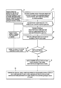
FIG. I illustrates a flowchart of a method of estimating model parameters in
accordance with
one or more embodiments of the invention.
FIGS. 2A and 2B illustrate methods for model parameterization, in accordance
with one or
more embodiments of the invention.
5b
CA 02749831 2016-08-17
FIG. 3A to 3E illustrate a conductivity model and the calculated model
parameter variances,
means, modes, and medians, according to one or more embodiments of the
invention.
5c
CA 02749831 2011-07-14
WO 2010/090825 PCT/US2010/021457
FIG. 4 illustrates a boundary-based multi-dimensional model of the subsurface,
according to
one or more embodiments of the invention.
FIG. 5 illustrates a system for performing stochastic inversion methods in
accordance with
one or more embodiments of the invention.
DETAILED DESCRIPTION
Embodiments of the invention provide a computer implemented stochastic
inversion method
for estimating model parameters of an earth model. In an embodiment, the
method utilizes a
sampling-based stochastic technique to determine the probability density
functions (PDF) of
the model parameters that define a boundary-based multi-dimensional model of
the
subsurface. In some embodiments a sampling technique known as Markov Chain
Monte
Carlo (MCMC) is utilized. MCMC techniques fall into the class of "importance
sampling"
techniques, in which the posterior probability distribution is sampled in
proportion to the
model's ability to fit or match the specified data set or sets. Importance
sampling results in
an uneven sampling of model space which characterizes the areas of high
probability with
reduced number of forward function calls compared to more traditional sampling
techniques.
In another embodiment, the inversion includes the joint inversion of multiple
geophysical
data sets. Embodiments of the invention also relate to a computer system
configured to
perform a method for estimating model parameters for accurate interpretation
of the earth's
subsurface.
Referring now to FIG. 1, this figure shows a method 10 for estimating model
parameters of
an earth model. The operations of method 10 presented below are intended to be
illustrative.
In some embodiments, method 10 may be accomplished with one or more additional
6
CA 02749831 2011-07-14
WO 2010/090825 PCT/US2010/021457
operations not described, and/or without one or more of the operations
discussed.
Additionally, the order in which the operations of method 10 are illustrated
in FIG. 1 and
described below is not intended to be limiting.
The method 10 starts at an operation 12, where at least one geophysical data
set is acquired.
Each geophysical data set samples some portion of a subsurface geological
volume of interest
and is used to define a geophysical acquisition geometry of the geological
volume of interest.
The geophysical data set may include, for example, controlled source
electromagnetic data
(CSEM), magnetotelluric data, gravity data, magnetic data, seismic data, well
production data
or any combination of the foregoing.
The geophysical acquisition geometry is the locations in space (X,Y,Z) of the
sources and
receivers as well as any system operating parameters such as source tow speed
and
parameters that fully describe the source wave-form as a temporal function.
At operation 14, a specified number of boundary-based multi-dimensional models
of the
subsurface geological volume of interest are generated. In an embodiment, each
model is
comprised of model parameters which are defined at a plurality of locations in
the geological
volume of interest called nodes. A specified number of boundary-based multi-
dimensional
models arc generated by taking the initial model parameters, as mean values
along with a user
defined model parameter variance to randomly select a new set of model
parameter values
from a user defined distribution (usually a Gaussian distribution, but other
distributions are
possible). Each set of unique model parameters define a two dimensional (2D),
3D or 4D
model of the geological volume of interest.
7
CA 02749831 2011-07-14
WO 2010/090825 PCT/US2010/021457
In another embodiment, each model parameter has values comprising an X, Y and
Z value for
defining the node location in space and at least one geophysical property
value. In an
embodiment, the geophysical property value can include electrical conductivity
or resistivity
(a), compressional velocity (Vp), shear velocity (Vs) and density(p). In
addition, the
geophysical property values can include reservoir parameters such as fluid
saturations,
pressure, temperature and/or porosity. These reservoir paramaters can be
included by
incorporating a rock physics model (derived from well log data), which link
the geophysical
parameters to the reservoir parameters. By way of non-limiting example, the
model can be
parameterized in terms of the geophysical properties as discussed above and/or
reservoir
properties, such as fluid saturation and porosity. In an embodiment, the
geophysical property
values are interpolated in space between a unique set of nodes to define the
model boundaries
and to generate the model parameters required for the calculation of the
forward model
responses. The boundary-based multi-dimensional models can then be projected
onto a finite-
difference or finite-element mesh for calculation of the forward model
responses. The
projection process is done such that cells which straddle a boundary are
assigned a property
value which is derived from a spatially weighted average of the property above
and below the
boundary.
Generalized representations of model parameterization, in accordance with one
or more
embodiments of the invention, are shown in FIG 2. FIG. 2A shows a standard
cell based
model parameterization. The geophysical property at each cell 32 is a model
parameter with
regularization or smoothing applied to all adjacent cells 34. The cell model
is typically used
in a finite-difference or finite-element calculation to generate the model
response. FIG 2B
shows boundary-based model parameterization. Nodes 36 controlling boundaries
38 can be
the model parameters, each node having a location and geophysical property
value(s). The
8
CA 02749831 2011-07-14
WO 2010/090825 PCT/US2010/021457
model parameters can be interpolated laterally and vertically between nodes.
In an
embodiment, the resulting boundary-based model can be projected onto a finite-
difference or
finite-element mesh for calculation of the forward model response.
Boundary-based model parameterization shown in FIG. 2B, solves several
inherent problems
with the traditional cell based model parameterization. As an illustration, a
typical 2D finite-
difference mesh would require on the order of 10 to 100 thousand cells to
accurately calculate
the forward model response to a model of interest. If the geophysical property
of each cell is
used as a model parameter in an inversion, there are two major problems
created for a
stochastic inverse. First, the conductivities of adjacent cells are highly
correlated, as shown
in FIG. 2A, causing convergence to be slow. Second, the cell based model
parameterization
does not correspond well to sedimentary geology with its inherent layered
structure, with
boundary between layers of relatively uniform properties. Boundary-
based model
parameterization greatly reduces the number of model parameters, only model
parameters at
nodes are used in the inversion, while at the same time the boundaries of the
model
correspond to geologic boundaries.
Referring back to FIG. 1, at operation 16, forward model responses of the
models for each
specified acquisition geometry are generated. The model comprised of all the
model
parameters at nodes on the boundaries is forward modeled by projecting the
geophysical
properties, such as conductivity, onto a finite-difference or finite element
mesh and
calculating the forward model response. At operation 18 numerical calculations
are used to
generate a likelihood value of the forward model responses matching the
geophysical data set
for each specified acquisition geometry. The inverse problem is defined as a
Bayesian
9
CA 02749831 2011-07-14
WO 2010/090825 PCT/US2010/021457
inference problem which requires defining the model likelihood function as
well as the prior
distribution of model parameters. In its simplest form this results in:
f (P I d) oc f (d P)f (P) (3)
Where f(pd) is the joint posterior PDF of all unknown model parameters, p
given the data d.
The first ten-n on the right side of the equation, f(d p), is the likelihood
function of data, d,
given model parameters p, and the last term on the right side, f(p), is the
prior distribution of
all unknown model parameters. The likelihood function, f(d p), can take
various forms
depending on the model used to describe the noise in the data. By way of non-
limiting
example, for electromagnetic data E, when the error is assigned as a
percentage of the
measurement, it takes the form:
(E o-) =nun exp e.fk
1=1 k=1 irg j2; 2 fij2 euk
(4)
where the model electrical conductivity is o-. The observed electric field, e,
is a function of
frequency (total number of frequencies equal to rd), offset, (total number of
offsets equal to
no), and is complex resulting in 2 components (real and quadrature). The
forward model
ill' (0-)
response is . The error fi , is a function of offset (j) and is a percent
of e.
If reflection seismic data is modeled in the shot domain where there are N,
time samples and
Na reflection angles the forward modeled seismic data can be represented as:
CA 02749831 2011-07-14
WO 2010/090825 PCT/US2010/021457
a
Ti] = (vp,vs, p) + Eij (5)
where i is the time index (1 to Nt) and j is the angle index (1 to Na), S is
the seismic forward
problem and t: is the measurement error. If the errors are assumed to be
Gaussian then the
seismic likelihood function, f, would be:
f (SVP,Vs,P) =v/(27)21Z1 exp (¨ -2 JE-1E) (6)
Where, e is the vector of data errors and E is the data covariance matrix.
In some embodiments, MCMC sampling techniques can be used to estimate f(4).
Traditional Monte Carlo methods are impractical due to the high number of
model
parameters and high dimensionality of the problems to solve. In conjunction
with the
MCMC approach to the stochastic inverse equations (4) and (6) the use of
boundary-based
model parameterization illustrated in FIG. 2B can also be utilized to reduce
the number of
model parameters in the equation.
In some embodiments, more than one data type and its associated acquisition
geometry may
be used. For example a non-limiting example would be the combination of CSEM
and
seismic reflection data. In this case the geophysical parameters at each
boundary node would
be electrical conductivity, compressional velocity, shear velocity and
density. The seismic
forward model, represented by S in equations (5) and (6) above could be a
finite-difference or
finite-element implementation of the elastic wave equation. When the error is
assumed to be
11
CA 02749831 2011-07-14
WO 2010/090825 PCT/US2010/021457
Gaussian the associated likelihood function for the seismic data would be of
the form of
equation (6) above.
If seismic data is added then the Bayesian inverse problem, equation (3), must
be modified
to:
fsE(Pid) f (sIvp, vs, p)f (E10-)f (vp, vs, p)f (a) , (7)
wherefsE is the combined pdf, f (SIVp , Vs, p) is the seismic likelihood
function (equ. 6),
f (E I o-) is the CSEM likelihood function (equ. 4), f (Vp, Vs , p) is the
prior for the seismic
parameters and [(o-) is the prior for the conductivity parameters.
At operation 20 illustrated in Fig. 1 the model parameters are saved as one
element of a
Markov Chain for each model. The number of Markov Chains is equivalent to the
number of
specified models at the beginning of the inversion. It should be appreciated
by one skilled in
the art that a number of MCMC sampling algorithms exist, for example, a
combination of
Metropolis-Hastings (Hasting, 1970) sampling and Slice Sampling (Neal, 2003)
can be used
to generate a sequence of model parameters that form Markov Chains.
Determination is made at operation 22 as to whether convergence of the Markov
Chains is
obtained within a defined tolerance. The Markov Chains are converged when the
PDFs of
the model parameters are an accurate representation of the true distributions,
given the level
of noise, so that the statistical moments of the distributions (mean, median,
mode and
variance) are accurate. Markov Chains can be run more than once, either
sequentially, or in
parallel in order to determine convergence. Many methods can be used to
determine
12
CA 02749831 2011-07-14
WO 2010/090825 PCT/US2010/021457
convergence of the Markov chains, such as the methods developed by Gelman and
Rubin
(1992) and Raftery and Lewis (1992). In one embodiment the method of Gelman
and Rubin
is used where the convergence test computes the within-sequence variance W and
the
between-sequence variance B/n as follows:
1
B I n = _________________________________________ (8)
m ¨1
1
W = in(n ¨1) Em. Et" (19 .t 1-1)2 (9)
1=1 =1 I -1
where 111 is the number of Markov Chains, n is the number of samples in the
chain, and pit is
the tth of the n iterations of p in chain j.
Having computed (8) and (9) an estimate of the model parameter variances ,
(72, is computed
by a weighted average of B and Was:
2 n ¨1 B
(10)
The potential scale reduction factor is computed as:
R= (11)
in W inn
13
CA 02749831 2011-07-14
WO 2010/090825 PCT/US2010/021457
If R, equation (11), is close to 1 the chains are considered to have
converged. The
determination of how close is "close enough" is done by testing on synthetic
models prior to
inversion of real data. For example, a value of 1.1 for R may be sufficient in
some
embodiments of the present invention.
At operation 24 the values of the model parameters for each model are updated.
If at
operation 22 convergence is not obtained (R is not close to 1) the model
parameters are
updated by any number of sampling algorithms. A non-limiting example would be
the use of
the Metropolis-Hastings sampling algorithm, using the existing parameter
values as mean
values and a Gaussian distribution of assumed variance to draw a new value for
each model
parameter. Another possibility is the use of the Slice-Sampling algorithm to
generate new
model parameters. In one embodiment, the choice of the sampling algorithm at
each iteration
is determined by a random draw of a uniform variable where the probability of
each sampling
technique being used on any iteration is assigned at the start of the
inversion. For example,
assign a probability of 0.4, 0.4, 0.1, 0.1 for multi-variant Metropolis-
Hasting, multi-variant
Slice-Sampling, uni-variant Metropolis-Hasting, and uni-variant Slice-Sampling
respectively,
then at each iteration a uniform random number is generated and its value
determines which
sampling technique is used. Once a new model is generated the workflow 10
proceeds to
operation 26 and operations 14 to 22 are repeated until convergence is reached
within a
defined tolerance, i.e. when the PDFs of the model parameters arc an accurate
representation
of true distributions in the model parameters. The Markov Chains may not
converge if there
are insufficient iterations or if there are an insufficient number of Markov
Chains. When R,
equation (11), is within a defined tolerance of the value 1, the Markov Chains
have
converged and sampling can stop. The algorithm is implemented both for serial
(single
processor) and parallel (clusters) computing. The serial implementation is for
simple model
14
CA 02749831 2011-07-14
WO 2010/090825 PCT/US2010/021457
testing and algorithm refinement while the parallel implementation is best
suited for large
scale production inversions.
If convergence is obtained at operation 22, the method proceeds to operation
28 where all the
model parameter values from the chains are binned to produce a PDF for each
parameter. The
PDF gives the probability that the model parameters are consistent with the
geophysical data
set. The PDF contains the most likely value of the model parameters and
quantifies the
uncertainty in the estimate.
At operation 30, the PDFs for each model parameter resulting from operation 28
are used to
calculate the variances, means, modes, and medians of each model parameter for
each model
of the subsurface geological volume of interest. Joint inversion of multiple
geophysical data
types, each sensitive to different physical properties of reservoir materials,
provide better
estimates of the earth model parameters than inversion of individual data
sets.
In an embodiment, the calculated mean, mode and median of each model parameter
PDF is
used as model parameter values and a forward simulation is performed to
compute a data root
means square (RMS) data misfit. This is a measure of how well the calculated
data fits the
geophysical data set. The user is presented with 3 models from the mean, mode
and median
of the model parameter PDFs and the associated RMS data misfit. In addition,
the variance
of each model parameter can be computed along with a graphical illustration of
the PDF and
the mean, mode and median values. Providing better estimates of model
parameters which
are used to interpret the subsurface geological volume of interest.
CA 02749831 2011-07-14
WO 2010/090825 PCT/US2010/021457
In another embodiment, the user can use any or all of these three models as
starting models
for a deterministic inversion (least squares), a minimization of equation (1),
to find the model
with the lowest RMS data misfit. This operation provides a deterministic
inverse with an
improved starting model which greatly increases its chances of reaching the
global minimum.
It will be appreciated that the workflow of FIG 1. is intended to encompass
several scenarios
for estimating model parameters. In some embodiments method 10, using boundary-
based
model parameterization coupled with a stochastic inversion, is extended to
include the joint
inversion of multiple data types to estimate a single self consistent model.
In other
embodiments the joint inversion models can be parameterized in terms of the
geophysical
and/or reservoir properties. The approach can be implemented in 2D, 3D and 4D.
In a non-
limiting example, the finite-element based inversion algorithm shown in
equation (4) is
implemented using stochastic MCMC sampling of a boundary-based model
parameterization.
The modelled geophysical property is the conductivity (a). In 2D the
boundaries are
described using linear interpolating functions between nodes on a CSEM towline
(the
horizontal axis) and depth on the vertical axis. In 3D the boundaries are
described by nodes
in X, Y and Z with a hi-linear or higher-order interpolating function used to
produce surface
Z and model conductivity values at arbitrary locations within the 3D model.
The electrical
conductivity can be a scalar, a vector or a tensor for isotropic, transverse
anisotropic or full
anisotropic models respectively. For the isotropic case, the value of a is
independent of the
coordinate direction. For transverse anisotropy there are 3 components (ax,
ay, az) of
conductivity, each of which can be independently estimated. The most general
case, full
anisotropy, results in a symmetric conductivity tensor given by,
16
CA 02749831 2011-07-14
WO 2010/090825 PCT/US2010/021457
avx axy axz
a(9)
yx 1E
azx fy azz
where the off-diagonal terms are symmetric, (axy = ayx, etc.). Hence, the
inversion for
isotropic, transverse anisotropic and full anisotropy results need to estimate
1, 3 or 6
conductivity parameters respectively per node per surface in the inversion. In
other
embodiments where other geophysical data are used, such as seismic, the
associated
geophysical parameters would be treated just as explained for electrical
conductivity.
Traditionally the use of 3D seismic data at successive times over a producing
reservoir to
image changes in the reservoir is referred to as 4D. The new inversion
technique can be used
as a 4D technique to monitor changes in the earth over time as production
occurs from a
petroleum reservoir by inverting observed data taken at progressive times
during productions.
Observed data at each time step is inverted and the changes between times are
used to
determine where the reservoir is changing.
FIG. 3 illustrates a conductivity model, according to one or more embodiments
of the
invention. A simple layered 1D conductivity model of P1 ¨ P4 is shown in FIG.
3A. The
simulated responses to a CSEM survey acquisition geometry are shown in FIGs 3B-
3E. FIG.
3B corresponds to P1, FIG. 3C corresponds to P2, FIG. 3D corresponds to P3,
FIG. 3E
corresponds to P4. The electromagnetic source is located 50m above the sea
floor with the
electromagnetic receivers placed on the sea floor. The source is an electric
dipole operated at
0.25, 0.75 and 1.25 Hz. The receivers are offset from the source from 500 to
1500 m. The
simulated data had 10 percent Gaussian random noise added prior to inversion.
17
CA 02749831 2011-07-14
WO 2010/090825 PCT/US2010/021457
While the gradient based algorithm given by equations (1) and (2) can find a
solution, in this
example, that is as close to the true values (True Value) as are the modes of
the PDF's (PDF
Mode), the resulting model parameter standard errors (Coy SD) are between a
factor of 2 and
too small. This is a critical short coming of a traditional inversion approach
if the resulting
model error estimates are to be used in any quantitative risk assessment
process. The model
parameter error calculation from the model covariance matrix at the minimum of
equation (1)
is insufficient compared to the model parameter PDF standard errors (PDF SD).
FIG. 4 illustrates a method of stochastic inversion, according to one or more
embodiments of
the invention. A graphical illustration 40 is shown of a 2D boundary-based
model having 10
layers. Nodes controlling boundary 42 depth (Z) are black filled diamonds 44,
nodes
controlling geophysical properties are open squares 46. White lines are
horizons 48
interpreted from seismic data. Grey scale is electrical conductivity, with
light being
conductive and dark being resistive. Example resistivity PDF's are shown for 2
nodes. The
model shown uses the mode of each PDF as the node conductivity.
In some embodiments, method 10 may be implemented in one or more processing
devices
(e.g., a digital processor, an analog processor, a digital circuit designed to
process
information, an analog circuit designed to process information, a state
machine, and/or other
mechanisms for electronically processing information). The one or more
processing devices
may include one or more devices executing some or all of the operations of
method 10 in
response to instructions stored electronically on an electronic storage
medium. The one or
more processing devices may include one or more devices configured through
hardware,
firmware, and/or software to be specifically designed for execution of one or
more of the
operations of method 10. A system configured to execute a computer readable
medium
containing a program which, when executed, performs operations of the method
10 is
18
CA 02749831 2016-08-17
,
schematically illustrated in Figure 5. A system 50 includes a data storage
device or memory
52. The stored data may be made available to a processor 54, such as a
programmable general
purpose computer. The processor 54 may include interface components such as a
display 56
and a graphical user interface 58. The graphical user interface (GUI) may be
used both to
display data and processed data products and to allow the user to select among
options for
implementing aspects of the method. Data may be transferred to the system 50
via a bus 60
either directly from a data acquisition device, or from an intermediate
storage or processing
facility (not shown).
Although the invention has been described in detail for the purpose of
illustration based on
what is currently considered to be the most practical and preferred
embodiments, it is to be
understood that such detail is solely for that purpose and that the invention
is not limited to the
disclosed embodiments, but, on the contrary, is intended to cover
modifications and equivalent
arrangements that are within the scope of the appended claims. For example, it
is to be
understood that the present invention contemplates that, to the extent
possible, one or more
features of any embodiment can be combined with one or more features of any
other
embodiment.
19