Note: Descriptions are shown in the official language in which they were submitted.
CA 02750093 2011-08-18
GAL235-1CA
1
Method for Computing and Storing Voronoi Diagrams, and Uses Therefor
FIELD AND BACKGROUND OF THE INVENTION
The present invention relates to a method for computing and storing Voronoi
diagrams
and to uses thereof in technology and, more particularly, but not exclusively
to uses thereof in
communications networks, in robotics, in three-dimensional networks, in
materials science, in
molecular biology, in searching of data, in a way of providing overall control
of a variety of
methods for applications such as image processing, data categorization,
numerical simulations,
meshing, solid modelling, clustering etc, efficient designs of electronic
circuits, for
management of geographical information systems, efficient location problems,
face
recognition and image recognition in general, as an artistic tool, and as a
programming tool.
Voronoi diagrams are one of the basic structures in computational geometry.
Roughly
speaking, they are a certain decomposition of a given space into cells,
induced by a distance
function and by a tuple of subsets, called the generators or the sites. More
precisely, given a
collection of sites, a Voronoi cell corresponding to some site Pk is the set
of all the points
whose distance to Pk is not greater than their distance to the union of the
other sites Pi P.
Voronoi diagrams appear in a large number of fields in science and technology
and
have many applications. One can find applications in chemistry, biology,
archeology,
mathematics, physics, computer graphics, image processing, computational
geometry,
crystallography, geography, metallography, economics, art, computer science,
astronomy,
linguistics, robotics, communication and many more areas. A very simple
example which
illustrates the concept of a Voronoi diagram is a collection of competing
shops in a two-
dimensional city. Each shop is represented by a point, and the Voronoi cell
associated with it
is its domain of influence: the region composed of all the points whose
distance to this specific
shop is not greater than their distance to the other shops. An illustration is
given in Figures 1
and 2. As a result of the above, it can be seen that finding methods for
computing Voronoi
diagrams is an important task.
There are many methods for computing Voronoi diagrams, but they suffer from
several
limitations. They suffer from degenerate cases and their implementation is
complicated in
many cases. Their computation time can grow significantly when the number of
sites grows.
Most of them are limited to the computation of diagrams of point sites, and
cannot compute
CA 02750093 2011-08-18
GAL235-1CA
2
diagrams whose sites consist of many points. In addition, most of them are not
able to
compute a specific cell independently of the other cells, and this obviously
imposes serious
limitation on the possibility of parallel implementation .
Some time ago the present inventor developed a general method for computing
Voronoi diagrams, this being disclosed in US Patent Application No.
12/461,216.
SUMMARY OF THE INVENTION
The present embodiments improve significantly upon the general method related
to
above, in the particular but important case of the Euclidean distance. In
addition, the present
embodiments allow for retrieving and storing in a convenient way the
combinatorial
information relating to the diagram, which was problematic in the previous
method.
According to one aspect of the present invention there is provided a
computerized
method of decomposing a given region X into cells, the decomposition being
induced by a set
of sites P1,..., Pn, and a distance function d, and finding for each desired
site Pk a cell, the cell
comprising a set of all the points in X satisfying a distance inequality
condition, based on said
distance function, the inequality of the condition being that the distance of
a respective point
to said site Pk is not greater than the distance of said respective point to
the union of the other
sites, the method being carried out on an electronic processor and comprising:
a) selecting a desired site Pk and a desired point p in this site;
b) selecting a plurality of subfaces corresponding to a manifold around said
point p;
c) for each desired subface selecting a plurality of directions;
d) for each direction providing a ray, selecting a point on the ray as an
endpoint, and
selecting hyperplanes corresponding to the endpoints;
e) for each desired subface determining a type of intersection between the
detected
hyperplanes;
f) determining whether there exist vertices of the cell in a cone generated by
the
endpoints, and finding said vertices, wherein if there remain further vertices
that have not been
found then there is carried out a step of further dividing the said subface
into additional
subfaces for separate determination;
g) storing information relating to said vertices;
CA 02750093 2011-08-18
GAL235-1CA
3
h) repeating a) - g) for each desired site Pk and each desired point p in the
selected
site;
i) defining at least one vertex or hyperplane from said endpoints, thereby
decomposing
said region X; and
j) outputting said decomposed region X in a machine readable format.
The method may further comprise providing the decomposed region for use in any
of
the following: controlling a communications network, managing a communication
network,
controlling a robot, managing a robot, modeling, testing or simulating a three-
dimensional
network, controlling a three-dimensional network, testing or modeling a
material, data
searching, searching for data on a network or database, image processing, mesh
generation and
re-meshing, curve and surface generation, curve and surface reconstruction,
solid modeling,
collision detection, controlling motion of vehicles, navigation, accident
prevention, data
clustering and data processing, proximity operations, nearest neighbor search,
numerical
simulations, weather prediction, analyzing or modeling proteins, analyzing or
modeling crystal
growth, analyzing or processing digital or analog signals, analyzing or
modeling biological
structures, designing drugs, finding shortest paths, pattern recognition,
rendering, data
compression, providing overall control of a plurality of methods for image
processing,
providing overall control of a plurality of methods for data categorization,
providing overall
control for a plurality of methods for data clustering, designing and testing
of electronic
circuits, management of geographic information systems, computing geometric
objects,
locating a resource according to the solution of an efficient location
problem, face recognition,
analyzing the behavior of populations, analyzing or modeling data related to
astronomy,
analyzing or modeling data related to geography, detecting or analyzing
geometric structures,
detecting or analyzing space structures, location based services, analyzing
traffic, analyzing
atmospheric data, analyzing oceanographic data, detecting or analyzing the
distribution of
matter in a region, detecting or analyzing the distribution of populations in
a region, detecting
or analyzing the distribution of energy in a region, and an artistic tool .
The method may involve, in step d), additionally selecting neighbour sites
that
correspond to said hyperplanes.
In an embodiment, said determining said type comprises examining a
predetermined
system of equations.
CA 02750093 2011-08-18
GAL235-ICA
4
In an embodiment, said determining of vertices in said cone comprises further
examining said predetermined system of equations.
In an embodiment, said manifold is a simplex.
In an embodiment, a subface to be selected is determined by one member of the
group
consisting of corners and unit vectors corresponding to said corners.
In an embodiment,said predetermined system of equations is of the general form
B?. =H,
wherein:
m is the dimension of said region X;
O , i=l,...,m are said direction unit vectors;
p +Ti is said endpoint in direction 0i;
Ti T(0i,p)0i is the vector whose direction is Oi and whose length is the
distance between said
point p and said endpoint p+T_i;
L i is the hyperplane corresponding to the endpoint p +Ti;
Ni is a normal to the hyperplane Li;
X (X1,= =,gym) is a vector of unknowns;
B is an m by m matrix with Bij=<Ni,TT >, ij= 1,2,...,m; and
H=(H1,...,Hm) is the vector with Hi= <Ni,Ti >, i=1,2,...,m.
In using the term "of the form", it is intended to include all non-material
transformations and
variations of the formula that do not effect the way it works, including
multiplication by a
scalar.
The method may comprise:
computing respective vertices by solving said predetermined system of
equations to
obtain a solution ),=(X1,..., , and
checking if a corresponding vector u=p-l 1T1+...? Tm, comprising said vectors
T1,...,Tm and said point p, is in said cone and in said cell. wherein m is the
dimension of said
region X.
CA 02750093 2011-08-18
GAL235-1CA
In an embodiment, said region X is of dimension two, wherein said dividing
said given
subface into additional subfaces comprises choosing an intermediate vector
between
respective corners of said subface to create two new subfaces, each new
subface comprising
said intermediate point and one of said corners, or vectors in a direction of
said corners.
5 In an embodiment, said region X is of dimension two and wherein said
deciding
whether there are vertices of the cell in said cone generated by said
endpoints comprises
checking one member of the group consisting of:
a number of said hyperplanes,
whether there exist nonnegative solutions to said system of equations,
whether the determinant of said matrix B vanishes or not,
whether there are infinitely many solutions, a unique solution or no solution
at all to
said system of equations.
In an embodiment, said region X is of dimension three and said dividing said
given
subface into additional subfaces comprises dividing said subface into a
partition of additional
subfaces, where said partition is chosen from the following list of possible
partitions:
no partition at all,
a small diameter partition',
an interior point partition of type 0,
an interior point partition of type 1,
an interior point partition of type 2,
an interior point partition of type 3,
a boundary point partition of type 1,
a boundary point partition of type 2, and
a boundary point partition of type 3.
In an embodiment, said region X is of dimension three and said deciding
whether there
are vertices of the cell in said cone generated by said endpoints comprises
one member of the
group consisting of:
checking the number of different hyperplanes,
checking whether there exist nonnegative solutions to said system of
equations,
checking whether said matrix B is of rank 1, or rank 2, or rank 3, or of rank
smaller
than the rank of another matrix BH, or
CA 02750093 2011-08-18
GAL235-1CA
6
checking whether there are infinitely many solutions, unique solution or no
solution at
all to said system of equations.
In an embodiment, the computations are carried out to a predetermined level of
error
parameters.
An embodiment may reuse cell calculations of earlier stages for saving
calculations in
later stages .
In an embodiment, said computation of a respective endpoint in a given
direction 0
comprises:
selecting a point y along the corresponding ray in direction 0, and moving and
testing y
recursively, and until a stopping condition is satisfied:
recursively testing comprises: selecting a point y along the ray emanating
from p and
in cases of y being either on the boundary of said region X or outside the
cell of p; then if y is
on the boundary, defining L as a corresponding hyperplane on which y is
located and checking
whether y is in said cell; and if y is in said cell, selecting y as an
endpoint and defining L as
the corresponding bisecting hyperplane on which y is located; and
wherein if y is neither within said cell of p nor on a boundary of region X,
finding a
corresponding point closer to y than to p, and determining an intersection u
between the ray
and a corresponding hyperplane L then setting y: =u, recursively testing until
y is in said cell of
p then setting y as the endpoint, said corresponding point being a closest
neighbor site or a
point in said closest neighbor site, and L being the corresponding bisecting
hyperplane.
According to a second aspect of the present invention there is provided a
computerized
method for storing computed Voronoi cells and retrieving combinatorial
information related to
said cells to an electronic storage device, the method comprising:
storing, in said storage device, for each desired site Pk and each desired
point p, data
relating to a desired vertex u belonging to the cell of said point p together
with data relating to
an associated hyperplane; and
using said information to obtain information about said cells.
In an embodiment, said associated hyperplane is a hyperplane on which is
located a
face belonging to the cell of said point p.
In an embodiment, said data relating to desired vertex comprises the
coordinates of
said desired vertex and said data relating to said associated hyperplane
comprises at least one
CA 02750093 2011-08-18
GAL235-1CA
7
member of the group comprising: associated neighbor sites, associated
bisecting hyperplanes,
associated faces located on said hyperplanes, and endpoints,
The method may comprise applying said combinatorial information to one member
of
the group comprising: controlling a communications network, managing a
communication
network, controlling a robot, managing a robot, modeling, testing or
simulating a three-
dimensional network, controlling a three-dimensional network, testing or
modeling a material,
data searching, searching for data on a network or database, image processing,
mesh
generation and re-meshing, curve and surface generation, curve and surface
reconstruction,
solid modeling, collision detection, controling motion of vehicles,
navigation, accident
prevention, data clustering and data processing, proximity operations, nearest
neighbor search,
numerical simulations, weather prediction, analyzing or modeling proteins,
analyzing or
modeling crystal growth, analyzing or processing digital or analog signals,
analyzing or
modeling biological structures, designing drugs, finding shortest paths,
pattern recognition,
rendering, data compression, providing overall control of a plurality of
methods for image
processing, providing overall control of a plurality of methods for data
categorization,
providing overall control for a plurality of methods for data clustering,
designing and testing
of electronic circuits, management of geographic information systems,
computing geometric
objects, locating a resource according to the solution of an efficient
location problem, face
recognition, analyzing the behavior of populations, analyzing or modeling data
related to
astronomy, analyzing or modeling data related to geography, detecting or
analyzing geometric
structures, detecting or analyzing space structures, location based services,
analyzing
atmospheric data, analyzing oceanographic data, detecting or analyzing the
distribution of
matter in a region, detecting or analyzing the distribution of populations in
a region, detecting
or analyzing the distribution of energy in a region, and an artistic tool .
The method may comprise finding, from said stored data, different neighbors of
each
site p; computing therefrom a Delaunay tessellation; and passing an edge
between each site p
and each of its different neighbor sites.
Unless otherwise defined, all technical and scientific terms used herein have
the same
meaning as commonly understood by one of ordinary skill in the art to which
this invention
belongs. The materials, methods, and examples provided herein are illustrative
only and not
intended to be limiting.
CA 02750093 2011-08-18
GAL235-1CA
8
The word "exemplary" is used herein to mean "serving as an example, instance
or
illustration". Any embodiment described as "exemplary" is not necessarily to
be construed as
preferred or advantageous over other embodiments and/or to exclude the
incorporation of
features from other embodiments.
The word "optionally" is used herein to mean "is provided in some embodiments
and
not provided in other embodiments". Any particular embodiment of the invention
may include
a plurality of "optional" features unless such features conflict.
Implementation of the method and/or system of embodiments of the invention can
involve performing or completing selected tasks manually, automatically, or a
combination
thereof.
Moreover, according to actual instrumentation and equipment of embodiments of
the
method and/or system of the invention, several selected tasks could be
implemented by
hardware, by software or by firmware or by a combination thereof using an
operating system.
For example, hardware for performing selected tasks according to embodiments
of the
invention could be implemented as a chip or a circuit. As software, selected
tasks according to
embodiments of the invention could be implemented as a plurality of software
instructions
being executed by a computer using any suitable operating system. In an
exemplary
embodiment of the invention, one or more tasks according to exemplary
embodiments of
method and/or system as described herein are performed by a data processor,
such as a
computing platform for executing a plurality of instructions. Optionally, the
data processor
includes a volatile memory for storing instructions and/or data and/or a non-
volatile storage,
for example, a magnetic hard-disk and/or removable media, for storing
instructions and/or
data. Optionally, a network connection is provided as well. A display and/or a
user input
device such as a keyboard or mouse are optionally provided as well.
BRIEF DESCRIPTION OF THE DRAWINGS
The invention is herein described, by way of example only, with reference to
the
accompanying drawings. With specific reference now to the drawings in detail,
it is stressed
that the particulars shown are by way of example and for purposes of
illustrative discussion of
the preferred embodiments of the present invention only, and are presented in
order to provide
what is believed to be the most useful and readily understood description of
the principles and
conceptual aspects of the invention. In this regard, no attempt is made to
show structural
CA 02750093 2011-08-18
GAL235-1CA
9
details of the invention in more detail than is necessary for a fundamental
understanding of the
invention, the description taken with the drawings making apparent to those
skilled in the art
how the several forms of the invention may be embodied in practice.
In the drawings:
Figure 1 is a prior art illustration of the concept of a Voronoi diagram used
for
determining the domain of influences of twenty shops in a two-dimensional
city. Each shop is
represented by a point, and its domain of influence is represented by a cell
which is a polygon;
Figure 2 shows the boundaries of the cells of Figure 1;
Figure 3A shows an example of a Voronoi diagram of sites which are not points;
Figure 3B is a simplified flow chart that illustrates a method of generating a
Voronoi
diagram such as that shown in Fig. 1, by subdividing a region, according to a
first embodiment
of the present invention;
Figure 3C illustrates in greater detail the overall method of Fig. 3B;
Fig. 3D is a simplified flow chart illustrating the computing of endpoints for
the
method of Fig. 3C;
Fig. 3E is a simplified flow chart illustrating a routine for storing data
generated by the
method of Figs 3B or 3C or 3D;
Fig. 3F illustrates a method of generating the Delauney graph using the
information
stored in accordance with the method of Fig. 3E;
Figure 4 shows an example of several 3-dimensional Voronoi cells of point
sites,
together with some of the sites, bounded within a large overall box;
Figure 5 shows a more complicated 3-dimensional Voronoi cell;
Figure 6 shows the same cell of Figure 5 but from a different perspective;
Figure 7 shows an example of a 2-dimensional simplex (a triangle);
Figure 8 shows an example of a 3-dimensional simplex (a pyramid);
Figure 9 shows an illustration of the method of Fig. 3B for computing the
Voronoi
cells in the 2-dimensional case;
Figure 10 shows an illustration of the method of Fig. 3B for computing
endpoints;
Figure 11 shows a small diameter partition of a subface of a 3D simplex and
its sub-
faces, for the method of Fig. 3B for computing the Voronoi cells in the 3-
dimensional case;
Figure 12 shows an example of a boundary point partition of type 1 of a
subface of a
3D simplex and its sub-faces for the method of Fig. 3B in the 3-dimensional
case;
CA 02750093 2011-08-18
GAL235-1CA
Figure 13 shows an example of a boundary point partition of type 2 of a
subface of a
3D simplex and its sub-faces for the method of Fig. 3B in the 3-dimensional
case;
Figure 14 shows an example of a boundary point partition of type 3 of a
subface of a
3D simplex and its sub-faces for the method of Fig. 3B in the 3-dimensional
case;
5 Figure 15 shows an example of an interior point partition of type 0 of a
subface of a 3D
simplex and its sub-faces for the method of Fig. 3B in the 3-dimensional case;
Figure 16 shows an example of an interior point partition of type 1 of a
subface of a 3D
simplex and its sub-faces for the method of Fig. 3B in the 3-dimensional case;
Figure 17 shows an example of an interior point partition of type 2 of a
subface of a 3D
10 simplex and its sub-faces for the method of Fig. 3B in the 3-dimensional
case;
Figure 18 shows an example of an interior point partition of type 3 of a
subface of a 3D
simplex and its sub-faces for the method of Fig. 3B in the 3-dimensional case;
and
Figure 19 shows an example of a 2-dimensional Delaunay graph (Delaunay
tessellation) together with its associated Voronoi diagram.
DESCRIPTION OF THE PREFERRED EMBODIMENTS
The present embodiments comprise a method for computing with improved
efficiency
and storing 2-dimensional and 3-dimensional Euclidean Voronoi diagrams, and
applications
therefor. It allows the computation of each cell independently of other cells,
and hence
supports parallel implementation. The present embodiments meet the challenges
of degenerate
cases, and allow the computation of sites consisting of many points. The
present embodiments
further permit retrieval, in any dimension, of the combinatorial information
relating to the
diagram, such as the vertices, edges, faces, the neighbors of a given vertex,
and so on, and
storing such information in a simple and convenient manner. In particular, the
present
embodiments allow for the computation of a related structure called the
Delaunay graph (or
the Delaunay tessellation or the Delaunay triangulation) in a more efficient
way. The present
embodiments further provide a more efficient method for the exact computation
of endpoints.
The method disclosed in above mentioned US Patent Application No. 12/461,216
to
the present inventor, allows the approximate computation of general Voronoi
diagrams
(general distance functions, any dimension, etc.). The present embodiments
provide an
improvement thereon in the special but important case of the Euclidean
distance and
dimensions 2 and 3. The present embodiments further allow for retrieval and
storage in a
CA 02750093 2011-08-18
GAL235-1CA
11
convenient way of the combinatorial information relating to the diagram in any
dimension.
The calculation of the present embodiment may also be implemented in a manner
which is
orders of magnitude faster as compared with the previous method and may
provide more
precise results. The storage is also more efficient.
The following is an illustration of possible applications which can be
provided using
the present embodiments in particular, and which relate to Voronoi diagrams in
general.
There are several properties of the structure referred to as the Voronoi
diagram which
make it useful. Some of these properties are:
1. A Voronoi diagram induces a partition of a given space into cells, and it
is easier to
understand or analyze the cells, perform operations on them, etc, rather than
try to
apply an analysis on the whole space in one go. Furthermore, in many cases the
partition follows naturally from the given setting.
2. Sometimes useful information about the whole space or parts of the space
can be
obtained from certain other parts of the space, e.g., Voronoi generators or
the
boundaries of the Voronoi cells.
3. By the very basic definition of the Voronoi diagram, its cells are defined
by an optimal
property. Specifically, the cell of the site (generator) Pk is the set of all
the points in the
space whose distance Pk is not greater than their distance to the other sites.
Many
applications are designed for achieving an optimal solution to a given problem
and use
the above optimal property of the cells.
4. A Voronoi diagram is a geometric structure which is related to other
geometric
structures which are useful in themselves, such as the Delaunay graph (the
Delaunay
tessellation) or the convex hull. The relationship may be that the other
structures are
more easily computed from the Voronoi diagram, or more generally that the
Voronoi
diagram enables computing of these other structures.
5. Voronoi diagrams appear naturally in many places in science and technology.
CA 02750093 2011-08-18
GAL235-1CA
12
The following (far from being exhaustive) list of applications of Voronoi
diagrams follows
naturally from the properties discussed above.
1. Mesh generation and re-meshing, or rendering: the mesh is based on a
triangulation,
and the triangulation can be created directly by Voronoi diagrams or
indirectly using
Delaunay triangulation which is easily created by use of Voronoi diagrams.
2. Curve and surface generation/reconstruction, including solid modeling:
again, based
on triangulation, which approximates the surface. The triangulation may be
created
directly by using Voronoi diagrams or indirectly using Delaunay triangulation
which
is easily created from the Voronoi diagrams.
3. Robot motion in an environment with obstacles, collision detection: the
goal of the
robot is to move in a safe way, i.e.., to avoid colliding with the obstacles.
One
generates the Voronoi diagram of the obstacles (as generators), and the robot
moves
on the boundaries of the cells. The boundaries are those places in the space
which are
as far as possible from the obstacles. This is also good for any machine or
part thereof
which is not necessarily a robot, say a mechanical arm, but which moves in an
environment with obstacle, and subsequent references to robots herein are
intended to
refer to such machines or machine parts.
4. Motion of vehicles and/or accident prevention: The same principle applies
as with the
robot motion. The Voronoi diagram is computed and recomputed where the other
vehicles are moving generators. The cells allow each vehicle to find a safest
path. So
the Voronoi generators are the vehicles and the other obstacles in the
environment.
The solution is good for any kind of vehicles and moving vessels, including
land
vehicles, ships, and other seagoing vessels including submarines, aircraft,
satellites
and so on, and the term vehicle used herein is to be understood accordingly.
5. Clustering and data processing: the method is used for storing and
manipulating the
data in an efficient and convenient way. A data record may be provided as a
point in a
space, with several components (e.g., representing the longitude and latitude
of a
point, the age, salary and id number of a worker and so on), and one divides
the space
CA 02750093 2011-08-18
GAL235-1CA
13
using the Voronoi cells of certain points. Now one can efficiently and
conveniently
carry out operations on the data, for example because it is in a more simple
and
concise form. Operations that become easier include compression, searching,
further
subdividing and so on.
6. Proximity operations, nearest neighbor searches, data searches including
searching in
data bases, search engines, searching in files and so on. As in the previous
application
one partitions the space into the Voronoi cells of certain generators. Then,
starting
with an arbitrary initial point in the space, in order to find the generator
which is
closest or "resembles" this point, one only needs to determine the Voronoi
cell in
which the initial point is located.
7. Image processing: again, in order to analyze the image, a common way is via
partitioning the image into small parts and working with these parts. The
partitioning
may be carried out directly using a Voronoi diagram, or indirectly using the
Delaunay
tessellation.
8. Simulations, analyzing, modeling and prediction of phenomena which are
related to
Geographic Information System (GIS): these are dynamic phenomena which consist
of
a large amount of data which often changes rapidly. Again, one partitions the
space
using the Voronoi cells of certain generators (depending on the phenomenon) or
the
Delaunay tessellations, and the diagram/tessellation is updated according to
the
changes related to the phenomenon. One obtains a convenient data structure
which
allows one to do efficient and convenient operations on it. In particular,
this may help
in weather prediction; navigation; prediction of spreading of diseases,
contamination
and fires; helping designing better vehicles by better understanding the water
or air
flows around them and the like.
9. Numerical simulations including finite element methods: The procedure is as
with 8
above, but may be applied to many other phenomenon, including simulations of
astronomical phenomena, simulations of the behaviour of particles in a
solution,
motion/flow of vehicles in a highway or a crowd in a building, and so on.
CA 02750093 2011-08-18
GAL235-1CA
14
10. Tool for solving facility location: for instance, where to optimally
locate a new cellular
antenna, a new restaurant or a new school. The Voronoi diagram is created
using the
antennas, restaurants, etc. as the generators.
11. Molecular biology: analyzing and modeling proteins and other biological
structures.
Here the Voronoi generators are certain molecules or atoms. Additionally, the
Delaunay tessellation and other geometrical structures constructed from
Voronoi
diagrams (such as alpha and beta shapes) may be used. The application may help
in
understanding biological phenomena and designing drugs.
12. Material engineering: designing new materials or compounds. Analyzing and
understanding existing materials is carried out by partitioning the material
into the
Voronoi cells, where the generators may be certain atoms, molecules or even
defects
in the material and so on .
13. Designing and testing integrated circuits: Here one may use Voronoi
diagrams for
measuring and modeling what is called the critical area of an integrated
circuit. The
Voronoi diagram partitions the integrated circuit into Voronoi cells within
which
defects that occur cause electrical faults between the same two shape edges in
the
design. For computing the critical area for a particular fault mechanism, one
constructs
the Voronoi diagram for that particular fault mechanism.
14. Shortest paths: In one application one can use Voronoi diagrams for
finding the
shortest path between two points/shapes in a graph or an environment with
obstacles.
The shapes represent the generators and the boundaries of the Voronoi cells,
which are
used for computing the path. Examples include designing a better integrated
circuit by
saving the amount of wiring needed, or designing a better route for a bus or a
mechanical arm.
15. A tool for constructing useful geometric structures: For example the
Voronoi diagram
may be used to construct the Delaunay graph, otherwise known as the Delaunay
CA 02750093 2011-08-18
GAL235-1CA
tessellation, or the convex hull, or the medial axis, or a special case of
Voronoi
diagrams called centroidal Voronoi diagrams in which the sites are in the
center of
mass of their corresponding cells. These geometric structures in turn have
many
applications; for instance, Delaunay graphs and centroidal Voronoi diagrams
can be
5 used for image and signal processing, mesh generation, clustering, numerical
simulations and various others applications.
16. Pattern recognition, and computer graphics: The partition of the image
into Voronoi
cells of certain generators helps in analyzing the image and finding patterns
or key
10 features in the image. Another possibility is to construct the medial axis
or Delaunay
tessellation associated with a certain Voronoi diagram, and use the
construction for
pattern recognition. Examples include character recognition (OCR), and facial
recognition. Yet another possibility is to create an image having good
properties using
Voronoi diagrams.
17. Analyzing and designing communication networks: here the sites are the
static or
dynamic communication devices, for example antennas, cell phones, computers,
etc.
18. Signal processing and creating, coding: here the sites can be an element
in a video
signal, a digital code in a noisy environment and so on.
19. A tool for analyzing the behaviour and growth of crystals: the sites are
the points from
where the crystals start to grow.
20. Location based services: these are services based on geographic data and
may be
related to dynamic phenomena. The sites may be people, populations, cell
phones,
antennas, vehicles, shopping centres and so on. The service may be population
monitoring, analyzing the behaviour of customers, or consumers in general,
analyzing
traffic data, offering deals to costumers which are in the vicinity of a
business, etc.
CA 02750093 2011-08-18
GAL235-1CA
16
In the description below the following notation is used: one starts with a
region X,
called the world, and a collection of sets P1,P2,..., Pn called the sites or
the generators. The
dimension of the world X is denoted by m, usually 2 or 3, but in principle it
can be higher. The
elements in the world X are called points or vectors. A vector x in X has m
components and is
denoted by x=(x_l,...,x_m) or x=(x1,...xm). The length or norm of a vector
x=xl,...,xm) is
~ k=(~1J^2+...+Ixm r'2)"0.5 , i.e., the square root of the sum of the squares
of its elements. The
distance between any two points x=(x1,...,xm) and y=(Y1,...,ym) in the world
is measured
using a distance function d which is the Euclidean distance d(x,y)=((~1-
Y1j^2+...+ Jxm-
Ymr2)^0.5, i.e., the length of the vector x-y=(xl-Y1.... xm-Ym). The distance
between the
points x and y is also denoted by ~-y . The distance between a point x and a
set A is
d(x,A)=min{d(x,a): a in A}. The inner (scalar) product between the vectors
x=(xl,...,xm) and
Y(Y1,===,Ym) is 4c,y>=-X1=Y1+...+xm'Ym=
A vector x(xl,...,xm) is called nonnegative if the inequality xi>0 holds for
each
The dominance region (or domain of influence) of the set P with respect to the
set A is
the set of all the points in the world whose distance to the set P is not
greater than their
distance to the set A. It is denoted by dom(P,A).
Given the sites P1,...,Pn, the Voronoi cell of the site Pk is simply the set
of all the
points in the world whose distance to the site Pk is not greater than their
distance to the union
of the other sites Pj. In other words, it is the set dom(Pk, Ak) where Ak is
the union of all Pj, j
tk. Given a direction, represented by a unit vector 0 (i.e., 10 1=4), and
given some point p in
some site Pk, the point p+T(0,p)0 is the point of intersection of the ray
emanating from p in
direction 0 and the boundary of the cell of p. It is called the endpoint in
direction of 0. The
number T(0,p) is the distance from p to this endpoint .
A hyperplane is a line in dimension m=2, a plane in dimension m3 and so on.
Figure 4 shows an example of several 3-dimensional Voronoi cells of point
sites,
together with some of the sites, bounded within a large overall box.
CA 02750093 2011-08-18
GAL235-1CA
17
Figure 5 shows a more complicated 3-dimensional Voronoi cell.
Figure 6 shows the same cell of Figure 5 but from a different perspective.
A simplex is a triangle in dimension m=2, as illustrated in Figure 7 and is a
pyramid in
dimension m as shown in Fig. 8. A bisecting plane (or hyperplane)
corresponding to some
point u is a plane L which is in the middle between u and one of its neighbor
sites a (the plane
L passes via the middle of the interval [u,a] and is vertical to it). If u is
on the boundary of the
world X, i.e., on one of the world faces, the plane on which this face is
located will also be
called a bisecting plane of u. A bisector is a bisecting (hyper)plane.
The principles and operation of an apparatus and method according to the
present
invention may be better understood with reference to the drawings and
accompanying
description.
Before explaining at least one embodiment of the invention in detail, it is to
be
understood that the invention is not limited in its application to the details
of construction and
the arrangement of the components set forth in the following description or
illustrated in the
drawings. The invention is capable of other embodiments or of being practiced
or carried out
in various ways. Also, it is to be understood that the phraseology and
terminology employed
herein is for the purpose of description and should not be regarded as
limiting.
Reference is now made to Fig. 3B which illustrates a computerized method of
decomposing a given region X into cells. The decomposition is induced by a set
of sites P1,...,
Pn, and a distance function d, and involves finding for each desired site Pk a
cell. The cell that
is found is the cell that comprises a set of all the points in X satisfying a
distance inequality
condition, based on a distance function. The distance condition is that the
distance of a
respective point to the site Pk is not greater than the distance of the
respective point to the
union of the other sites, and such a decomposition is a way of defining the
generation of the
Voronoi diagram.
The method is suitable for carrying out on an electronic processor and may
comprise:
a) selecting a desired site Pk and a desired point p in the site;
b) selecting a plurality of subfaces corresponding to a manifold around the
point p;
c) for each desired subface selecting multiple directions;
CA 02750093 2011-08-18
GAL235-1CA
18
d) for each direction providing a ray, and selecting a point on the ray as an
endpoint,
then selecting hyperplanes corresponding to the endpoints;
e) for each desired subface determining a type of intersection between the
detected
hyperplanes;
f) determining whether there can be vertices of the cell in a non-negative
cone
generated by the endpoints, and finding these vertices. If there might remain
further vertices
that have not been found then there is carried out a step of further dividing
the subface into
additional subfaces for separate determination but stopping if a given stop
condition is
reached;
g) storing the vertices, hyperplanes, neighbor sites, and possibly endpoints,
in a
machine readable format, these being data relating to a vertex or hyperplane;
h) repeating a) - g) for each desired site Pk and each desired point p in the
selected
site;
i) defining at least one vertex or hyperplane from the endpoints, thereby
decomposing
the region X into subregions; and
j) outputting the decomposed region X in a machine readable format.
The Voronoi diagram generated by the above method may applied to uses
including
any of the following: controlling or managing a communications network,
controlling or
managing a robot, modeling, testing controlling or simulating a three-
dimensional network,
testing or modeling a material, data searching, searching for data on a
network or database,
image processing, mesh generation and re-meshing, curve and surface
generation, curve and
surface reconstruction, solid modeling, collision detection, controlling
motion of vehicles,
navigation, accident prevention, data clustering and data processing,
proximity operations,
nearest neighbor search, numerical simulations, weather prediction, analyzing
or modeling
proteins, analyzing or modeling crystal growth, analyzing or processing
digital or analog
signals, analyzing or modeling biological structures, designing drugs, finding
shortest paths,
pattern recognition, rendering, data compression, providing overall control of
a different
methods for image processing, providing overall control of different methods
for data
categorization, providing overall control of different methods for data
clustering, designing
and testing of electronic circuits, management of geographic information
systems, locating a
resource according to the solution of an efficient location problem, face
recognition, analyzing
CA 02750093 2011-08-18
GAL235-1CA
19
the behavior of populations, analyzing or modeling data related to astronomy,
analyzing or
modeling data related to geography, detecting or analyzing geometric
structures, detecting or
analyzing space structures, location based services, analyzing atmospheric
data, analyzing
oceanographic data, analyzing traffic, detecting or analyzing the distribution
of matter in a
region, detecting or analyzing the distribution of populations in a region,
detecting or
analyzing the distribution of energy in a region, and in providing an artistic
tool .
In stage d) it is possible additionally to select hyperplanes that correspond
to neighbor
sites or to the boundary of the region X.
The determination of a type of intersection may comprise a given system of
equations
under the conditions set by the vertex being examined, as will be discussed in
greater detail
below.
Determining of vertices in the cone may comprise further examining the system
of
equations.
The manifold may be a simplex manifold.
In stage f) the stopping condition may be used when finding vertices in a cone
corresponding to a selected initial subface as well as in additional cones
corresponding to
subfaces following subdividing.
A subface to be selected may be determined by corners or by unit vectors
corresponding to the corners.
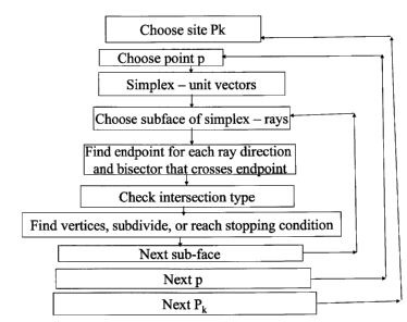
The method is shown in greater detail in Fig. 3C.
The system of equations may be of the form
B?. =H,
wherein:
m is the dimension of said region X;
0i, i=1,...,m are direction unit vectors;
p+Ti is the endpoint in direction 0i;
Ti T(Oi,p)0i is the vector whose direction is 0i and whose length is the
distance between point
p and endpoint p +T_i;
L i is the hyperplane corresponding to the endpoint p+Ti;
Ni is a normal to the hyperplane Li;
CA 02750093 2011-08-18
GAL235-1CA
is a vector of unknowns;
B is an m by m matrix with Bij =<Ni,Ti >, i,j=l,2,...,m; and
H=(H1,...,Hm) is the vector with Hi= <Ni,Ti >, i=1,2,...,m.
The method may further include:
5 computing respective vertices by solving the system of equations to obtain a
solution
and
checking if a corresponding vector u=p- 1T1+.AmTm, comprising the vectors
T1,...,Tm and the point p, is in the cone and in the cell, m being the
dimension of the region X,
which may typically be 2 or 3.
10 The region X may be of dimension two. In such a case the method may involve
dividing the given subface into additional subfaces. Dividing may involve
choosing an
intermediate vector between respective corners of the subface to create two
new subfaces,
where each new subface comprises the intermediate point and one of the
corners, or vectors in
a direction of the corners.
15 The region X may be of dimension two and deciding whether there are
vertices of the cell in
the cone generated by the endpoints may comprise checking one or more of:
a number of the hyperplanes,
whether there exist nonnegative solutions to the system of equations,
whether the determinant of matrix B vanishes or not,
20 whether there are infinitely many solutions, a unique solution or no
solution at all to
the system of equations.
Alternatively, the region X may be of dimension three. Dividing the given
subface into
additional subfaces may then involve dividing the subface into a partition of
additional
subfaces, where the partition is chosen from the following list of possible
partitions:
no partition at all,
a "small diameter partition",
"an interior point partition of type 0 ",
an interior point partition of type 1 ",
an interior point partition of type 2 ",
an interior point partition of type 3 ",
CA 02750093 2011-08-18
GAL235-1CA
21
"a boundary point partition of type 1 ",
"a boundary point partition of type 2 ", and
"a boundary point partition of type 3."
In the case of dimension three the stage of deciding whether there are
vertices of the
cell within the cone generated by the endpoints may comprises one or more of
the following:
checking the number of different hyperplanes,
checking whether there exist nonnegative solutions to the system of equations,
checking whether the matrix B is of rank 1, or rank 2, or rank 3, or of rank
smaller than
the rank of another matrix BH, or
checking whether there are infinitely many solutions, unique solution or no
solution at
all to the system of equations.
The computations would typically be carried out to a predetermined level of
error
parameters.
The method may reuse cell calculations of earlier stages for saving
calculations in later
stages.
Reference is now made to Fig. 3D, which is a simplified schematic flow chart
illustrating calculation of an endpoint. Computation of an endpoint in a given
direction 0 may
comprise selecting a point y along the corresponding ray in direction 0, and
moving and
testing y recursively, until a stopping condition is satisfied.
The stopping condition may, for example, comprise either using a result of a
distance
inequality, or testing whether a parameter is smaller than a given error
parameter. Recursive
testing may comprise selecting a point y along the ray emanating from p.
y may be on the boundary of region X or outside the cell of p. Now, if y is on
the
boundary, then one may define L as a corresponding hyperplane on which y is
located and
then check whether y is in the cell.
If y is in the cell, then one may select y as an endpoint and define L as the
corresponding bisecting hyperplane on which y is located.
If y is neither within the cell of p nor on a boundary of region X, then one
may find a
corresponding point closer to y than to p, and determine an intersection u
between the ray and
a corresponding hyperplane L. Then one may set y: =u, recursively testing
until y is in the cell
of p at which point one sets y as the endpoint. The corresponding point may be
a closest
CA 02750093 2011-08-18
GAL235-1CA
22
neighbor site or a point in the closest neighbor site, and L may be the
corresponding bisecting
hyperplane.
Reference is now made to Fig. 3E, which illustrates a method of storing
information
for the Vorronoi diagram. The method may involve retrieving combinatorial
information
related to the cells to a storage device, such as an electronic or magnetic
storage device, the
information including any combination of vertices, sides, faces (of any
dimension), neighbors
of a give vertex, the vertices of a given face in a desired order, and a
Delaunay graph. The
method may involve storing, in the storage device, for each desired site Pk
and each desired
point p, data related to any desired vertex u belonging to the cell of said p,
the data comprising
the coordinates of the vertex u, associated neighbor sites, associated
hyperplanes and
endpoints; and using the information to obtain information about the cells.
The method may involve applying the combinatorial information inter alia in
any of
the following applications: controlling or managing a communications network,
controlling or
managing a robot, modeling, testing, controlling or simulating a three-
dimensional network,
testing or modeling a material, data searching, searching for data on a
network or database,
image processing, mesh generation and re-meshing, curve and surface
generation, curve and
surface reconstruction, solid modeling, collision detection, controlling
motion of vehicles,
navigation, accident prevention, data clustering and data processing,
proximity operations,
nearest neighbor search, numerical simulations, weather prediction, analyzing
or modeling
proteins, analyzing or modeling crystal growth, analyzing or processing
digital or analog
signals, analyzing or modeling biological structures, designing drugs, finding
shortest paths,
pattern recognition, rendering, data compression, providing overall control of
a plurality of
methods for image processing, providing overall control of a plurality of
methods for data
categorization, providing overall control for a plurality of methods for data
clustering,
designing and testing of electronic circuits, management of geographic
information systems,
computing geometric objects, locating a resource according to the solution of
an efficient
location problem, face recognition, analyzing the behavior of populations,
analyzing or
modeling data related to astronomy, analyzing or modeling data related to
geography,
detecting or analyzing geometric structures, detecting or analyzing space
structures, location
based services, analyzing atmospheric data, analyzing oceanographic data,
detecting or
analyzing the distribution of matter in a region, detecting or analyzing the
distribution of
A_~v
CA 02750093 2011-08-18
GAL235-1CA
23
populations in a region, analyzing traffic, detecting or analyzing the
distribution of energy in a
region, and simply providing an artistic tool .
The method may comprise finding neighbor vertices of said vertex u with a
given
combinatorial representation by writing all vertices v for which m-1 of their
hyperplanes in
their combinatorial representation coincide with those of vertex u, in being
the dimension of
the region X.
The method may involve finding all the vertices on a given face corresponding
to a
given hyperplane L1.
Finding may involve:
determining all vertices v with Li in respective combinatorial representation;
finding all (m-2)-dimensional faces of said Ll by selecting an L_j, jai
belonging to a
vertex on Li, finding all vertices with Li and Lj in their combinatorial
representation, and
repeating the process with other Lj's; where in is the dimension of the region
X, as
before.
In an embodiment, the method may generate a convex hull from a collection of
sites by
selecting sites for which one of the faces of their cell is contained in the
boundary of the
overall region X .
The method may involve finding, from the stored data, different neighbors of a
site p;
computing therefrom a Delaunay tessellation; and passing an edge between a
site p and some
of its different neighbor sites.
. The Delaunay tessellation may be applied to any of the previously discussed
applications.
In the following, a schematic description of the first embodiment is
presented.
It is assumed that the distance used for the condition is the Euclidean
distance, that
there are finitely many sites, and that each of the sites consists of finitely
many points. This
allows one to treat sites with infinitely many points, such as balls or sites
with strange shape,
since each such site can be approximated to any required precision by a finite
subset of points.
The key ideas behind the method may be described in any dimension, and full
details will be
given later for dimension 2 and 3. See Figure 9 below for an illustration in
dimension 2.
CA 02750093 2011-08-18
GAL235-1CA
24
The method is based on the fact that under the above assumptions the cell of a
given point
p (belonging to some site Pk) is a convex polygon whose boundary consists of
vertices and
faces. See Figures 1 and 2. Despite the fact that the cell of a given site Pk
may not be convex
(see Figure 3), it can be computed by computing the cells of each of its
points p.
Referring again to Fig. 3B, the method may proceed as follows:
1. A site Pk and a point p in Pk are chosen. The goal is to compute the
Voronoi cell of p,
namely dom(p,Ak) where Ak is the union of all Pj, j :Ak.
2. Consider a simplex around p; The simplex is used in order to create the
unit vectors
and to obtain other information regarding the cell;
to 3. Choose a (sub)face of the simplex and create the unit vectors 01,...,8m
in the direction
of its corners. Then shoot rays in these directions ;
4. By taking into account the fact that the bisectors are (hyper)planes, for
each direction
01,...,O find its corresponding endpoint p+T(9i,p)8i and a corresponding
bisector Li
on which this endpoint is located;
5. By examining a certain system of equations, check what is the type of
intersection
between the detected hyperplanes;
6. Use the information obtained from the system of equations to decide whether
there are
vertices of the Voronoi cell in the (nonnegative) cone generated by the
endpoints, and
either find all of them (together with the hyperplanes on which they are
located),
possibly by further dividing the simplex (sub)face to subfaces, or reach a
stopping
condition for the current (sub)face and go to other (sub)faces.
7. The process continues until the treatment of all of the subfaces is
finished. In other
words, at each stage one finds all the possible vertices located in the part
of the space
"at which one looks", and the process ends when one finishes "covering" all
the space.
8. The above is repeated until dom(p,Ak) is computed for each desired point p
in Pk and
each desired site Pk.
The system of equations mentioned above is
BX.=H, (*)
CA 02750093 2011-08-18
GAL235-1CA
where:
the vector of unknowns is A A1,..., Am);
B is the in by in matrix whose components are Blj =<Ni,Tj >,
the components of the vector H=(Hi,...,Hm) are defined by Hi= < Ni,Ti >,
5 i,j=1,2,...,m, where Ti T(0i,p)0i denotes the vector in the direction of 0
whose length is the
distance from p to the endpoint, and Ni is a normal to the hyperplane
Lid x: <Ni,x>=ci= <Ni,p+Ti >} on which the endpoint p+Ti is located .
Equation (*) has the following simple geometric meaning:
the point
10 u9+(),1T1+...+ AmTm)
is in the intersection of the hyperplanes L1,...,Lm defined above if and only
if A solves this
equation. If one wants to restrict oneself to the cone generated by the
endpoints, then one
considers only the nonnegative solutions of equation (*), i.e., A_i > 0 for
all If
equation (*) has a unique nonnegative solution A, then this means that the
above vector u is a
15 point in the cone which is a candidate to be a vertex of the cell, since it
may be (but is not
necessarily) in the intersection of the corresponding in different faces
located on the
hyperplanes L1,...,Lm. If, in addition, u is found to be in the cell, then it
is indeed a vertex of
the cell.
A description for the case of dimension m=2 follows:
20 The method of Fig. 3B can be best understood in dimension m=2, and the
details are
given below. Things become more complicated for dimension m3, mainly because
of Stage 6
above. In order to find all the possible vertices in some part of the space
"viewed from p", one
takes into account many cases which do not occur in dimension 2, as will be
discussed in
greater detail hereinbelow.
25 A pseudo-code for the case m=2 is given. below. Reference is now made to
Fig. 9
which is a schematic illustration of the two-dimensional case. In Fig. 9, the
first subface is
represented by {01, 02}. The intersection of Ll and L2 is a point outside the
cone generated by
CA 02750093 2011-08-18
GAL235-1CA
26
the rays in the directions of 01, 02. The next two subfaces are {01, 03), {02,
03}. The cone
generated by the rays in the directions of 01, 04 is shown
In what follows the method and the pseudo-code will be explained in more
detail.
First, one creates the 3 unit vectors 0i corresponding to a simplex (a
triangle) around
the point p. After choosing a simplex subface, one shoots the two rays, and
finds the
corresponding bisecting lines Li. One wants to use this information for
finding all of the
possible vertices in the cone generated by the rays. By using equation (*) one
determines the
type of intersection between the lines L1,L2. The intersection is either the
empty set, a point,
or a line. The value of the determinant det(B) is used for distinguishing
between the cases.
If det(B) =0 and L1 =L2 (corresponding to the case where there are infinitely
many
solutions, i.e., the intersection is a line), then, as it can be easily
verified, there is no vertex of
the cell in the interior of the cone. Possibly one of the endpoints p+Ti is a
vertex, but this
vertex can be found with a different subface, and hence one can finish with
the current subface
and proceed to the other subfaces.
If det(B) =0 and L16L2 (corresponding to the case where there is no solution
of any
kind, including solutions which are not non-negative, i.e., the intersection
is the empty set),
then one does not have enough information to decide if the cone corresponding
to the current
simplex subface contains vertices of the cell, and hence one divides this
subface into two
(equal) subfaces and continues the process with each of these subfaces.
If det(B)#0 (corresponding to the case where there exists a unique solution
X=(X1'X2)
then two possibilities may occur. In the first, X is not nonnegative, i.e.,
u=p41T1 +1,2T2 is not
in the cone, and in this case one does not have enough information about
possible vertices in
the cone so one divides the current subface into subfaces and continues the
process.
Otherwise, ? is nonnegative, i.e., u is in the cone. If u is in the cell
(something which can be
checked, for instance, by distance comparisons), then it is a vertex and one
stores the vertex
together with any other relevant data such as the corresponding lines and so
on as discussed in
greater detail hereinbelow. After storing u one has finished with the current
subface and can
CA 02750093 2011-08-18
GAL235-1CA
27
proceed to the other subfaces. Otherwise (i.e., u is outside the cell) u is
not a vertex, and one
has actually found a new line corresponding to the ray in the direction
03: =(u-p)/ i-p j. One divides the current subface using 83 and continues the
process.
From the above description it seems that the method should be implemented in a
recursive way. However, by using a simple data structure, herein referred to
as FaceList, one
can avoid the need to use a recursive implementation and instead can use
loops. The reason
that this is possible is because the treatment of each subface can be carried
out independently
of the other subfaces, including its "parent"' or "children": no information
is exchanged
between the subfaces. As a result, one can maintain a list of subfaces, the
FaceList - in which
each subface is represented by a set of two unit vectors, which correspond to
its corners, and
run the process until the list is empty. The initial list contain the faces of
the simplex , namely
IT 1, (P2},
{T2, T3}, and {TI, T3}, where one can take TI=(0.5. 3,-05), q =(0,1),
T3=(-0.5-43,-0.5).
In this connection it may be emphasized that the simplex is used,
conceptually, for creating the
unit vectors, but these unit vectors are only in the direction of the corners
of a given subface,
and they are not necessarily on the same line as the one on which the subface
is located.
Despite this, it is convenient to represent a subface by its associated unit
vectors .
A pseudocode for the method in dimension 2:
Input: The sites.
Output: The Voronoi cells.
1. Create the simplex unit vectors and call them Ti, 14,2,3;
2. For each desired site Pk do
3. For each desired point p in Pk do
4. Create the initial faces and enter them into FaceList;
5. Let fl be the index running on FaceList;
6. Let Oi pi, i=4,2 and fl =4 01,02}; [simply an initialization)
7. While FaceList is nonempty do
CA 02750093 2011-08-18
GAL235-1CA
28
8. Denote Ti T(0i,p)0i and compute the endpoints p+Ti, i4,2;
9. Find a (closest) neighbor site gi, i=4,2 (or a point in it if a site
has more than one point) to p+Ti;
10. Compute the bisecting line Li between p and g i , i =4,2.
If no g i exists for some i, then p+Ti, is on the boundary of the world. 5
Call Li to the corresponding boundary line;.
11. Consider the system of equations (*)
12. If det(B) =0 then [no solution or infinitely many]
13. If Ll =L2 then [no vertices in this cone; we are done]
14. Remove {01,02} from FaceList;
15. Assign to fl the next element in FaceList;
16. Else [not enough information (no solution), so
continue]
17. Define 03 X01 -+02)/ P 1402 [i =e =, (01402)12
normalized]
18. Enter the subfaces {01, 03), 102, 03) into FaceList;
19. Remove {01,02} from FaceList;
20. fl 102, 03) ; [just a new initialization]
21. Else [i.e., det(B) # 0, namely a unique solution )j
22. If X is nonnegative then [we are in the nonnegative
cone]
23. Let up-I;,1T1+?2T2;
24. If u is inside the cell of p then
25. Store u; [u is a vertex of the cell. We are
done]
26. Remove {01,02) from FaceList;
27. Assign to fl the next element in FaceList;
CA 02750093 2011-08-18
GAL235-1CA
29
28. Else [u is outside the cell. We continue]
29. Let 03 (u-p)/ )u-p ~
30. Create the (at most) 2 subfaces 101, 03),
{02, 03} and
enter them into FaceList;
31. Remove {01,02} from FaceList;
32. fl 402, 03) ; [just a new initialization]
33. Else [u is not in the cone. Not enough
information]
34. Define 03 401 -102)/ P14021 [i.e., (01402)/2
normalized]
35. Enter the subfaces {01, 03), {02, 03} into
FaceList;
36. Remove ( 01,02) from FaceList;
37. fl =1 02, 03} ; [just a new initialization]
Finding the endpoints exactly
In order to apply the above method, one should be able to find the endpoint
p+T(O_i,p)O_i. One possible method is to use the method disclosed in US Patent
Application
No. 12/461,216, but the problem is that the endpoint found by this method is
approximated: it
is given up to some error parameter, and unless this parameter is very small,
this may cause an
accumulating error later when finding the sides and vertices, due to numerical
errors in the
expressions in equation (*).
In what follows a further method will be described for finding precisely the
endpoint in a
given direction 0. Of course, when using floating point arithmetic errors
appear, but they are
much smaller than the ones described above. The method can be implemented in
any
dimension. Reference is made to Figure 10 for an illustration in dimension 2.
Specifically, Fig.
10 shows a schematic illustration of the method for finding the endpoint of a
given ray. The
CA 02750093 2011-08-18
GAL235-1CA
dimension of the world is 2. The ray comes from far away. At the first
displayed iteration
CloseNeighbor is al. The intersection between the corresponding line L1 and
the ray is u =u1
. At the next stage CloseNeighbor is a2 and u =u2. The process ends since u2
is in the cell of
p, i.e., u2 is the endpoint. More details about certain steps are mentioned in
later sections.
5
method:Endpoint:
1. Shoot a ray in the direction of 0 and stop it at a point y which is either
in the region X
but outside the cell of p, or it is the intersection of the ray with the
boundary of the
region. If y is choosen to be outside the cell then go to Step 4. Otherwise,
let L be the
10 boundary hyperplane on which y is located.
2. Check whether y is in the cell of p, e.g., by comparing d(y,p) to d(y,a)
for any a in the
other sites, possibly with enhancements. A possible way for accelerating the
computation is, each time when it is found that d(y,p)<_d(y,a) for some a,
then a can be
removed from the list A of points in the other sites, since it will always be
the case that
15 also later (for later values of y along the ray) the inequality
d(y,p)<d(y,a) will hold.
3. If y is in the cell, then y is the endpoint and L is the bisecting
hyperplane. The
calculation along the ray is complete.
4. Otherwise, d(y,a) 41(y,p) for some a in some (different) site. Let
CloseNeighbor: =a.
5. Find the point of intersection (call it u) between the given ray and the
bisecting
20 hyperplane L between p and CloseNeighbor. This intersection is always
nonempty.
The hyperplane is easily found because it is vertical to the vector p-
CloseNeighbor
and passes via (p -CloseNeighbor)/2.
6. Let y: =u. Go to Step 2.
25 A more detailed description of the method of Fig. 3B is now provided for
the case of
dimension m3.
Here the dimension of the world X is m=, and a 3-dimensional simplex is used
as an
aid for creating the unit vectors and gaining information regarding the
vertices and faces of the
Voronoi cell. As in the case of dimension mom, one can implement this method
using loops
30 instead of recursion, using the data structure called FaceList, with the
difference that now, in
the three-dimensional case, each subface is represented by a set of three unit
vectors, which
CA 02750093 2011-08-18
GAL235-1CA
31
are in the direction of its corners. The structure is simply a list of
subfaces, and the process
runs until the list is empty. The initial list contains the faces of the
simplex.
Reference is now made to Figures 11 - 18, which illustrate various aspects of
the
Voronoi diagram calculation for the three-dimensional case.
Figure 11 shows a small diameter partition of a subface of a 3D simplex and
its sub-
faces, for the method of Fig. 3B for computing the Voronoi cells in the 3-
dimensional case.
Figure 12 shows an example of a boundary point partition of type 1 of a
subface of a
3D simplex and its sub-faces for the method of Fig. 3B in the 3-dimensional
case. There are 2
subfaces, and in this example ul is outside the cell.
Figure 13 shows an example of a boundary point partition of type 2 of a
subface of a
3D simplex and its sub-faces for the method of Fig. 3B in the 3-dimensional
case. There are 3
subfaces. In this example u1 and 113 are outside the cell.
Figure 14 shows an example of a boundary point partition of type 3 of a
subface of a
3D simplex and its sub-faces for the method of Fig. 3B in the 3-dimensional
case Here u1, 112
,
and 113 are outside the cell.
Figure 15 shows an example of an interior point partition of type 0 of a
subface of a 3D
simplex and its sub-faces for the method of Fig. 3B in the 3-dimensional case.
Figure 16 shows an example of an interior point partition of type 1 of a
subface of a 3D
simplex and its sub-faces for the method of Fig. 3B in the 3-dimensional case.
In this example
u l is outside the cell.
Figure 17 shows an example of an interior point partition of type 2 of a
subface of a 3D
simplex and its sub-faces for the method of Fig. 3B in the 3-dimensional case.
In this example
u1 and u3 are outside the cell.
Figure 18 shows an example of an interior point partition of type 3 of a
subface of a
3D simplex and its sub-faces for the method of Fig. 3B in the 3-dimensional
case. In this
example ul, u2, and u3 are all outside the cell.
In all of these figures a face of a 3-dimensional simplex is shown (as seen
from above)
and it is partitioned into several subfaces, according to the specific case it
treats. Each such
partition has a name which is used below, e.g., "an interior point partition
of type P. It should
CA 02750093 2011-08-18
GAL235-1CA
32
be emphasized again that the simplex is used (conceptually) for creating the
unit vectors, but
these unit vectors are only in the direction of the corners of a given
subface, and they are not
necessarily on the same plane as the one on which the subface is located.
Despite this, it is
convenient to represent a subface by its associated unit vectors .
The following terminology is used: when a certain partition (e.g., "a small
diameter
partition') is applied to some given subface F, then one is done with F and
continues with the
other subfaces.
A pseudocode method for the 3D case is as follows:
1. Create the simplex unit vectors and call them (pi, i==1,2,3,4;
Create the simplex faces;
2. Repeat the following (until the end) for each desired site Pk and each
desired point p in Pk.
3. Enter the simplex faces into FaceList;
4. Let Oi Bpi, i =4,2,3 and choose the face F =4 01,02,031; [simply an
Initialization]
5. Repeat the following (until the end) while FaceList is nonempty:
6. If det(01, 02, 03) =O, then we are done with the face F, i.e., remove F
from
FaceList [because F is degenerate]; Continue with the next subface in
FaceList;
7. Else (until the end), let Ti T(9i,p)6i; Compute the endpoints p+Ti,
i=4,2,3; Find a neighbor
site gi, i=4,2,3 (or a point in it if a site has more than one point) to p+Ti;
Compute the
bisecting plane Li between p and gi, i=4,2,3;
If no gi exists for some i, then p +Ti is on the boundary of
the world. Call Li to the corresponding boundary plane;
8. Check the real number of planes by checking if the 3 endpoints are on the
same plane (e.g.,
by checking if p +Ti, i ,3 are on L2), or on 2 different planes, or on 3
different planes [to
avoid problems later, since a point can be on several planes]; Change the
planes Li
associated with p +Tiaccordingly;
9. Let BH be the matrix composed of B with an additional (right) column H
(where H is
defined after equation (*) ), and consider equation (*).
CA 02750093 2011-08-18
GAL235-1CA
33
10. If rank(B) 4ank(BH) [no solutions to equation (*), namely not enough
information
regarding possible vertices in the cone], then make a
"small-diameter partition" of F; Enter the resulting subfaces into FaceList
and
remove F from it; We are done with F;
11. Else (until the end), from now on rank(B) =rank(BH), and
there are three possible cases:
12. Case 1, rank(B) 4: [in this case all the planes are the same]
Check if one of the endpoints p+Ti, i4,2,3 is a vertex by checking if it was
obtained by at least 3 bisecting planes (including the faces of the boundary
of
world if it is on such faces) , and if yes, then store it; We are done with F
anyway (even if
the endpoints are not vertices);
13. Case 2, rank(B) =2:
This case happens only when two planes are the same and the
third is different. By stage 8 the endpoint corresponding to the different
plane
is not on the same plane as the other two endpoints .
A. Check if one of the endpoints p+Ti, i=4,2,3
is a vertex by checking if it was obtained by at least 3
bisecting planes (including all the faces of of the boundary of
the world if it is on such faces), and store it if yes .
B. Put X 1 =0, and check whether the system (*) has a nonnegative solution of
the form (0, X2, X3), i.e., one needs to solve a system of two
unknowns and two equations (recall that in the canonical form of the
matrix
the third equation is 0 =0 ) [Geometric meaning: the line of intersection A
of the two planes L2, L3 passes via the face X1 =0 of the cone].
Check also if there are nonnegative solutions of the form (X1,0, X3)
and (X1,1,2,0). Let NumLambda be the number of all of these solutions.
C. If NumLambda=0, then there is no nonnegative solution of the above form.
Make
a "small diameter partition" of F [the line A is not in the cone:
CA 02750093 2011-08-18
GAL235-1CA
34
not enough information] and continue with these subfaces;
D. Else, from now on NumLambda ). Let (?.1 ? 2,X3) be a nonnegative
solution corresponding to some Xi=O, and let ui = p4kjT1-2T2- 3T3
check whether ui is in the Voronoi cell of p, and along the way find
all the bisecting planes corresponding to ui; If ui has at least 3bisecting
planes, then ui is a vertex. In this case store ui;
Now there are several possible sub-cases:
a) NumLambda 1:
i. If (the unique) ui is in the cell ,
then make a "small diameter partition" of F.
ii. Else, make a "boundary point partition of type 1" of F corresponding
to ui;
b) NumLambda 3 :
i. If the two ui are the same, then go to the case NumLambda =1.
ii. If both of the two different ui are in the cell of p, then we are
done with the face F .
iii. If both of the two different u_i are outside the cell of p
then make a "boundary point partition of type 2" of F corresponding to
these ui;
iv. If there is one uk in the cell of p and one different ui outside the cell,
then
make a "boundary point partition of type 1" of F corresponding to
ui ;
c) NumLambda --3: it must be that among the ui, Uj, Uk , two are the same, and
they are different from the additional one.
Hence this is actually the case NumLambda=2, and so
(after finding the two different ones) do what written there;
CA 02750093 2011-08-18
GAL235-1CA
14. Case 3, rank(B)3:
The system (*) has a unique solution X=(?1, X2),3)=
If X is not nonnegative, then make a "small diameter partition" of F;
5 Else, from now on ? is nonnegative. Let u=p-I gT1-1 2T24?3T3;
Check whether u is inside the Voronoi cell of p and along the way find all the
bisecting
planes corresponding to u.
A. If u is not inside the cell of p (also in the case where u is outside the
world), then u
is not a vertex of the cell;
10 Make an "interior point partition of type 0" of F.
B. Else, from now on u is inside the cell, and hence u is a vertex of the
cell, but
additional checks are needed for not missing other vertices corresponding to
F;
Store U;
C. Let S1 be the intersection of L2, L3, let S2 be the intersection of L3 and
L1, and let
15 S3 be the intersection of L1 and L2;
Each Si is a line which has the parametric representation
{u-ttQi : t is real} where Qi is the cross product of Nj and Nk , isj,k
are all different, and Nj is the normal to the plane Lj;
Find the point of intersection ui=u-ftQi of Si and the plane which passes via
p
20 whose normal M is the cross product of Tj and Tk; [this is the plane
passing via p
and generated by Tj,Tk. The formula for t is
t = I-u,M -'4(-N,Qi >)l
D. Check whether ui p is in the non-negative cone generated
by T1,T2,T3; Let NumU be the number of ui such
25 that both ui p is in the non-negative cone generated by T1,T2,T3
and that ui is outside the Voronoi cell of p (along the way find all the
bisecting
CA 02750093 2011-08-18
GAL235-1CA
36
planes corresponding to ui; for checking if ui-p is in the nonnegative cone
generated by T1,T2,T3 it suffices to check
that ui-p is in the nonnegative cone generated by Tj,Tk, where
j,k are different from i, and this may be done by checking if a corresponding
linear
system has a nonnegative solution); For any ui which is inside the cell and
has at
least 3 bisecting planes, store ui;
E. If all the 3 points ui are inside the cell of p and all the 3 points
ui p, i---i,2,3 are in the nonnegative cone generated by T1,T2,T3,
then we are done with F; [there are no other vertices
corresponding to F]
F. Else,
a) If NumU==1,2 or 3, then
i. If u =lj for j =4,2 or 3 (one of the corners of the subface F), then make a
'
'boundary point partition of type NumU" of F corresponding to the above
points ui associated with NumU;
ii. Else, make an "interior point partition of type NumU" of F
corresponding to above points ui associated with NumU;
b) Else
i. If u=Oj for j ,2 or 3, then make a make
"a small diameter partition" of F.
ii. Else, make "an interior point partition of type O"of F.
Storing the data and obtaining combinatorial information and additional
information
The following explains schematically how the data may be stored, with
reference again
to Fig. 3E, and how to retrieve combinatorial information and additional
information related to
the Voronoi cells and more. Here the dimension of the region X can be general.
Given a point p in some site Pk, when a vertex u from the cell of p is found,
one stores
the following features: its coordinates, the hyperplanes from which it was
obtained (i.e., u
CA 02750093 2011-08-18
GAL235-1CA
37
belongs exactly to the corresponding faces located on these hyperplanes), the
point p and the
index k. For storing a hyperplane L it is convenient to store the index of its
associated
neighbor site, namely the index (number) of the site which induces it. If it
is a boundary
hyperplane, then it has a unique index number which is stored and from this
index one can
retrieve the parameters (the normal and the constant) defining the hyperplane.
Alternatively,
these parameters can be stored directly. For some purposes it may be useful to
store also some
endpoints associated with each hyperplane. A convenient data structure for
storing the whole
diagram is a two dimensional array, indexed by p and k, in which the vertices
(represented, as
explained above, by coordinates and associated neighbor sites) and any
additional information,
such as endpoints, are stored.
If one wants to compare two hyperplanes, then one can simply compare the index
of
the associated neighbor site/boundary hyperplane. If one needs additional
information on the
hyperplane, then this information can be retrieved immediately because the
hyperplane is
perpendicular to the segment [pa] and passes via the middle point of this
segment (a is the
given neighbor); in the case of a boundary hyperplane from its index one
retrieves the
parameters which are stored in a different list.
In dimension m=2 a vertex is always obtained from 2 lines. In dimension m?3 a
vertex
is usually obtained from exactly m hyperplanes, but in principle it can be
obtained from S
hyperplanes, where S>m. The set L_{ i_S}} of all the hyperplanes from which u
was obtained is referred to herein as the combinatorial representation of u.
As the examples below show, once the above information is stored, one can
obtain any other
combinatorial information related to the cell of p, say the neighbors of a
given vertex, the
edges of some cell, and so on, and hence one does not need to store these
types of data
separately. This is in contrast to familiar methods of representing a
combinatorial information
related to the Voronoi diagram, in which one has to find and store all the j-
dimensional faces,
j=0,1, ...,m-1 of the cell.
Example 1:
The neighbors (in the same cell) of some given vertex u with a given
combinatorial
representation are all the vertices v for which m-1 of their hyperplanes in
their combinatorial
representation coincide with those of u.
CA 02750093 2011-08-18
GAL235-1CA
38
Example 2:
Given some hyperplane Li, all the vertices v with Li in their combinatorial
representation are the vertices of the face of the cell of p corresponding to
Li (i.e., this face is
located on Li). This face is denoted by Li again. This is an (m-1)-dimensional
polygon.
Suppose one wants to find all the (m-2)-dimensional faces of Li. One chooses
some Lj, jai
belonging to some vertex on Li, and looks at all the vertices with Li and Lj
in their
representation. These vertices create an (m-2)-dimensional face of Li, and by
repeating the
process with the other Lj's one finds all the other (m-2)-dimensional faces.
In general, given
some different hyperplanes all the vertices with in
to their representation create an (m-S)-dimensional face of the cell.
Example 3:
Given the vertices of a two dimensional face (possibly in a three dimensional
cell),
suppose one wants to arrange them in counterclockwise order. Let ul be some
vertex with
{Lj,Lj} as its representation. One finds the other vertex u2 with Lj in its
representation. Suppose that {Lj,Lk} is the representation of u2. One then
finds the other
vertex 113 with Lk in its representation and so on. One now has a list
ul,...,uN of all the
vertices of the cell in either clockwise or counterclockwise order. To decide
which order was
obtained one can check the sign of the expression D1iet(ul-u2,u2-u3): if Dom,
then this a
counterclockwise order, and if D m, then this is a clockwise order (and hence
one reverses the
order of the list of vertices).
Example 4: When the two dimensional face in the method described in a previous
example is
the cell itself, another method can be used in order to obtain a
counterclockwise order. One
gives a sorting value to each endpoint and at the end sorts the vertices in
increasing or
decreasing order according to their sorting value. The sorting value is
obtained as follows: the
CA 02750093 2011-08-18
GAL235-1CA
39
3 initial directions (pi, i =1, 2, 3 have the sorting values 1,2,3
respectively. Then, if 01 and 02
are two directions from which an intermediate unit vector 03 is created, then
the sorting value
s3 of 03 is defined as
s3. =(si +s2)/2 where si is the value associated with 0i, i ==1,2 (or another
an intermediate value
between s1 and s2).
Example:
Suppose that the sites are points. Given a vertex u in the cell of some site
Pk, for
finding all of its neighbor vertices in the entire diagram one may proceed by
finding all the
vertices v in the entire diagram for which (m-1) of the hyperplanes in their
representation
coincide with those of u.
Example:
The convex hull of a set of points is the minimal convex set which contains
them.
Suppose that the sites are points. The convex hull can be generated by a
subset of the given
sites composed of all the sites whose cells are not bounded. Hence, to find
all the generating
sites one needs to take a large enough region X and to check all the sites
whose cells contain a
face which is on the boundary of X. After finding these sites one knows that
they are on the
boundary of the convex hull and the rest of the sites are in the interior of
the convex hull.
Example:
Once the faces are known, one can represent the cells using many endpoints by
adding
them in a fast way. Suppose one wants to add r>1 endpoints on each face.
1. If the dimension in is 2: suppose that Lax: N,x> =c) is the line on which
the face is
located, and let p+T_1, p+T_2 be the corners of the face. For any j, 1:5j4,
let
W_j =(T_1-f(j/r)(T_2-T 1))/~_1-f(j/r)(T 2-T_ 1) land
tic- 'N,p~/( 'N,(pj>). The point p+t=(pJj is an endpoint located on the given
face.
2. If in >2: Let L =(x: N,x > = c) be the (hyper)plane on which the face is
located. For each
i= 1,...,m and each j, 1<j 4 do the following:
Let D_i=(T_1+...+T_m)-T_i.
CA 02750093 2011-08-18
GAL235-1CA
Let S
~(1-(j/r))/(m-1))D_i,
Let cp_ij =((j/r)T_i +S)/ Kj/r)T_i +S
[interpretation: a (normalized) convex combination of T i and the center of
mass
of the other T j].
5 Add the endpoint p+t=cp_ij, where tic- cN,p>)/(dv,(p_ij >).
Computing the Delaunay graph (Delaunay tessellation)
Referring now to Fig. 19 and also to the flow chart of Fig. 3F, here it is
explained how
to compute the Delaunay graph (the Delaunay tessellation) of the given sites.
The Delaunay
10 tessellation is an important geometric structure which by itself has many
applications.
Suppose that the sites P1,...,Pn are points. By definition, the Delaunay graph
consists
of vertices and edges. The vertices of the Delaunay graph are the sites. There
is an edge
between two sites if their Voronoi cells are neighbors (via a face). Fig. 19
illustrates the graph
in dimension 2 .. The Delaunay graph shown is of 20 sites in the plane (thick
line). The
15 Voronoi cells of the same sites are shown as well in thin line.
As a result, for computing the Delaunay graph one chooses a given site, goes
over the
data structure used for storing the Voronoi cells as explained hereinabove,
and finds all the
different neighbor sites of a given site. The procedure is repeated for each
site .For drawing
the Delaunay graph one simply connects two sites by an edge when it is found
that one site is
20 a neighbor site to another one .
Additional notes
In this section the following additional notes relate to the implementation of
the methods
described hereinabove.
1. If the world X is a polygon, then the intersection of some ray in the
direction of 0 with the
boundary (needed in Method:Endpoint)), can be easily found. One simply goes
over the
faces of the world (the i-th face is represented as
'i,x > zi) and check if p -+tO is on the i-th face by checking if both
t =(ci iP N ,0 >) is positive and p -It0 is in the world. The process stops at
the first
face satisfying the above.
CA 02750093 2011-08-18
GAL235-1CA
41
2. If some site Pk has more than one point, then one treats each of the cells
of its points
separately. There are situations in which one wants to consider only points
which are on
the boundary of the Voronoi cell of Pk. In particular, one has to be sure to
remove vertices
which are actually internal points. Here is a simple way to check if a point
E=p-ft0 which
is known to be an endpoint (e.g., a vertex) is on the boundary of the cell
when Pk has more
than one point: one compares t l(E,p) to d(E,q) for any q in Pk. If t Q1(E,q)
for some q,
then E is not a boundary point. Otherwise E is a boundary point.
3. The initial unit vectors: in dimension in =2 they can be taken as
(p1=(0.5'J3; 0.5), 92=0,1), (P3=(-0.5.I3; 0.5). In dimension m3 they can be
taken as
(P1 41,0,0), tP2=(-1/3, (i8)/3,0), (3=(-1/3,-(i2)/3,('.16)/3),
(P4=(-l/3,-(12)/3; ('16)/3).
4. One should go over the final list of vertices to check for redundancy,
because a vertex may
be found more than one time .
5. Error parameters: for significantly reducing problems related to numerical
errors, it is
recommended to use error parameters. Here are some examples:
a) When checking if two real numbers a and b are identical, one checks whether
ta-
b t<1 for some small error parameter 61. Similary, when checking if two
vectors a
and b are identical, we check if the norm
to-b t<P-2, where one can take the Euclidean norm, the max norm or any other
norm.
b) When checking if a 3 by 3 matrix in the canonical form has rank 2, one can
check
whether the norm tR I of the third line R satisfies . t<e3.
c) When checking if the components ki of X=(X1,X2)3) are nonnegative, one
first
checks whether ~i t<t.4 for some i, and if yes, then regards this X, as 0.
CA 02750093 2011-08-18
GAL235-1CA
42
d) For checking if some determinate D vanished, one checks if P I<85.
All of these parameters si are quite small (say 10A{-7} or 10"{-10}), but they
are not
necessarily identical, and their magnitude may change according to the
floating point
arithmetic and the number of sites.
6. To check if a vertex v (or an endpoint) is obtained by more than 3 planes
the following
procedure can be used: d(v,p) and d(v,a) are compared for any a in the other
sites(possibly
using enhancements ); then all the points a satifying d(v,a)= l(v,p) are
stored. If eventually
d(v,p)5d(v,a) for any a, then those points a satisfying d(v,a) =d(v,p) are the
neighbors of v,
and the corresponding bisectors between those a and p are the planes from
which v was
obtained. This can be done during finding the endpoint (Method:Endpoint)), in
the
corresponding step in which a similar comparison is made .
7. Many calculations, e.g., the computation of endpoints, vertices or faces
can be saved
because they have already been made in previous stages of the computation (of
a certain
cell or previous cells).
It is appreciated that certain features of the invention, which are, for
clarity, described
in the context of separate embodiments, may also be provided in combination in
a single
embodiment. Conversely, various features of the invention, which are, for
brevity, described
in the context of a single embodiment, may also be provided separately or in
any suitable
subcombination.
Although the invention has been described in conjunction with specific
embodiments
thereof, it is evident that many alternatives, modifications and variations
will be apparent to
those skilled in the art. Accordingly, it is intended to embrace all such
alternatives,
modifications and variations that fall within the spirit and broad scope of
the appended claims.
In addition, citation or identification of any reference in this application
shall not be construed
as an admission that such reference is available as prior art to the present
invention.