Note: Descriptions are shown in the official language in which they were submitted.
CA 02842932 2014-01-23
WO 2013/015851
PCT/US2012/032623
SYSTEM FOR ESTIMATING POWER DATA FOR A PHOTOVOLTAIC POWER
GENERATION FLEET
This invention was made with State of California support under Agreement
Number 722.
The California Public Utilities Commission of the State of California has
certain rights to this
invention.
TECHNICAL FIELD
This application relates in general to photovoltaic power generation fleet
planning and
operation and, in particular, to a computer-implemented system and method for
estimating power
data for a photovoltaic power generation fleet.
BACKGROUND ART
The manufacture and usage of photovoltaic systems has advanced significantly
in recent
years due to a continually growing demand for renewable energy resources. The
cost per watt of
electricity generated by photovoltaic systems has decreased dramatically,
especially when
combined with government incentives offered to encourage photovoltaic power
generation.
Photovoltaic systems are widely applicable as standalone off-grid power
systems, sources of
supplemental electricity, such as for use in a building or house, and as power
grid-connected
systems. Typically, when integrated into a power grid, photovoltaic systems
are collectively
operated as a fleet, although the individual systems in the fleet may be
deployed at different
physical locations within a geographic region.
Grid connection of photovoltaic power generation fleets is a fairly recent
development.
In the United States, the Energy Policy Act of 1992 deregulated power
utilities and mandated the
opening of access to power grids to outsiders, including independent power
providers, electricity
retailers, integrated energy companies, and Independent System Operators
(IS0s) and Regional
Transmission Organizations (RT05). A power grid is an electricity generation,
transmission, and
distribution infrastructure that delivers electricity from supplies to
consumers. As electricity is
consumed almost immediately upon production, power generation and consumption
must be
balanced across the entire power grid. A large power failure in one part of
the grid could cause
electrical current to reroute from remaining power generators over
transmission lines of
insufficient capacity, which creates the possibility of cascading failures and
widespread power
outages.
CA 02842932 2014-01-23
WO 2013/015851
PCT/US2012/032623
As a result, both planners and operators of power grids need to be able to
accurately
gauge on-going power generation and consumption, and photovoltaic fleets
participating as part
of a power grid are expected to exhibit predictable power generation
behaviors. Power
production data is needed at all levels of a power grid to which a
photovoltaic fleet is connected,
especially in smart grid integration, as well as by operators of distribution
channels, power
utilities, IS0s, and RT0s. Photovoltaic fleet power production data is
particularly crucial where
a fleet makes a significant contribution to the grid's overall energy mix.
A grid-connected photovoltaic fleet could be dispersed over a neighborhood,
utility
region, or several states and its constituent photovoltaic systems could be
concentrated together
or spread out. Regardless, the aggregate grid power contribution of a
photovoltaic fleet is
determined as a function of the individual power contributions of its
constituent photovoltaic
systems, which in turn, may have different system configurations and power
capacities. The
system configurations may vary based on operational features, such as size and
number of
photovoltaic arrays, the use of fixed or tracking arrays, whether the arrays
are tilted at different
angles of elevation or are oriented along differing azimuthal angles, and the
degree to which each
system is covered by shade due to clouds.
Photovoltaic system power output is particularly sensitive to shading due to
cloud cover,
and a photovoltaic array with only a small portion covered in shade can suffer
a dramatic
decrease in power output. For a single photovoltaic system, power capacity is
measured by the
maximum power output determined under standard test conditions and is
expressed in units of
Watt peak (Wp). However, at any given time, the actual power could vary from
the rated system
power capacity depending upon geographic location, time of day, weather
conditions, and other
factors. Moreover, photovoltaic fleets with individual systems scattered over
a large
geographical area are subject to different location-specific cloud conditions
with a consequential
affect on aggregate power output.
Consequently, photovoltaic fleets operating under cloudy conditions can
exhibit variable
and unpredictable performance. Conventionally, fleet variability is determined
by collecting and
feeding direct power measurements from individual photovoltaic systems or
equivalent indirectly
derived power measurements into a centralized control computer or similar
arrangement. To be
of optimal usefulness, the direct power measurement data must be collected in
near real time at
fine grained time intervals to enable a high resolution time series of power
output to be created.
However, the practicality of such an approach diminishes as the number of
systems, variations in
system configurations, and geographic dispersion of the photovoltaic fleet
grow. Moreover, the
costs and feasibility of providing remote power measurement data can make high
speed data
- 2 -
CA 02842932 2014-01-23
WO 2013/015851
PCT/US2012/032623
collection and analysis insurmountable due to the bandwidth needed to transmit
and the storage
space needed to contain collected measurements, and the processing resources
needed to scale
quantitative power measurement analysis upwards as the fleet size grows.
For instance, one direct approach to obtaining high speed time series power
production
data from a fleet of existing photovoltaic systems is to install physical
meters on every
photovoltaic system, record the electrical power output at a desired time
interval, such as every
seconds, and sum the recorded output across all photovoltaic systems in the
fleet at each time
interval. The totalized power data from the photovoltaic fleet could then be
used to calculate the
time-averaged fleet power, variance of fleet power, and similar values for the
rate of change of
10 fleet power. An equivalent direct approach to obtaining high speed time
series power production
data for a future photovoltaic fleet or an existing photovoltaic fleet with
incomplete metering and
telemetry is to collect solar irradiance data from a dense network of weather
monitoring stations
covering all anticipated locations of interest at the desired time interval,
use a photovoltaic
performance model to simulate the high speed time series output data for each
photovoltaic
system individually, and then sum the results at each time interval.
With either direct approach, several difficulties arise. First, in terms of
physical plant,
calibrating, installing, operating, and maintaining meters and weather
stations is expensive and
detracts from cost savings otherwise afforded through a renewable energy
source. Similarly,
collecting, validating, transmitting, and storing high speed data for every
photovoltaic system or
location requires collateral data communications and processing
infrastructure, again at possibly
significant expense. Moreover, data loss occurs whenever instrumentation or
data
communications do not operate reliably.
Second, in terms of inherent limitations, both direct approaches only work for
times,
locations, and photovoltaic system configurations when and where meters are
pre-installed; thus,
high speed time series power production data is unavailable for all other
locations, time periods,
and photovoltaic system configurations. Both direct approaches also cannot be
used to directly
forecast future photovoltaic system performance since meters must be
physically present at the
time and location of interest. Fundamentally, data also must be recorded at
the time resolution
that corresponds to the desired output time resolution. While low time-
resolution results can be
calculated from high resolution data, the opposite calculation is not
possible. For example,
photovoltaic fleet behavior with a 10-second resolution can not be determined
from data
collected by existing utility meters that collect the data with a 15-minute
resolution.
The few solar data networks that exist in the United States, such as the ARM
network,
described in G.M. Stokes et al., "The atmospheric radiation measurement (ARM)
program:
- 3 -
CA 02842932 2015-10-01
WO 2013/0I585I P(717E:S2012/032623
programmatic background and design of the cloud and radiation test bed,"
Bulletin of Am.
Meteorological Society 75, 1201-1221 (1994),
and the SURERAD network, do not have high density networks (the closest pair
of
stations in the ARM network is 50 km apart) nor have they been collecting data
at a fast rate (the
fitstest rate is 20 seconds at ARM network and one minute at SURFRAD network).
The limitations of the direct measurement approaches have prompted researchers
to
evaluate other alternatives. Researchers have installed dense networks of
solar monitoring
devices in a few limited locations, such as described in S. Kuszamaul et al.,
"Lanai High-Density
Irradiance Sensor Network for Characterizing Solar Resource Variability of MW-
Scale PV
System." 35" Photovoltaic Specialists Conf., Honolulu, Ill (June 20-25, 2010),
and R. George,
"Estimating Ramp Rates for Large PV Systems Using a Dense Array of Measured
Solar
Radiation Data," Am. Solar Energy Society Annual Conf. Procs., Raleigh, NC
(May 18, 2011).
As data are being collected, the
researchers examine the data to determine if there are underlying models that
can translate results
from these devices to photovoltaic fleet production at a much broader area,
yet fail to provide
translation of the data. In addition, half-hour or hourly satellite irradiance
data for specific
locations and time periods of interest have been combined with randomly
selected high speed
data from a limited number of ground-based weather stations, such as described
in CAISO 2011.
"Summary of Preliminary Results of 33% Renewable Integration Study ¨ 2010,"
Cal. Public
Util. Comm. LTPP Docket No. R.10-05-006 (April 29, 2011) and J. Stein,
"Simulation of !-
Minute Power Output from Utility-Scale Photovoltaic Generation Systems," Am.
Solar Energy
Society Annual Conf. Woes., Raleigh, NC (May 18, 2011).
This approach, however, does not produce time synchronized
photovoltaic fleet variability for any particular time period because the
locations of the ground-
based weather stations differ from the actual locations of the fleet. While
such results may be
useful as input data to photovoltaic simulation models for purpose of
performing high
penetration photovoltaic studies, they are not designed to produce data that
could be used in grid
operational tools.
Therefore, a need remains for an approach to efficiently estimating power
output of a
photovoltaic fleet in the absence of high speed time series power production
data.
DISCLOSURE OF THE INVENTION
An approach to generating high-speed time series photovoltaic fleet
performance data is
described.
- 4 -
CA 02842932 2014-01-23
WO 2013/015851
PCT/US2012/032623
One embodiment provides a computer-implemented system and method for
estimating
power data for a photovoltaic power generation fleet. Sets of solar irradiance
data are assembled
for a plurality of locations representative of a geographic region within
which a photovoltaic
fleet is located. Each set of solar irradiance data includes a time series of
solar irradiance
observations electronically recorded at successive time periods spaced at
input time intervals.
Each solar irradiance observation includes measured irradiance. The solar
irradiance data in the
time series is converted over each of the time periods into a set of clearness
indexes relative to
clear sky global horizontal irradiance and the set of clearness indexes is
interpreted as irradiance
statistics. The irradiance statistics for each of the locations are combined
into fleet irradiance
statistics applicable over the geographic region. Power statistics for the
photovoltaic fleet are
built as a function of the fleet irradiance statistics and a power rating of
the photovoltaic fleet. A
time series of the power statistics for the photovoltaic fleet is generated by
applying a time lag
correlation coefficient for an output time interval to the power statistics
over each of the input
time intervals.
Some of the notable elements of this methodology non-exclusively include:
(1) Employing a fully derived statistical approach to generating high-speed
photovoltaic fleet production data;
(2) Using a small sample of input data sources as diverse as ground-based
weather
stations, existing photovoltaic systems, or solar data calculated from
satellite images;
(3) Producing results that are usable for any photovoltaic fleet
configuration;
(4) Supporting any time resolution, even those time resolutions faster than
the input
data collection rate; and
(5) Providing results in a form that is useful and usable by electric power
grid
planning and operation tools.
Still other embodiments will become readily apparent to those skilled in the
art from the
following detailed description, wherein are described embodiments by way of
illustrating the
best mode contemplated. As will be realized, other and different embodiments
are possible and
the embodiments' several details are capable of modifications in various
obvious respects, all
without departing from their spirit and the scope. Accordingly, the drawings
and detailed
description are to be regarded as illustrative in nature and not as
restrictive.
DESCRIPTION OF THE DRAWINGS
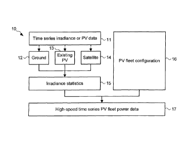
FIGURE 1 is a flow diagram showing a computer-implemented method for
estimating
power data for a photovoltaic power generation fleet in accordance with one
embodiment.
- 5 -
CA 02842932 2014-01-23
WO 2013/015851
PCT/US2012/032623
FIGURE 2 is a block diagram showing a computer-implemented system for
estimating
power data for a photovoltaic power generation fleet in accordance with one
embodiment.
FIGURE 3 is a graph depicting, by way of example, ten hours of time series
irradiance
data collected from a ground-based weather station with 10-second resolution.
FIGURE 4 is a graph depicting, by way of example, the clearness index that
corresponds
to the irradiance data presented in FIGURE 3.
FIGURE 5 is a graph depicting, by way of example, the change in clearness
index that
corresponds to the clearness index presented in FIGURE 4.
FIGURE 6 is a graph depicting, by way of example, the irradiance statistics
that
correspond to the clearness index in FIGURE 4 and the change in clearness
index in FIGURE 5.
FIGURES 7A-7B are photographs showing, by way of example, the locations of the
Cordelia Junction and Napa high density weather monitoring stations.
FIGURES 8A-8B are graphs depicting, by way of example, the adjustment factors
plotted
for time intervals from 10 seconds to 300 seconds.
FIGURES 9A-9F are graphs depicting, by way of example, the measured and
predicted
weighted average correlation coefficients for each pair of locations versus
distance.
FIGURES 10A-10F are graphs depicting, by way of example, the same information
as
depicted in FIGURES 9A-9F versus temporal distance.
FIGURES 11A-11F are graphs depicting, by way of example, the predicted versus
the
measured variances of clearness indexes using different reference time
intervals.
FIGURES 12A-12F are graphs depicting, by way of example, the predicted versus
the
measured variances of change in clearness indexes using different reference
time intervals.
FIGURES 13A-13F are graphs and a diagram depicting, by way of example,
application
of the methodology described herein to the Napa network.
FIGURE 14 is a graph depicting, by way of example, an actual probability
distribution
for a given distance between two pairs of locations, as calculated for a 1,000
meter x 1,000 meter
grid in one square meter increments.
FIGURE 15 is a graph depicting, by way of example, a matching of the resulting
model
to an actual distribution.
FIGURE 16 is a graph depicting, by way of example, results generated by
application of
Equation (65).
FIGURE 17 is a graph depicting, by way of example, the probability density
function
when regions are spaced by zero to five regions.
FIGURE 18 is a graph depicting, by way of example, results by application of
the model.
- 6 -
CA 02842932 2014-01-23
WO 2013/015851
PCT/US2012/032623
BEST MODE FOR CARRYING OUT THE INVENTION
Photovoltaic cells employ semiconductors exhibiting a photovoltaic effect to
generate
direct current electricity through conversion of solar irradiance. Within each
photovoltaic cell,
light photons excite electrons in the semiconductors to create a higher state
of energy, which acts
as a charge carrier for electric current. A photovoltaic system uses one or
more photovoltaic
panels that are linked into an array to convert sunlight into electricity. In
turn, a collection of
photovoltaic systems can be collectively operated as a photovoltaic fleet when
integrated into a
power grid, although the constituent photovoltaic systems may actually be
deployed at different
physical locations within a geographic region.
To aid with the planning and operation of photovoltaic fleets, whether at the
power grid,
supplemental, or standalone power generation levels, high resolution time
series of power output
data is needed to efficiently estimate photovoltaic fleet power production.
The variability of
photovoltaic fleet power generation under cloudy conditions can be efficiently
estimated, even in
the absence of high speed time series power production data, by applying a
fully derived
statistical approach. FIGURE 1 is a flow diagram showing a computer-
implemented method 10
for estimating power data for a photovoltaic power generation fleet in
accordance with one
embodiment. The method 10 can be implemented in software and execution of the
software can
be performed on a computer system, such as further described infra, as a
series of process or
method modules or steps.
Preliminarily, a time series of solar irradiance data is obtained (step 11)
for a set of
locations representative of the geographic region within which the
photovoltaic fleet is located or
intended to operate, as further described infra with reference to FIGURE 3.
Each time series
contains solar irradiance observations electronically recorded at known input
time intervals over
successive time periods. The solar irradiance observations can include
irradiance measured by a
representative set of ground-based weather stations (step 12), existing
photovoltaic systems (step
13), satellite observations (step 14), or some combination thereof. Other
sources of the solar
irradiance data are possible.
Next, the solar irradiance data in the time series is converted over each of
the time
periods, such as at half-hour intervals, into a set of clearness indexes,
which are calculated
relative to clear sky global horizontal irradiance. The set of clearness
indexes are interpreted into
as irradiance statistics (step 15), as further described infra with reference
to FIGURE 4-6. The
irradiance statistics for each of the locations is combined into fleet
irradiance statistics applicable
over the geographic region of the photovoltaic fleet. A time lag correlation
coefficient for an
- 7 -
CA 02842932 2015-10-01
WO 2013/015851 PC171.S21112/032623
output time interval is also determined to enable the generation of an output
time series at any
time resolution, even faster than the input data collection rate.
Finally, power statistics, including a time series of the power statistics for
the
photovoltaic fleet, are generated (step 17) as a function of the fleet
irradiance statistics and
system configuration, particularly the geographic distribution and power
rating of the
photovoltaic systems in the fleet (step 16). The resultant high-speed time
series fleet
performance data can be used to predictably estimate power output and
photovoltaic fleet
variability by fleet planners and operators, as well as other interested
parties.
The calculated irradiance statistics are combined with the photovoltaic fleet
configuration
to generate the high-speed time series photovoltaic production data. In a
further embodiment,
the foregoing methodology can be may also require conversion of weather data
for a region, such
as data from satellite regions, to average point weather data. A non-optimized
approach would
be to calculate a correlation coefficient matrix on-the-fly for each satellite
data point.
Alternatively, a conversion factor for performing area-to-point conversion of
satellite imagery
data is described in commonly-assigned U.S. Patent application, entitled
"Computer-
Implemented System and Method for Efficiently Performing Area-To-Point
Conversion of
Satellite Imagery for Photovoltaic Power Generation Fleet Output Estimation,"
Serial No.
13/190,449, filed July 25, 2011, pending.
The high resolution time series of power output data is determined in the
context of a
photovoltaic fleet, whether for an operational fleet deployed in the field, by
planners considering
fleet configuration and operation, or by other individuals interested in
photovoltaic fleet
variability and prediction. FIGURE 2 is a block diagram showing a computer-
implemented
system 20 fbr estimating power data for a photovoltaic power generation fleet
in accordance with
one embodiment. Time series power output data for a photovoltaic fleet is
generated using
observed field conditions relating to overhead sky clearness. Solar irradiance
23 relative to
prevailing cloudy conditions 22 in a geographic region of interest is
measured. Direct solar
irradiance measurements can be collected by ground-based weather stations 24.
Solar irradiance
measurements can also be inferred by the actual power output of existing
photovoltaic systems
25. Additionally, satellite observations 26 can be obtained for the geographic
region. Both the
direct and inferred solar irradiance measurements are considered to be sets of
point values that
relate to a specific physical location, whereas satellite imagery data is
considered to be a set of
area values that need to be converted into point values, as further described
infra. Still other
sources of solar irradiance measurements are possible.
- 8 -
CA 02842932 2014-01-23
WO 2013/015851
PCT/US2012/032623
The solar irradiance measurements are centrally collected by a computer system
21 or
equivalent computational device. The computer system 21 executes the
methodology described
supra with reference to FIGURE 1 and as further detailed herein to generate
time series power
data 26 and other analytics, which can be stored or provided 27 to planners,
operators, and other
parties for use in solar power generation 28 planning and operations. The data
feeds 29a-c from
the various sources of solar irradiance data need not be high speed
connections; rather, the solar
irradiance measurements can be obtained at an input data collection rate and
application of the
methodology described herein provides the generation of an output time series
at any time
resolution, even faster than the input time resolution. The computer system 21
includes
hardware components conventionally found in a general purpose programmable
computing
device, such as a central processing unit, memory, user interfacing means,
such as a keyboard,
mouse, and display, input/output ports, network interface, and non-volatile
storage, and execute
software programs structured into routines, functions, and modules for
execution on the various
systems. In addition, other configurations of computational resources, whether
provided as a
dedicated system or arranged in client-server or peer-to-peer topologies, and
including unitary or
distributed processing, communications, storage, and user interfacing, are
possible.
The detailed steps performed as part of the methodology described supra with
reference
to FIGURE 1 will now be described.
Obtain Time Series Irradiance Data
The first step is to obtain time series irradiance data from representative
locations. This
data can be obtained from ground-based weather stations, existing photovoltaic
systems, a
satellite network, or some combination sources, as well as from other sources.
The solar
irradiance data is collected from several sample locations across the
geographic region that
encompasses the photovoltaic fleet.
Direct irradiance data can be obtained by collecting weather data from ground-
based
monitoring systems. FIGURE 3 is a graph depicting, by way of example, ten
hours of time
series irradiance data collected from a ground-based weather station with 10-
second resolution,
that is, the time interval equals ten seconds. In the graph, the blue line 32
is the measured
horizontal irradiance and the black line 31 is the calculated clear sky
horizontal irradiance for the
location of the weather station.
Irradiance data can also be inferred from select photovoltaic systems using
their electrical
power output measurements. A performance model for each photovoltaic system is
first
identified, and the input solar irradiance corresponding to the power output
is determined.
- 9 -
CA 02842932 2014-01-23
WO 2013/015851
PCT/US2012/032623
Finally, satellite-based irradiance data can also be used. As satellite
imagery data is
pixel-based, the data for the geographic region is provided as a set of
pixels, which span across
the region and encompassing the photovoltaic fleet.
Calculate Irradiance Statistics
The time series irradiance data for each location is then converted into time
series
clearness index data, which is then used to calculate irradiance statistics,
as described infra.
Clearness Index (Kt)
The clearness index (Kt) is calculated for each observation in the data set.
In the case of
an irradiance data set, the clearness index is determined by dividing the
measured global
horizontal irradiance by the clear sky global horizontal irradiance, may be
obtained from any of a
variety of analytical methods. FIGURE 4 is a graph depicting, by way of
example, the clearness
index that corresponds to the irradiance data presented in FIGURE 3.
Calculation of the
clearness index as described herein is also generally applicable to other
expressions of irradiance
and cloudy conditions, including global horizontal and direct normal
irradiance.
Change in Clearness Index (AKt )
The change in clearness index (A1Ct ) over a time increment of At is the
difference
between the clearness index starting at the beginning of a time increment t
and the clearness
index starting at the beginning of a time increment t, plus a time increment
At. FIGURE 5 is a
graph depicting, by way of example, the change in clearness index that
corresponds to the
clearness index presented in FIGURE 4.
Time Period
The time series data set is next divided into time periods, for instance, from
five to sixty
minutes, over which statistical calculations are performed. The determination
of time period is
selected depending upon the end use of the power output data and the time
resolution of the input
data. For example, if fleet variability statistics are to be used to schedule
regulation reserves on a
30-minute basis, the time period could be selected as 30 minutes. The time
period must be long
enough to contain a sufficient number of sample observations, as defined by
the data time
interval, yet be short enough to be usable in the application of interest. An
empirical
investigation may be required to determine the optimal time period as
appropriate.
- 10 -
CA 02842932 2014-01-23
WO 2013/015851
PCT/US2012/032623
Fundamental Statistics
Table 1 lists the irradiance statistics calculated from time series data for
each time period
at each location in the geographic region. Note that time period and location
subscripts are not
included for each statistic for purposes of notational simplicity.
Statistic Variable
Mean clearness index P K1
Variance clearness index õv2
K1
Mean clearness index change
PAKt
Variance clearness index change ,2
1- AKt
Table!.
Table 2 lists sample clearness index time series data and associated
irradiance statistics
over five-minute time periods. The data is based on time series clearness
index data that has a
one-minute time interval. The analysis was performed over a five-minute time
period. Note that
the clearness index at 12:06 is only used to calculate the clearness index
change and not to
calculate the irradiance statistics.
Clearness Index (Kt) Clearness Index Change (AKt)
12:00 50% 40%
12:01 90% 0%
12:02 90% -80%
12:03 10% 0%
12:04 10% 80%
12:05 90% -40%
12:06 50%
Mean (it) 57% 0%
Variance (a) 13% 27%
Table 2.
The mean clearness index change equals the first clearness index in the
succeeding time
period, minus the first clearness index in the current time period divided by
the number of time
intervals in the time period. The mean clearness index change equals zero when
these two
values are the same. The mean is small when there are a sufficient number of
time intervals.
- 11 -
CA 02842932 2014-01-23
WO 2013/015851 PCT/US2012/032623
Furthermore, the mean is small relative to the clearness index change
variance. To simplify the
analysis, the mean clearness index change is assumed to equal zero for all
time periods.
FIGURE 6 is a graph depicting, by way of example, the irradiance statistics
that
correspond to the clearness index in FIGURE 4 and the change in clearness
index in FIGURE 5
using a half-hour hour time period. Note that FIGURE 6 presents the standard
deviations,
determined as the square root of the variance, rather than the variances, to
present the standard
deviations in terms that are comparable to the mean.
Calculate Fleet Irradiance Statistics
Irradiance statistics were calculated in the previous section for the data
stream at each
sample location in the geographic region. The meaning of these statistics,
however, depends
upon the data source. Irradiance statistics calculated from a ground-based
weather station data
represent results for a specific geographical location as point statistics.
Irradiance statistics
calculated from satellite data represent results for a region as area
statistics. For example, if a
satellite pixel corresponds to a one square kilometer grid, then the results
represent the irradiance
statistics across a physical area one kilometer square.
Average irradiance statistics across the photovoltaic fleet region are a
critical part of the
methodology described herein. This section presents the steps to combine the
statistical results
for individual locations and calculate average irradiance statistics for the
region as a whole. The
steps differs depending upon whether point statistics or area statistics are
used.
Irradiance statistics derived from ground-based sources simply need to be
averaged to
form the average irradiance statistics across the photovoltaic fleet region.
Irradiance statistics
from satellite sources are first converted from irradiance statistics for an
area into irradiance
statistics for an average point within the pixel. The average point statistics
are then averaged
across all satellite pixels to determine the average across the photovoltaic
fleet region.
Mean Clearness Index (/'Kt) and Mean Change in Clearness Index (uAKt )
The mean clearness index should be averaged no matter what input data source
is used,
whether ground, satellite, or photovoltaic system originated data. If there
are N locations, then
the average clearness index across the photovoltaic fleet region is calculated
as follows.
N ill Kt
ill N
Kt= E (1)
i=1
The mean change in clearness index for any period is assumed to be zero. As a
result, the
mean change in clearness index for the region is also zero.
- 12 -
CA 02842932 2014-01-23
WO 2013/015851
PCT/US2012/032623
AKt = (2)
Convert Area Variance to Point Variance
The following calculations are required if satellite data is used as the
source of irradiance
data. Satellite observations represent values averaged across the area of the
pixel, rather than
single point observations. The clearness index derived from this data (Kt
Area) may therefore be
considered an average of many individual point measurements.
N
Kt1
Kt Area = E
o)
N
As a result, the variance of the clearness index based on satellite data can
be expressed as
the variance of the average clearness index across all locations within the
satellite pixel.
N t
0 "K2 t_Are, =VAR[Kt Area ]=VAR K (4)
,.1 N
The variance of a sum, however, equals the sum of the covariance matrix.
N N
(72
Kt¨Area = ___________ 2 COV[Ktl , Kt ]
(5)
1=1 1=1
Let Kti
et p , represents the correlation coefficient between the
clearness index at
location i and location j within the satellite pixel. By definition of
correlation coefficient,
COV[Kti , Kt ]= t j Kt' p ' . Furthermore, since the objective is to
determine the
average point variance across the satellite pixel, the standard deviation at
any point within the
satellite pixel can be assumed to be the same and equals 0-Ki , which means
thatclic/al., =0"Zi
2 Kt' Kt
for all location pairs. As a result, CO V [Kt1 , Kt i= a Kt P ' .
Substituting this result into
Equation (5) and simplify.
( N N ,
2 2Ki',Kt
aKt- Area = aKt 2 L. (6)
N )/=1j=1
Suppose that data was available to calculate the correlation coefficient in
Equation (6).
The computational effort required to perform a double summation for many
points can be quite
large and computationally resource intensive. For example, a satellite pixel
representing a one
square kilometer area contains one million square meter increments. With one
million
increments, Equation (6) would require one trillion calculations to compute.
- 13 -
CA 02842932 2014-01-23
WO 2013/015851
PCT/US2012/032623
The calculation can be simplified by conversion into a continuous probability
density
function of distances between location pairs across the pixel and the
correlation coefficient for
that given distance, as further described supra. Thus, the irradiance
statistics for a specific
satellite pixel, that is, an area statistic, rather than a point statistics,
can be converted into the
irradiance statistics at an average point within that pixel by dividing by a
"Area" term (A) , which
corresponds to the area of the satellite pixel. Furthermore, the probability
density function and
correlation coefficient functions are generally assumed to be the same for all
pixels within the
fleet region, making the value of A constant for all pixels and reducing the
computational burden
further. Details as to how to calculate A are also further described supra.
2
2 Cr Kt - Area
a Kt SatellitePael (7)
AK1
where:
"N N
A Sale//lie Pixel Ez pi j
'Kt(8)
N2 ii=1 j=1
Likewise, the change in clearness index variance across the satellite region
can also be
converted to an average point estimate using a similar conversion factor,
AAAketa .
CY
õ 2
2 " AKt- Area
A v
ellitePixel (9)
AsAk
2 2
Variance of Clearness Index (a-ii ) and Variance of Change in Clearness Index
( crAKI )
At this point, the point statistics (o-K2, and c4,) have been determined for
each of several
representative locations within the fleet region. These values may have been
obtained from
either ground-based point data or by converting satellite data from area into
point statistics. If
the fleet region is small, the variances calculated at each location i can be
averaged to determine
the average point variance across the fleet region. If there are N locations,
then average variance
of the clearness index across the photovoltaic fleet region is calculated as
follows.
N
2 0-2
=
a Kt (10)
i=1 N
Likewise, the variance of the clearness index change is calculated as follows.
2
N 0
2 = ___________________
AKt N
(11)
i=1
- 14 -
CA 02842932 2014-01-23
WO 2013/015851
PCT/US2012/032623
Calculate Fleet Power Statistics
The next step is to calculate photovoltaic fleet power statistics using the
fleet irradiance
statistics, as determined supra, and physical photovoltaic fleet configuration
data. These fleet
power statistics are derived from the irradiance statistics and have the same
time period.
The critical photovoltaic fleet performance statistics that are of interest
are the mean fleet
power, the variance of the fleet power, and the variance of the change in
fleet power over the
desired time period. As in the case of irradiance statistics, the mean change
in fleet power is
assumed to be zero.
Photovoltaic System Power for Single System at Time t
Photovoltaic system power output (kW) is approximately linearly related to the
AC-
rating of the photovoltaic system (R in units of kWAc) times plane-of-array
irradiance. Plane-of-
array irradiance can be represented by the clearness index over the
photovoltaic system (KtPV)
times the clear sky global horizontal irradiance times an orientation factor
(0), which both
converts global horizontal irradiance to plane-of-array irradiance and has an
embedded factor
that converts irradiance from Watts/m2 to kW output/kW of rating. Thus, at a
specific point in
time (t), the power output for a single photovoltaic system (n) equals:
Pt" = Rn 0 in KtPV t" pear ,n
(12)
The change in power equals the difference in power at two different points in
time.
= Rn 0 tn+At KtPlitil+At tC+1Aecitr'n ¨ Rn Ktpv-rn tClear,n
(13)
The rating is constant, and over a short time interval, the two clear sky
plane-of-array
cln ,
irradiances are approximately the same ( rClear ,n rin r Clearn Ut-FAti
t+At t.ft t ), so that the three terms can
be factored out and the change in the clearness index remains.
A-Ptn At
7 tClear,n AKtp vin
(14)
Time Series Photovoltaic Power for Single System
I)" is a random variable that summarizes the power for a single photovoltaic
system n
over a set of times for a given time interval and set of time periods. AP n is
a random variable
that summarizes the change in power over the same set of times.
Mean Fleet Power (PP)
The mean power for the fleet of photovoltaic systems over the time period
equals the
expected value of the sum of the power output from all of the photovoltaic
systems in the fleet.
- 15-
CA 02842932 2014-01-23
WO 2013/015851
PCT/US2012/032623
p = E ERn On KtPVn 'Clear ,n (15)
_n=1
If the time period is short and the region small, the clear sky irradiance
does not change
much and can be factored out of the expectation.
(16)
/UP =PickarE ERnOnKtPVn
_n=1
Again, if the time period is short and the region small, the clearness index
can be
averaged across the photovoltaic fleet region and any given orientation factor
can be assumed to
be a constant within the time period. The result is that:
djD A .Fleet
etIP ii-t
(17)/Clear
where .1-// Clear is calculated, p¨ is taken from Equation (1) and:
Kt
RAdj.Fleet Rn on (18)
n=1
This value can also be expressed as the average power during clear sky
conditions times
the average clearness index across the region.
(19)
,Up = pClear ¨
Kt
2
Variance of Fleet Power ( CP )
The variance of the power from the photovoltaic fleet equals:
=VAR E Rn On KtP V n iClear,n (20)
_n=1
If the clear sky irradiance is the same for all systems, which will be the
case when the
region is small and the time period is short, then:
= VAR ICMar Rn On KtPV n (21)
n=1
The variance of a product of two independent random variables X, Y, that is,
VAR[XY])
equals EM2VAR[Y] + E[1]2VAR[X] + VAR[X]VAR[Y]. If the X random variable has a
large
mean and small variance relative to the other terms, then VAR[X* *12 VAR[Y].
Thus, the
clear sky irradiance can be factored out of Equation (21) and can be written
as:
-16-
CA 02842932 2014-01-23
WO 2013/015851
PCT/US2012/032623
f
P = iClear)2 VAR ERnKtPV"On (22)
_n=1
The variance of a sum equals the sum of the covariance matrix.
NN
2 (23)
cfP ( iClear)2 EECOV[RiKtPViOl,RiKtPriOjj
j=1
In addition, over a short time period, the factor to convert from clear sky
GHI to clear sky
POA does not vary much and becomes a constant. All four variables can be
factored out of the
covariance equation.
N N
(24)
p = kfr icrear)2 (R1 01)(RJ Of )COV[KtPV1 ,KtPV-1]
irljr4
For any i and j,= 2
COVIDP V ,KtPri 1/0"2 pKtiKt.;
= KtPV- KtPV-1 =
I NN
UP
p Kt' ,Kt
(25)
2 r =V-iickar )2 EE(Ri0')(Rial)11
Ktpvja K2 tpvj
0=1 j=1
As discussed supra, the variance of the satellite data required a conversion
from the
satellite area, that is, the area covered by a pixel, to an average point
within the satellite area. In
the same way, assuming a uniform clearness index across the region of the
photovoltaic plant,
the variance of the clearness index across a region the size of the
photovoltaic plant within the
fleet also needs to be adjusted. The same approach that was used to adjust the
satellite clearness
index can be used to adjust the photovoltaic clearness index. Thus, each
variance needs to be
adjusted to reflect the area that the ith photovoltaic plant covers.
2 _Ai 2
aKtPr Kt 0"--ki (26)
Substituting and then factoring the clearness index variance given the
assumption that the
average variance is constant across the region yields:
2 _ Adj.Fleet, , D Kt
(27)
P 1-4 'Clear I Kt
where the correlation matrix equals:
E
p Kt (Rjoi4,)(RiojAL)Kti KtP (28)
(E1=1 J=1
N Rn otty
n=1
R Adj.Fleet
'Clear in Equation (27) can be written as the power produced by the
photovoltaic fleet under clear sky conditions, that is:
-17-
CA 02842932 2014-01-23
WO 2013/015851
PCT/US2012/032623
2 CrP
pClear2 Kt 2
(29) =P
Kt
If the region is large and the clearness index mean or variances vary
substantially across
the region, then the simplifications may not be able to be applied.
Notwithstanding, if the
simplification is inapplicable, the systems are likely located far enough away
from each other, so
as to be independent. In that case, the correlation coefficients between
plants in different regions
would be zero, so most of the terms in the summation are also zero and an
inter-regional
simplification can be made. The variance and mean then become the weighted
average values
based on regional photovoltaic capacity and orientation.
Discussion
In Equation (28), the correlation matrix term embeds the effect of intra-plant
and inter-
plant geographic diversification. The area-related terms (A) inside the
summations reflect the
intra-plant power smoothing that takes place in a large plant and may be
calculated using the
simplified relationship, as further discussed supra. These terms are then
weighted by the
effective plant output at the time, that is, the rating adjusted for
orientation. The multiplication
of these terms with the correlation coefficients reflects the inter-plant
smoothing due to the
separation of photovoltaic systems from one another.
.2
Variance of Change in Fleet Power (0)
A similar approach can be used to show that the variance of the change in
power equals:
2 p A/Ct __
u AKt (30) AP =
1-1 Clear2
where:
N N Z.
p AKt Di ni Ai N(D infAi )pAKti (31)
= kJ. õ
., E J-1
(zN 1R n on )2
n=
The determination of Equations (30) and (31) becomes computationally intensive
as the
network of points becomes large. For example, a network with 10,000
photovoltaic systems
would require the computation of a correlation coefficient matrix with 100
million calculations.
The computational burden can be reduced in two ways. First, many of the terms
in the matrix
are zero because the photovoltaic systems are located too far away from each
other. Thus, the
double summation portion of the calculation can be simplified to eliminate
zero values based on
distance between locations by construction of a grid of points. Second, once
the simplification
-18-
CA 02842932 2014-01-23
WO 2013/015851 PCT/US2012/032623
has been made, rather than calculating the matrix on-the-fly for every time
period, the matrix can
be calculated once at the beginning of the analysis for a variety of cloud
speed conditions, and
then the analysis would simply require a lookup of the appropriate value.
Time Lag Correlation Coefficient
The next step is to adjust the photovoltaic fleet power statistics from the
input time
interval to the desired output time interval. For example, the time series
data may have been
collected and stored every 60 seconds. The user of the results, however, may
want to have
photovoltaic fleet power statistics at a 10-second rate. This adjustment is
made using the time
lag correlation coefficient.
The time lag correlation coefficient reflects the relationship between fleet
power and that
same fleet power starting one time interval (40 later. Specifically, the time
lag correlation
coefficient is defined as follows:
p,pAt COVIP,PAti
P = (32)
pu pAt
The assumption that the mean clearness index change equals zero implies that
2 2
Up& = Cr p . Given a non-zero variance of power, this assumption can also be
used to show that
COV[P, pA /1
=1Ap2 __ . Therefore:
2 262
P
2
P P 1 OPA
P =1 (33)
20-1.
This relationship illustrates how the time lag correlation coefficient for the
time interval
associated with the data collection rate is completely defined in terms of
fleet power statistics
already calculated. A more detailed derivation is described infra.
Equation (33) can be stated completely in terms of the photovoltaic fleet
configuration
and the fleet region clearness index statistics by substituting Equations (29)
and (30).
Specifically, the time lag correlation coefficient can be stated entirely in
terms of photovoltaic
fleet configuration, the variance of the clearness index, and the variance of
the change in the
clearness index associated with the time increment of the input data.
p AKt
P,PAl =.1 " AKt
(34)
2 p Kt
" Kt
- 19 -
CA 02842932 2014-01-23
WO 2013/015851
PCT/US2012/032623
Generate High-Speed Time Series Photovoltaic Fleet Power
The final step is to generate high-speed time series photovoltaic fleet power
data based on
irradiance statistics, photovoltaic fleet configuration, and the time lag
correlation coefficient.
This step is to construct time series photovoltaic fleet production from
statistical measures over
the desired time period, for instance, at half-hour output intervals.
A joint probability distribution function is required for this step. The
bivariate
probability density function of two unit normal random variables (X and Y)
with a correlation
coefficient of p equals:
1
y)= ___________________ exp (x2 +y2 ¨2pxy)
241- p2 _ 2(1¨P2) _ (35)
The single variable probability density function for a unit normal random
variable X
1 ( x2
1 0xalone is f(x)= __ e p ¨ ¨ . In addition, a conditional distribution for y
can be calculated
V2n- 2
based on a known x by dividing the bivariate probability density function by
the single variable
probability density (i.e., f (Ylx)= f (x' ). Making the appropriate
substitutions, the result is that
f (x)
the conditional distribution of y based on a known x equals:
1 (Y ¨ Px)2 -
_________________________ exp
-shr; p2 _ 2(1¨P2) (36)
Ypx
Define a random variable Z = , -and substitute into Equation (36). The result
is
111¨ p2
that the conditional probability of z given a known x equals:
f(zix)= ,-- exp( z2
V271- 2 (37)
The cumulative distribution function for Z can be denoted by 0(z* ) , where z*
represents a specific value for z. The result equals a probability (p) that
ranges between 0 (when
z = ¨ ) and 1 (when z =00 ). The function represents the cumulative
probability that any
value of z is less than z* , as determined by a computer program or value
lookup.
1jrz*
P= exp(--z2)dz f
0(z*)= ___________________________________________________________ (38)
2
Rather than selecting z* , however, a probability p falling between 0 and 1
can be
selected and the corresponding z* that results in this probability found,
which can be
accomplished by taking the inverse of the cumulative distribution function.
-20 -
CA 02842932 2014-01-23
WO 2013/015851 PCT/US2012/032623
0-I(P)=z* (39)
Substituting back for z as defined above results in:
p2 (40)
D At ,,
FipA
P
Now, let the random variables equal x= __________ and with the
apA
correlation coefficient being the time lag correlation coefficient between P
and PAt(i.e., let
p At
P= P ). When At is small, then the mean and standard deviations for
P' are
approximately equal to the mean and standard deviation for P. Thus, Y can be
restated as
p At
Y ___________
. Add a time subscript to all of the relevant data to represent a specific
point in
o-p
time and substitute x, y, and p into Equation (40).
r P At t ,t/p P,PA1 Pt ¨11p
P) o-
P
\
(41)
Vi_pP,PA /2
The random variable kir, however, is simply the random variable P shifted in
time by a
time interval of At. As a result, at any given time t, PAtt =P1+ At . Make
this substitution into
Equation (41) and solve in terms of Pt+ At .
At nAt At2
PH-At PP 'P Pt +(1¨ PF )Pp-F\10-p2 (1¨ P`DioD '` )0 i(P)
(42)
At any given time, photovoltaic fleet power equals photovoltaic fleet power
under clear
sky conditions times the average regional clearness index, that is, Pt = pick"
Kt,. In addition,
2 n
over a short time period, ,up "=,' PtClearit (rClear
z and up t P Kt c4. Substitute these
three
relationships into Equation (42) and factor out photovoltaic fleet power under
clear sky
conditions (Clear ).
) as common to all three terms.
PPAI
P Kt t + - p"A`),u- +
Kt
p= pClear .\ _________________________
ti-At t Az \ (43)
/
pKt cr2 1_ pP ,P
0¨ 1 (Pt)
Kt
- 21 -
CA 02842932 2015-10-01
WO 2013/015851
PCT/US2012/032623
Equation (43) provides an iterative method to generate high-speed time series
photovoltaic production data for a fleet of photovoltaic systems. At each time
step (1-1-41), the
power delivered by the fleet of photovoltaic systems ( PI+At ) is calculated
using input values
from time step/. Thus, a time series of power outputs can be created. The
inputs include:
p Clear
= I ¨
photovoltaic fleet power during clear sky conditions calculated using a
photovoltaic simulation program and clear sky irradiance.
= 11 ¨average regional clearness index inferred based on Pt calculated in
time step t,
Kit -brat
that is,
= Kt ¨mean clearness index calculated using time series irradiance data and
Equation (1).
2
a--
= Ks ¨ variance of the clearness index calculated using time series
irradiance data and
Equation (10).
p,pAl
= ¨ fleet configuration as reflected in the time lag correlation
coefficient
calculated using Equation (34). In turn, Equation (34), relies upon
correlation
coefficients from Equations (28) and (31). A method to obtain these
correlation
coefficients by empirical means is described in commonly-assigned U.S. Patent
application, entitled "Computer-Implemented System and Method for Determining
Point-To-Point Correlation Of Sky Clearness for Photovoltaic Power Generation
Fleet Output Estimation," Serial No. 13/190,435, filed July 25, 2011, pending,
and
U.S. Patent application, entitled "Computer-Implemented System and Method for
Efficiently Performing Area-To-Point Conversion of Satellite Imagery for
Photovoltaic Power Generation Fleet Output Estimation," Serial No. 13/190,449,
filed July 25, 2011, pending.
= r" ri,
fleet configuration as reflected in the clearness index correlation
coefficient
matrix calculated using Equation (28) where, again, the correlation
coefficients may
be obtained using the empirical results as further described infra.
= Cf.' (Pt) ¨ the inverse cumulative normal distribution function based on
a random
variable between 0 and 1.
- 22 -
CA 02842932 2014-01-23
WO 2013/015851
PCT/US2012/032623
Derivation of Empirical Models
The previous section developed the mathematical relationships used to
calculate
irradiance and power statistics for the region associated with a photovoltaic
fleet. The
relationships between Equations (8), (28), (31), and (34) depend upon the
ability to obtain point-
to-point correlation coefficients. This section presents empirically-derived
models that can be
used to determine the value of the coefficients for this purpose.
A mobile network of 25 weather monitoring devices was deployed in a 400 meter
by 400
meter grid in Cordelia Junction, CA, between November 6, 2010, and November
15, 2010, and
in a 4,000 meter by 4,000 meter grid in Napa, CA, between November 19, 2010,
and November
24, 2010. FIGURES 7A-7B are photographs showing, by way of example, the
locations of the
Cordelia Junction and Napa high density weather monitoring stations.
An analysis was performed by examining results from Napa and Cordelia Junction
using
10, 30, 60, 120 and 180 second time intervals over each half-hour time period
in the data set.
The variance of the clearness index and the variance of the change in
clearness index were
calculated for each of the 25 locations for each of the two networks. In
addition, the clearness
index correlation coefficient and the change in clearness index correlation
coefficient for each of
the 625 possible pairs, 300 of which are unique, for each of the two locations
were calculated.
An empirical model is proposed as part of the methodology described herein to
estimate
the correlation coefficient of the clearness index and change in clearness
index between any two
points by using as inputs the following: distance between the two points,
cloud speed, and time
interval. For the analysis, distances were measured, cloud speed was implied,
and a time interval
was selected.
The empirical models infra describe correlation coefficients between two
points (i and j),
making use of "temporal distance," defined as the physical distance (meters)
between points i
and j, divided by the regional cloud speed (meters per second) and having
units of seconds. The
temporal distance answers the question, "How much time is needed to span two
locations?"
Cloud speed was estimated to be six meters per second. Results indicate that
the
clearness index correlation coefficient between the two locations closely
matches the estimated
value as calculated using the following empirical model:
\ClearnessPower
pK =exp(Ci x TemporalDistance) (44)
where TemporalDistance = Distance (meters) / CloudSpeed (meters per second),
Clearness Power = In (C2At )-- k , such that 5 < k< 15, where the expected
value is k= 9.3,
At is the desired output time interval (seconds), and C1= 10-3 seconds-1, and
C2 = 1 seconds'.
- 23 -
CA 02842932 2014-01-23
WO 2013/015851 PCT/US2012/032623
Results also indicate that the correlation coefficient for the change in
clearness index
between two locations closely matches the values calculated using the
following empirical
relationship:
AKti ,AKti K1 Kt-
ClearnessPower
t
fit (45)
Kt',Kt3 171
where P is calculated using Equation (44) and AClearnessP ower =1+
2 At , such
that 100 < m < 200, where the expected value is m = 140.
Empirical results also lead to the following models that may be used to
translate the
variance of clearness index and the variance of change in clearness index from
the measured
time interval ( At ref) to the desired output time interval ( At ).
I A
2 2
UK!, ay, exp 1
--At ref (46)
At ref
\c3_}
2 2
CYAK = CrAK 1 ¨ 2 1 At
Al t At ref (47)
At ref
where C3= 0.1 < C3 < 0.2, where the expected value is C3 = 0.15.
FIGURES 8A-8B are graphs depicting, by way of example, the adjustment factors
plotted
for time intervals from 10 seconds to 300 seconds. For example, if the
variance is calculated at a
300-second time interval and the user desires results at a 10-second time
interval, the adjustment
for the variance clearness index would be 1.49
These empirical models represent a valuable means to rapidly calculate
correlation
coefficients and translate time interval with readily-available information,
which avoids the use
of computation-intensive calculations and high-speed streams of data from many
point sources,
as would otherwise be required.
Validation
Equations (44) and (45) were validated by calculating the correlation
coefficients for
every pair of locations in the Cordelia Junction network and the Napa network
at half-hour time
periods. The correlation coefficients for each time period were then weighted
by the
corresponding variance of that location and time period to determine weighted
average
correlation coefficient for each location pair. The weighting was performed as
follows:
- 24 -
CA 02842932 2014-01-23
WO 2013/015851
PCT/US2012/032623
_______________________ vT 2 Kt' ,Kt
Kt' ,Kt L-di_-1 Cr Kt- ,,
:
P =T ,and
________________________ v T 2 ,A1Cti AKti
AKt` ,AKti ___________________________
P=
0.A2
1 Kt_i,
FIGURES 9A-9F are graphs depicting, by way of example, the measured and
predicted
weighted average correlation coefficients for each pair of locations versus
distance. FIGURES
10A-10F are graphs depicting, by way of example, the same information as
depicted in
FIGURES 9A-9F versus temporal distance, based on the assumption that cloud
speed was 6
meters per second. The upper line and dots appearing in close proximity to the
upper line
present the clearness index and the lower line and dots appearing in close
proximity to the lower
line present the change in clearness index for time intervals from 10 seconds
to 5 minutes. The
symbols are the measured results and the lines are the predicted results.
Several observations can be drawn based on the information provided by the
FIGURES
9A-9F and 10A-10F. First, for a given time interval, the correlation
coefficients for both the
clearness index and the change in the clearness index follow an exponential
decline pattern
versus distance (and temporal distance). Second, the predicted results are a
good representation
of the measured results for both the correlation coefficients and the
variances, even though the
results are for two separate networks that vary in size by a factor of 100.
Third, the change in the
clearness index correlation coefficient converges to the clearness correlation
coefficient as the
time interval increases. This convergence is predicted based on the form of
the empirical model
because AClearness Power approaches one as At becomes large.
Equation (46) and (47) were validated by calculating the average variance of
the
clearness index and the variance of the change in the clearness index across
the 25 locations in
each network for every half-hour time period. FIGURES 11A-11F are graphs
depicting, by way
of example, the predicted versus the measured variances of clearness indexes
using different
reference time intervals. FIGURES 12A-12F are graphs depicting, by way of
example, the
predicted versus the measured variances of change in clearness indexes using
different reference
time intervals. FIGURES 11A-11F and 12A-12F suggest that the predicted results
are similar to
the measured results.
Discussion
The point-to-point correlation coefficients calculated using the empirical
forms described
supra refer to the locations of specific photovoltaic power production sites.
Importantly, note
- 25 -
CA 02842932 2014-01-23
WO 2013/015851
PCT/US2012/032623
that the data used to calculate these coefficients was not obtained from time
sequence
measurements taken at the points themselves. Rather, the coefficients were
calculated from
fleet-level data (cloud speed), fixed fleet data (distances between points),
and user-specified data
(time interval).
The empirical relationships of the foregoing types of empirical relationships
may be used
to rapidly compute the coefficients that are then used in the fundamental
mathematical
relationships. The methodology does not require that these specific empirical
models be used
and improved models will become available in the future with additional data
and analysis.
Example
This section provides a complete illustration of how to apply the methodology
using data
from the Napa network of 25 irradiance sensors on November 21, 2010. In this
example, the
sensors served as proxies for an actual 1 kW photovoltaic fleet spread evenly
over the
geographical region as defined by the sensors. For comparison purposes, a
direct measurement
approach is used to determine the power of this fleet and the change in power,
which is
accomplished by adding up the 10-second output from each of the sensors and
normalizing the
output to a 1 kW system. FIGURES 13A-13F are graphs and a diagram depicting,
by way of
example, application of the methodology described herein to the Napa network.
The predicted behavior of the hypothetical photovoltaic fleet was separately
estimated
using the steps of the methodology described supra. The irradiance data was
measured using
ground-based sensors, although other sources of data could be used, including
from existing
photovoltaic systems or satellite imagery. As shown in FIGURE 13A, the data
was collected on
a day with highly variable clouds with one-minute global horizontal irradiance
data collected at
one of the 25 locations for the Napa network and specific 10-second measured
power output
represented by a blue line. This irradiance data was then converted from
global horizontal
irradiance to a clearness index. The mean clearness index, variance of
clearness index, and
variance of the change in clearness index was then calculated for every 15-
minute period in the
day. These calculations were performed for each of the 25 locations in the
network. Satellite-
based data or a statistically-significant subset of the ground measurement
locations could have
also served in place of the ground-based irradiance data. However, if the data
had been collected
from satellite regions, an additional translation from area statistics to
average point statistics
would have been required. The averaged irradiance statistics from Equations
(1), (10), and (11)
are shown in FIGURE 13B, where standard deviation (o) is presented, instead of
variance (a2) to
plot each of these values in the same units.
- 26 -
CA 02842932 2014-01-23
WO 2013/015851
PCT/US2012/032623
In this example, the irradiance statistics need to be translated since the
data were recorded
at a time interval of 60 seconds, but the desired results are at a 10-second
resolution. The
translation was performed using Equations (46) and (47) and the result is
presented in FIGURE
13C.
The details of the photovoltaic fleet configuration were then obtained. The
layout of the
fleet is presented in FIGURE 13D. The details include the location of the each
photovoltaic
system (latitude and longitude), photovoltaic system rating (1/25 kW), and
system orientation
(all are horizontal).
Equation (43), and its associated component equations, were used to generate
the time
series data for the photovoltaic fleet with the additional specification of
the specific empirical
models, as described in Equations (44) through (47). The resulting fleet power
and change in
power is presented represented by the red lines in FIGURES 12E and 12F.
Probability Density Function
The conversion from area statistics to point statistics relied upon two terms
AKt and
261AKt to calculate oj, and a , respectively. This section considers these
terms in more detail.
For simplicity, the methodology supra applies to both Kt and AKt, so this
notation is dropped.
Understand that the correlation coefficient pij could refer to either the
correlation coefficient for
clearness index or the correlation coefficient for the change in clearness
index, depending upon
context. Thus, the problem at hand is to evaluate the following relationship:
r _____________ 1 ji if j
(48)
The computational effort required to calculate the correlation coefficient
matrix can be
substantial. For example, suppose that the one wants to evaluate variance of
the sum of points
within a 1 square kilometer satellite region by breaking the region into one
million square meters
(1,000 meters by 1,000 meters). The complete calculation of this matrix
requires the
examination of 1 trillion (1012) location pair combinations.
Discrete Formulation
The calculation can be simplified using the observation that many of the terms
in the
correlation coefficient matrix are identical. For example, the covariance
between any of the one
million points and themselves is 1. This observation can be used to show that,
in the case of a
rectangular region that has dimension of H by W points (total of N) and the
capacity is equal
distributed across all parts of the region that:
- 27 -
CA 02842932 2014-01-23
WO 2013/015851
PCT/US2012/032623
2k [0 jApd
( 1 N N ( 1 \ H -1 i
v2 ZE Pl'i =
\ ¨ i=1 j=1 \ N2 I 2k KW APd (49)
i=0 j=0
where:
¨1, when i = 0 and j = 0
k= 1, when j = 0 or j = i
2, when 0 <j <i
When the region is a square, a further simplification can be made.
1 ri 2) z -11 -
(50)
(50)
where:
0, when i = 0 and j = 0
k = 2, when j = 0 or j = i ,and
3, when 0 <j < i
d=(vi2 __________ + J2 )(VArea
IN-1
The benefit of Equation (50) is that there are N rather than N2 unique
combinations
2
that need to be evaluated. In the example above, rather than requiring one
trillion possible
combinations, the calculation is reduced to one-half million possible
combinations.
Continuous Formulation
Even given this simplification, however, the problem is still computationally
daunting,
especially if the computation needs to be performed repeatedly in the time
series. Therefore, the
problem can be restated as a continuous formulation in which case a proposed
correlation
function may be used to simplify the calculation. The only variable that
changes in the
correlation coefficient between any of the location pairs is the distance
between the two
locations; all other variables are the same for a given calculation. As a
result, Equation (50) can
be interpreted as the combination of two factors: the probability density
function for a given
distance occurring and the correlation coefficient at the specific distance.
Consider the probability density function. The actual probability of a given
distance
between two pairs occurring was calculated for a 1,000 meter x 1,000 meter
grid in one square
meter increments. The evaluation of one trillion location pair combination
possibilities was
evaluated using Eauation (48) and by eliminating the correlation coefficient
from the equation.
- 28 -
CA 02842932 2014-01-23
WO 2013/015851
PCT/US2012/032623
FIGURE 14 is a graph depicting, by way of example, an actual probability
distribution for a
given distance between two pairs of locations, as calculated for a 1,000 meter
x 1,000 meter grid
in one square meter increments.
The probability distribution suggests that a continuous approach can be taken,
where the
goal is to find the probability density function based on the distance, such
that the integral of the
probability density function times the correlation coefficient function
equals:
A= f (D)p(d)dD
(51)
An analysis of the shape of the curve shown in FIGURE 14 suggests that the
distribution
can be approximated through the use of two probability density functions. The
first probability
density function is a quadratic function that is valid between 0 and ./
Area .
6
D ,D2 \ for 1:)._D Area
fQuad='(Area)\ NI Area (52)
0 for D> Area
This function is a probability density function because integrating between 0
andequals 1
Area
(i.e.,
r ¨ I A ea
13{13 "" D Ared¨ f Quaddp =1 ).
The second function is a normal distribution with a mean of -"Area and
standard
deviation of 0.1VArea
(
1 / D-11 Area \2
\
1 2 0.1*VArea
e _______________________________________________________________ (53)
f Norm = .1* AI Area ).µ127-c
Likewise, integrating across all values equals 1.
To construct the desired probability density function, take, for instance, 94
percent of the
quadratic density function plus 6 of the normal density function.
r+oo
f = 0 .9 4 .1 Area f Quad dD + 0.06 j_03 Norm di) (54)
FIGURE 15 is a graph depicting, by way of example, a matching of the resulting
model
to an actual distribution.
The result is that the correlation matrix of a square area with uniform point
distribution as
N gets large can be expressed as follows, first dropping the subscript on the
variance since this
equation will work for both Kt and AKt.
A 0.94 joAl Area f Quadp(D)C1D 0.06 f+c f p(D)c1D
Norm (55)
-29..
CA 02842932 2014-01-23
WO 2013/015851
PCT/US2012/032623
where p(D) is a function that expresses the correlation coefficient as a
function of
distance (D).
Area to Point Conversion Using Exponential Correlation Coefficient
Equation (55) simplifies the problem of calculating the correlation
coefficient and can be
implemented numerically once the correlation coefficient function is known.
This section
demonstrates how a closed form solution can be provided, if the functional
form of the
correlation coefficient function is exponential.
Noting the empirical results as shown in the graph in FIGURES 9A-9F, an
exponentially
decaying function can be taken as a suitable form for the correlation
coefficient function.
Assume that the functional form of correlation coefficient function equals:
x D
p(D)= e=%1 Area (56)
f NI Area
Quad p(D) dD
Let Quad be the solution to J
xi)
(D __
Quad= FloArea
f Qõad p(D)dD = D2 eVA"a dD (57)
Area) ,Area
Integrate to solve.
x D ( ( x D
\ 2
X
_______________________________________________ D + 2 e`l¨Area
x rATei;
Quad = (6) ( __________ D 1 e D2 ¨2 Alib¨va Area
Area (58)
Complete the result by evaluating at D equal to -"Area for the upper bound and
0 for the
lower bound. The result is:
( 6 \ r
Quad= ¨ [(x ¨ 2Xe + 1) + 4]
3
(59)
+ (D)dD
Next, consider the solution to -f_f
oo
Norm19 , which will be called Norm.
( +001)(D¨P)2 x D
Norm= r--1¨ e (2 Cr eV Area dij
(60)
O
Where-
p=,/
Area and 0 =0.1-1Area . Simplifying:
-30-
CA 02842932 2014-01-23
WO 2013/015851
PCT/US2012/032623
1 x 1 \
11
Norm= eV Area(+ (2 Al Area)
\CF
\-2
x 2
(1 (61)
2
D (Area,u+
) Al
. o-
+ c
= - dD
J
_____________________________ 2
D -F __
cy
Substitute zr. , -.I Area ) and o-dz=dD
____________________________ 1 x 0.2 ( _ 1 2,2
________________________ P
Norm= e-J Area (2 11 Area, ) 1 .1"" e(2) dz
(62)
1127-1.
Integrate and solve.
r (
X)
0.2 (63)
P+ _________________________
Norm= eAl Area 2 Area
Substitute the mean of -"Area and the standard deviation of o.i-JArea into
Equation (63).
Norm= ex0+ 0.0054
(64)
Substitute the solutions for Quad and Norm back into Equation (55). The result
is the
ratio of the area variance to the average point variance. This ratio was
referred to as A (with the
appropriate subscripts and superscripts) supra.
A=0.94(----kx-2)(ex +1)+4}+0.06ex(1+" 54 (65)
X3
Example
This section illustrates how to calculate A for the clearness index for a
satellite pixel that
covers a geographical surface area of 1 km by 1 km (total area of 1,000,000
m2), using a 60-
second time interval, and 6 meter per second cloud speed. Equation (56)
required that the
xD
correlation coefficient be of the form eV Area . The empirically derived
result in Equation (44)
can be rearranged and the appropriate substitutions made to show that the
correlation coefficient
of the clearness index equals exp- on At ¨9.3)D1. Multiply the exponent by
VArea so_ _
that the
woo CloudSpeed j 1 Area
-31 -
CA 02842932 2014-01-23
WO 2013/015851
PCT/US2012/032623
n ________________________________________ V e
correlation coefficient equals exp O At -9.3)Ara D
,
_____________________________________________________________________________
. This expression is now in the correct
1000 CloudSpeed Al Area
form to apply Equation (65), where x= On At -9.3)V Area . Inserting the
assumptions results in
moo CloudSpeed
On 60 - 9.3)V1,000,000
x- - 0.86761, which is applied to Equation (65). The result
is that A equals 65
1000x6
percent, that is, the variance of the clearness index of the satellite data
collected over a 1 km2
region corresponds to 65 percent of the variance when measured at a specific
point. A similar
approach can be used to show that the A equals 27 percent for the change in
clearness index.
FIGURE 16 is a graph depicting, by way of example, results generated by
application of
Equation (65).
Time Lag Correlation Coefficient
This section presents an alternative approach to deriving the time lag
correlation
coefficient. The variance of the sum of the change in the clearness index
equals:
2
CrE AKt = V AR[E(KtAt ¨ Kt (66)
where the summation is over N locations. This value and the corresponding
subscripts have been
excluded for purposes of notational simplicity.
Divide the summation into two parts and add several constants to the equation:
(67)
2 E Kt At
E Kt
o-E AKt =VAR o-E law aE Kt 0_
a KtAt Kt ,
_
Since cEKtaa 0Kt (or clE KtAi = cE Kt if the first term in Kt and the last
term in
Kt' are the same):
(68)
AKt
2 Kt At E Kt
E
tgE 0-2 VAR Kt
CIE Kt At CrE Kt
The variance term can be expanded as follows:
- 32 -
CA 02842932 2014-01-23
WO 2013/015851
PCT/US2012/032623
VAR E KtAti VAR[EKt] (69)
2 2
CrE Kt At CI Kt
rr 2 er, 2
`'EAKt =--"'E Kt 2COV L Kt E Kt At
E Kta Kt At
Since CO qEKt, EKtAt aK 0_ A, nõ,K,A,
E t E Kt V , the first two
terms equal
one and the covariance term is replaced by the correlation coefficient.
E
2 Kt ,E Kt At ) (70)
CrEAKt = 2o- Kt(1 ¨ p
This expression rearranges to:
( Z 2 Kt,EKtAt1 1 (TAD
(71)
=
2 0-2
Kt )
Assume that all photovoltaic plant ratings, orientations, and area adjustments
equal to
one, calculate statistics for the clearness alone using the equations
described supra and then
substitute. The result is:
EKt,EKIAt
=1 p AK/ 0.2
(72)
MCI
2P Ki
Kt
Relationship Between Time Lag Correlation Coefficient and Power/Change in
Power Correlation
Coefficient
This section derives the relationship between the time lag correlation
coefficient and the
correlation between the series and the change in the series for a single
location.
P COV [P, AP} = CO V , PAI -p1 COV[P,
P 01,
P
2 2
crpCTAp 1144AP al'dP
2
Since o-Ap = VAR[P At ¨ Pl= crp2 + 61
2 ¨ 2COVI.P , PAt j, and
p4
CO+ P
p2 At ,then:
- 33 -
CA 02842932 2014-01-23
WO 2013/015851
PCT/US2012/032623
P,P 1 V 2 2 2
CIP
PAP P '
P= __________________________________________
D DAI _______________________________________
1/013. (0-3 + a 2 -2licricr2 )
P ' p41
2 2
Since a p "-^-'' 0- pet , this expression can be further simplified. Then,
square both
expression and solve for the time lag correlation coefficient:
P,PA' =1- 2(p P'AP )2
P
Correlation Coefficients Between Two Regions
Assume that the two regions are squares of the same size, each side with N
points, that is,
a matrix with dimensions of VT/ by AfTv points, where ,17-v is an integer, but
are separated by
one or more regions. Thus:
-
2 (73) 2, 2,
,...._kk ` IN -iAlIN -1-11P-
i _ 1=0j=i-, i N
where:
1, when i = 0
k = ,and
2, when i >O
d= A1/2 4- () -1- ATM V IITI¨rea , and
such that M equals the number of regions.
FIGURE 17 is a graph depicting, by way of example, the probability density
function
when regions are spaced by zero to five regions. FIGURE 17 suggests that the
probability
density function can be estimated using the following distribution:
1-
f = 1+(Spacing- D\
-\ 1
Spacing- D
V
0 for Spacing- V Area Lc D ._._ Spacing
for Spacing 5_ D ._-_ Spacing + V Area
Area i
all else (74)
Area
This function is a probability density function because the integration over
all possible
values equals zero. FIGURE 18 is a graph depicting, by way of example, results
by application
of this model.
While the invention has been particularly shown and described as referenced to
the
embodiments thereof, those skilled in the art will understand that the
foregoing and other
changes in form and detail may be made therein without departing from the
spirit and scope.
- 34 -