Note: Descriptions are shown in the official language in which they were submitted.
CA 02853255 2014-05-30
DESIGNING A 3D MODELED OBJECT WITH 2D VIEWS
FIELD OF THE INVENTION
The invention relates to the field of computer programs and systems, and more
specifically to a method, system and program for designing a three-dimensional
modeled (3D) modeled object, as well as a 3D modeled object obtainable by said
method and a data file storing said 3D modeled object.
BACKGROUND
A number of systems and programs are offered on the market for the design,
the engineering and the manufacturing of objects. CAD is an acronym for
Computer-
Aided Design, e.g. it relates to software solutions for designing an object.
CAE is an
acronym for Computer-Aided Engineering, e.g. it relates to software solutions
for
simulating the physical behavior of a future product. CAM is an acronym for
Computer-Aided Manufacturing, e.g. it relates to software solutions for
defining
manufacturing processes and operations. In such systems, the graphical user
interface
(GUI) plays an important role as regards the efficiency of the technique.
These
techniques may be embedded within Product Lifecycle Management (PLM) systems.
PLM refers to a business strategy that helps companies to share product data,
apply
common processes, and leverage corporate knowledge for the development of
products from conception to the end of their life, across the concept of
extended
enterprise.
The PLM solutions provided by Dassault Systemes (under the trademarks
CATIA, ENOVIA and DELMIA) provide an Engineering Hub, which organizes
product engineering knowledge, a Manufacturing Hub, which manages
manufacturing engineering knowledge, and an Enterprise Hub which enables
enterprise integrations and connections into both the Engineering and
Manufacturing
Hubs. All together the system delivers an open object model linking products,
processes, resources to enable dynamic, knowledge-based product creation and
decision support that drives optimized product definition, manufacturing
preparation,
production and service.
Some CAD systems now allow the user to design a 3D modeled object based
on a set of two-dimensional (2D) pictures, for example photos, of a real
object that is
to be modeled. Existing methods include providing to the system several
overlapping
CA 02853255 2014-05-30
2
pictures representing the real object from different angles. Then, the user is
involved
to match up identical points, lines and edges across the pictures. Optionally,
the user
adds curves on pictures, while maintaining the overlapping coherence. The next
step
is for the system to automatically compute a 3D version of the object. The
geometry
of this object is a set of 3D points, curves and lines representing
characteristic edges.
It may be wireframe geometry. Optionally, the user adds 3D curves on this
wireframe geometry. The user is involved again to create surfaces bounded by
the
curves computed at previous steps. Boundary curves of each surface are
selected by
the user. Depending on the application, a wireframe model, a surface model or
even a
solid model might be created from the initial pictures, although this is not
perfectly
clear from prior art literature.
As can be seen, this prior art involves the user during two steps. The first
step
is to set up the matching across overlapping pictures. This step seems to be
unavoidable. After the system has created 3D curves, the other step is for the
user to
select boundary curves in order for the system to create surfaces. This manual
selection is required because the systems of the prior art are unable to
automatically
create surfaces from 3D curves. This manual process can be very long and
tedious
from the user point of view. Furthermore, an incorrect selection results in
twisted or
overlapping surfaces. Identifying and repairing these pathological surfaces is
the
user's responsibility, which lengthens again the path to the virtual 3D
object.
Thus, the invention aims at improving the design of 3D modeled objects based
on 2D views.
SUMMARY OF THE INVENTION
According to one aspect, it is therefore provided a computer-implemented
method for designing a three-dimensional modeled object. The method comprises
the
step of providing a plurality of two-dimensional views of the modeled object
having
curves and points defined thereon, a three-dimensional wireframe graph
comprising
edges that connect vertices, and correspondences between the edges and the
vertices
with respectively curves and points on the views. The method also comprises
the step
of associating, to each vertex of the wireframe graph, a local radial order
between all
the edges incident to the vertex, according to local partial radial orders
between the
curves corresponding to the edges on each of the views with respect to the
point
corresponding to the vertex. And then the method comprises the step of
determining
CA 02853255 2014-05-30
3
edge cycles, by browsing the wireframe graph following the local radial orders
associated to the vertices.
The method may comprise one or more of the following:
- wherein associating, to each vertex of the wireframe graph, a local radial
order between all the edges incident to a respective vertex comprises, for
each respective vertex, determining, for each view, the local partial radial
order with respect to the point corresponding to the respective vertex
between curves that are defined on the view and that correspond to an
edge incident to the respective vertex, merging all the local partial radial
orders, and traversing the result of the merging of all the local partial
radial orders to detect a cycle including all the edges incident to the
respective vertex, said cycle constituting the local radial order associated
to the respective vertex;
- the local partial radial orders are determined as graphs of which nodes
identify edges and of which arcs identify subsequence between edges;
- associating, to each vertex of the wireframe graph, a local radial order
between all the edges incident to a respective vertex further comprises,
when traversing the result of the merging of all the local partial radial
orders leads to detecting several cycles including all the edges incident to
the respective vertex, selecting one of the cycles detected for said
respective vertex, said respective vertex being a singular vertex;
- selecting one of the cycles detected comprises performing a
regularization process on the set of all singular vertices, the
regularization process comprising chosing a starting singular vertex and a
starting output edge of said starting singular vertex, browsing the
wireframe graph following the local radial orders associated to the
vertices to detect an edge cycle at said starting singular vertex, and then,
if reaching another singular vertex, repeating the regularization process
with a new starting singular vertex and/or a new starting output edge,
else, associating to said starting singular vertex the cycle, detected when
traversing the result of the merging of all the local partial radial orders
leads, that is compliant with the order between the starting output edge
and the final edge browsed, removing the starting singular vertex from
CA 02853255 2014-05-30
= 4
the set of all singular vertices, and then repeating the regularization
process until no singular vertex remains;
- determining edge cycles by browsing the wireframe graph comprises the
sub-steps of chosing a vertex, forming an edge list by following, starting
from the chosen vertex, the local radial orders associated to the vertices
as they are encountered, and incrementing the edge list with the followed
edges, until the edge list forms an edge cycle, and repeating the
preceding sub-steps;
- the views are images and the wireframe graph is a three-dimensional
construction of the modeled object based on the images;
- the method further comprises, prior to providing the views, the wireframe
graph, and the correspondences, capturing images of a same physical
product, defining curves and points on the images, thereby forming the
views, defining correspondences between the curves and points of each
image with respectively curves and points on the other images, and
constructing the wireframe graph based on the views and on the
correspondences, the wireframe graph thereby constructed comprising
edges that connect vertices, and correspondences between the edges and
the vertices with respectively curves and points on the views;
- the images are photos; and/or
- the method further comprises fitting the wireframe graph with surfaces
based on the determined edge cycles.
It is further proposed a three-dimensional modeled object obtainable by the
above method.
It is further proposed a data file storing said three-dimensional object.
It is further proposed a computer program comprising instructions for
performing the above method. The computer program is adapted to be recorded on
a
computer readable storage medium.
It is further proposed a computer readable storage medium having recorded
thereon the above computer program.
It is further proposed a CAD system comprising a processor coupled to a
memory and a graphical user interface, the memory having recorded thereon the
above computer program
CA 02853255 2014-05-30
BRIEF DESCRIPTION OF THE DRAWINGS
Embodiments of the invention will now be described, by way of non-limiting
example, and in reference to the accompanying drawings, where:
- FIG. 1 shows a flowchart of an example of the method;
5 - FIGS. 2-3 illustrate an issue related to the determination of edge
cycles;
- FIG. 4 shows an example of a graphical user interface;
- FIG. 5 shows an example of a client computer system; and
- FIGS. 6-40 illustrate examples of the method.
DETAILED DESCRIPTION OF THE INVENTION
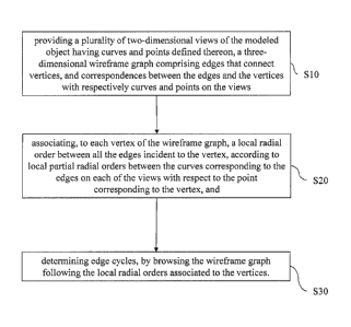
FIG. 1 shows a flowchart of an example of computer-implemented method for
designing a 3D modeled object. The method comprises the step of providing S10
a
plurality of 2D views of the modeled object. The views have curves and points
defined thereon. The method also provides at S10 a 3D wireframe graph. The 3D
wireframe graph comprises edges that connect vertices, and correspondences
between the edges and the vertices with respectively curves and points on the
views.
The method also comprises associating S20, to each vertex of the wireframe
graph, a
local radial order between all the edges incident to the vertex. The
associating S20 is
performed according to local partial radial orders between the curves
corresponding
to the edges on each of the views with respect to the point corresponding to
the
vertex. Then the method comprises determining S30 edge cycles. The determining
S30 is performed by browsing the wireframe graph following the local radial
orders
associated at S20 to the vertices. This improves the design of a 3D modeled
object
based on 2D views of the modeled object.
As explained earlier, the background art considers the provision of a 3D
wireframe graph corresponding to 2D views of a 3D modeled object to be
designed.
However, the user then has to fit the wireframe graph with surfaces manually,
which
is both difficult and may be ambiguous in some cases. The method allows a
robust
automation of the process as it leads to the determination at S30 of edge
cycles on
the 3D wireframe graph. As known in the art, such a 3D wireframe graph with
edge
cycles defined on it may lead to design a surface, by fitting the wireframe
graph with
surfaces based on the determined edge cycles. The method may do that according
to
any known technique, which is not the subject of the present discussion.
CA 02853255 2014-05-30
6
Investigating an algorithm to automate the surfaces creation from the 3D
curves network may thus lead to the problem of finding an appropriate set of
edge
cycles, each edge cycle defining the boundary of a surface as a closed loop of
curves.
Existing algorithms in this field are either combinatorial algorithms or
topological
algorithms. A combinatorial algorithm actually computes a basis of cycles,
typically
a basis of fundamental cycles. In order to avoid surfaces overlapping, a basis
of
minimum cycles is advantageous. Unfortunately, this computation is impractical
for
the following reasons. The algorithmic complexity is polynomial and the basis
of
minimum cycles is not unique, which may lead again to overlapping surfaces, as
illustrated by FIGS. 2-3, which show two different pairs of edge cycles (22
and 24)
or (22 and 26) for the same wireframe graph 20. On the other hand, topological
algorithms require spatial hypotheses on the 3D curve network (mainly the
network
is "almost" planar) that are not realistic in the industrial context.
The method avoids these issues by sorting edges around each vertex in the
appropriate order (the local radial orders involved at the associating S20).
This local
sorting is computed by reusing the input 2D views provided at S10, as each
local
radial order is according to local partial radial orders between the curves on
each of
the views. Traversing the whole 3D curves network according to the local
sorting at
the determining S30 eventually provides a set of edge cycles. Each edge cycle
is a
closed loop of curves and defines the boundary of a surface. Furthermore,
since
cycles' adjacencies are known, tangency constraints may be further handled by
the
method in order to compute tangent resulting surfaces for the fitting
mentioned
above.
The method eliminates the need for manual selection of boundaries for surfaces
creation. This shortens the time to get the virtual 3D object in the CAD
system, and
thus improves productivity. Furthermore, the skin resulting from the method is
guaranteed to be a closed and oriented skin, which in turn improves quality
and,
again, shortens time since a posteriori checking is no longer necessary. When
dealing
with standard input objects, the algorithmic complexity of the method is
linear, and
this is the optimum. Consequently, implementing the method provides the best
possible performance to the CAD system.
A modeled object is any object defined/described by structured data that may
be stored in a data file (i.e. a piece of computer data having a specific
format) and/or
CA 02853255 2014-05-30
=
7
on a memory of a computer system. By extension, the expression "modeled
object"
may designate the data itself The modeled object obtained by the method has a
specific structure, as it has in the data defining it the wireframe graph with
the edge
cycles determined at S30. Moreover, the modeled object may also comprise the
local
radial orders and/or the local partial orders involved at S20, although the
method
may comprise deleting any or both of said local orders once the edge cycles
are
determined at S30.
The method is for designing the 3D modeled object, e.g. the steps of the
method constituting at least some steps of such design. "Designing a 3D
modeled
object" designates any action or series of actions which is at least part of a
process of
elaborating a 3D modeled object. Thus, the method may comprise creating the 3D
modeled object from scratch. Alternatively, the method may comprise providing
a
3D modeled object previously created, and then modifying the 3D modeled
object.
The 3D modeled object may be a CAD modeled object or a part of a CAD
modeled object. In any case, the 3D modeled object designed by the method may
represent the CAD modeled object or at least part of it, e.g. a 3D space
occupied by
the CAD modeled object. A CAD modeled object is any object defined by data
stored in a memory of a CAD system. According to the type of the system, the
modeled objects may be defined by different kinds of data. A CAD system is any
system suitable at least for designing a modeled object on the basis of a
graphical
representation of the modeled object, such as CATIA. Thus, the data defining a
CAD
modeled object comprise data allowing the representation of the modeled object
(e.g.
geometric data, for example including relative positions in space).
The method may be included in a manufacturing process, which may comprise,
after performing the method, producing a physical product corresponding to the
modeled object. In any case, the modeled object designed by the method may
represent a manufacturing object. The modeled object may thus be a modeled
solid
(i.e. a modeled object that represents a solid). The manufacturing object may
be a
product, such as a part, or an assembly of parts. Because the method improves
the
design of the modeled object, the method also improves the manufacturing of a
product and thus increases productivity of the manufacturing process. The
method
can be implemented using a CAM system, such as DELMIA. A CAM system is any
CA 02853255 2014-05-30
8
system suitable at least for defining, simulating and controlling
manufacturing
processes and operations.
The method is computer-implemented. This means that the method is executed
on at least one computer, or any system alike. For example, the method may be
implemented on a CAD system. Thus, steps of the method are performed by the
computer, possibly fully automatically, or, semi-automatically (e.g. steps
which are
triggered by the user and/or steps which involve user-interaction). Notably,
the
providing S10 may be triggered by the user. Other steps of the method may be
performed automatically (i.e. without any user intervention), or semi-
automatically
(i.e. involving, e.g. light, user-intervention, for example for validating
results).
A typical example of computer-implementation of the method is to perform the
method with a system suitable for this purpose. The system may comprise a
memory
having recorded thereon instructions for performing the method. In other
words,
software is already ready on the memory for immediate use. The system is thus
suitable for performing the method without installing any other software. Such
a
system may also comprise at least one processor coupled with the memory for
executing the instructions. In other words, the system comprises instructions
coded
on a memory coupled to the processor, the instructions providing means for
performing the method. Such a system is an efficient tool for designing a 3D
modeled object.
Such a system may be a CAD system. The system may also be a CAE and/or
CAM system, and the CAD modeled object may also be a CAE modeled object
and/or a CAM modeled object. Indeed, CAD, CAE and CAM systems are not
exclusive one of the other, as a modeled object may be defined by data
corresponding to any combination of these systems.
The system may comprise at least one GUI for launching execution of the
instructions, for example by the user. Notably, the GUI may allow the user to
trigger
the step of providing S10, and then, if the user decides to do so, e.g. by
launching a
specific function, to trigger the rest of the method.
The 3D modeled object is 3D (i.e. three-dimensional). This means that the
modeled object is defined by data allowing its 3D representation. Notably, the
wireframe graph is 3D (i.e. the wireframe graph may be non-planar). A 3D
representation allows the viewing of the representation from all angles. For
example,
CA 02853255 2014-05-30
9
the modeled object, when 3D represented, may be handled and turned around any
of
its axes, or around any axis in the screen on which the representation is
displayed.
This notably excludes 2D icons, which are not 3D modeled, even when they
represent something in a 2D perspective. The display of a 3D representation
facilitates design (i.e. increases the speed at which designers statistically
accomplish
their task). This speeds up the manufacturing process in the industry, as the
design of
the products is part of the manufacturing process.
FIG. 4 shows an example of the GUI of a typical CAD system.
The GUI 2100 may be a typical CAD-like interface, having standard menu bars
2110, 2120, as well as bottom and side toolbars 2140, 2150. Such menu and
toolbars
contain a set of user-selectable icons, each icon being associated with one or
more
operations or functions, as known in the art. Some of these icons are
associated with
software tools, adapted for editing and/or working on the 3D modeled object
2000
displayed in the GUI 2100. The software tools may be grouped into workbenches.
Each workbench comprises a subset of software tools. In particular, one of the
workbenches is an edition workbench, suitable for editing geometrical features
of the
modeled product 2000. In operation, a designer may for example pre-select a
part of
the object 2000 and then initiate an operation (e.g. a sculpting operation, or
any other
operation such as a change of dimension, color, etc.) or edit geometrical
constraints
by selecting an appropriate icon. For example, typical CAD operations are the
modeling of the punching or the folding of the 3D modeled object displayed on
the
screen.
The GUI may for example display data 2500 related to the displayed product
2000. In the example of FIG. 4, the data 2500, displayed as a "feature tree",
and their
3D representation 2000 pertain to a brake assembly including brake caliper and
disc.
The GUI may further show various types of graphic tools 2130, 2070, 2080 for
example for facilitating 3D orientation of the object, for triggering a
simulation of an
operation of an edited product or rendering various attributes of the
displayed
product 2000. A cursor 2060 may be controlled by a haptic device to allow the
user
to interact with the graphic tools.
FIG. 5 shows an example of the architecture of the system as a client computer
system, e.g. a workstation of a user.
CA 02853255 2014-05-30
The client computer comprises a central processing unit (CPU) 1010 connected
to an internal communication BUS 1000, a random access memory (RAM) 1070 also
connected to the BUS. The client computer is further provided with a graphics
processing unit (GPU) 1110 which is associated with a video random access
memory
5 1100 connected to the BUS. Video RAM 1100 is also known in the art as
frame
buffer. A mass storage device controller 1020 manages accesses to a mass
memory
device, such as hard drive 1030. Mass memory devices suitable for tangibly
embodying computer program instructions and data include all forms of
nonvolatile
memory, including by way of example semiconductor memory devices, such as
10 EPROM, EEPROM, and flash memory devices; magnetic disks such as internal
hard
disks and removable disks, magneto-optical disks, and CD-ROM disks 1040. Any
of
the foregoing may be supplemented by, or incorporated in, specially designed
ASICs
(application-specific integrated circuits). A network adapter 1050 manages
accesses
to a network 1060. The client computer may also include a haptic device 1090
such
as a cursor control device, a keyboard or the like. A cursor control device is
used in
the client computer to permit the user to selectively position a cursor at any
desired
location on screen 1080, as mentioned with reference to FIG. 4. By screen, it
is
meant any support on which displaying may be performed, such as a computer
monitor. In addition, the cursor control device allows the user to select
various
commands, and input control signals. The cursor control device includes a
number of
signal generation devices for input control signals to system. Typically, a
cursor
control device may be a mouse, the button of the mouse being used to generate
the
signals.
To cause the system to perform the method, it is provided a computer program
comprising instructions for execution by a computer, the instructions
comprising
means for this purpose. The program may for example be implemented in digital
electronic circuitry, or in computer hardware, firmware, software, or in
combinations
of them. Apparatus of the invention may be implemented in a computer program
product tangibly embodied in a machine-readable storage device for execution
by a
programmable processor; and method steps of the invention may be performed by
a
programmable processor executing a program of instructions to perform
functions of
the invention by operating on input data and generating output. The
instructions may
advantageously be implemented in one or more computer programs that are
CA 02853255 2014-05-30
11
executable on a programmable system including at least one programmable
processor coupled to receive data and instructions from, and to transmit data
and
instructions to, a data storage system, at least one input device, and at
least one
output device. The application program may be implemented in a high-level
procedural or object-oriented programming language, or in assembly or machine
language if desired; and in any case, the language may be a compiled or
interpreted
language. The program may be a full installation program, or an update
program. In
the latter case, the program updates an existing CAD system to a state wherein
the
system is suitable for performing the method.
As explained earlier, the method of FIG. 1 is for designing a 3D modeled
object starting from the plurality of 2D views of the modeled object and the
corresponding 3D wireframe graph by determining at S30 the edge cycles. As
explained earlier, the edge cycles may then be used, among other possible
actions
known in the field, for fitting the wireframe graph with surfaces based on
them,
according to any known method. Notably, the surfaces may form a boundary
representation (B-Rep), e.g. under the specific format of B-Reps described in
European patent application No. 12306720.9 which is incorporated herein by
reference. The method may determine at S30 one edge cycle per tile of the
wireframe
graph (referred to as "minimum edge cycle" in the following), such that the
whole set
of edge cycles eventually covers the whole wireframe graph, with no
overlapping.
The views that are provided at S10 are any 2D representations of the 3D
modeled object that is under design. The views may be images. The method may
notably, prior to the providing S10, capture several images of a same single
physical
product that may constitute the views, potentially including some
modifications/additions on the images, as explained below. This may be done
for
example by a camera capturing photos. For example, a same physical product may
be
photographed from different angles, the resulting photos thus representing the
product under different perspectives. In an example, the outer surface of the
physical
product is integrally represented through the plurality of views. The method
may in
such a case reconstruct, or build, a comprehensive 3D design of the physical
product
(or in general any object represented by the views), i.e. the 3D modeled
object, based
on smaller information (2D views) that are however multiple.
CA 02853255 2014-05-30
12
The first step toward this is to consider a 3D wireframe graph that
corresponds
to the plurality of 2D views in a way explained later. The 3D wireframe graph
may
be provided at S10 already prepared as such, or it may be constructed in a
prior step
by the method according to any known technique, e.g. based on the 2D views.
For example, in the case the method comprises capturing images, e.g. photos,
of a same physical product, the method may comprise defining curves and points
on
the images to form the views. In other words, the views are data including a
standard
image with 2D curves and 2D points defined thereon. The curves and points may
be
defined, in any known way, according to the images and the lines and corners
of the
physical product as they appear on the images. The user may be involved in
such a
step, as explained earlier. Known automatic algorithms may also be used. Then,
the
method comprises defining correspondences (in the case of a computer-
implemented
method, correspondences are pieces of data that associate two pieces of data,
such as
links or pointers) between the curves and points of each image with
respectively
curves and points on the other images. Basically, curves and points of
different
images that represent the same lines and corners of the physical product are
put into
correspondence, precisely so as to highlight such information. This may be
performed according to any know method. The user may be involved in such a
step,
as explained earlier. Known automatic algorithms may also be used.
Finally, before the providing S10, the method in such an example constructs
the 3D wireframe graph based on the views and on the correspondences. The 3D
wireframe graph is a graph having a specific structure, according to the
method.
Notably, the wireframe graph comprises as all graphs edges that connect
vertices,
and correspondences between the edges and the vertices with respectively
curves and
points on the views. Furthermore, as known in the field, the edges of the 3D
wireframe graph are associated with 3D curves (also referred to as the edges
in the
following) and the vertices of the 3D wireframe graph are associated to 3D
points or
positions (also referred to as the vertices in the following). In this sense,
with edges
that are 3D curves and vertices that are 3D points defining where the curves
meet on
their ends, the wireframe graph is a three-dimensional modeled object.
The 3D edges and the 3D vertices are determined (when the method comprises
constructing the wireframe graph) based on the views and on the
correspondences
defined earlier. This may be done according to any method known in the art,
and this
CA 02853255 2014-05-30
13
may involve user-interaction and/or known automatic algorithms. Thus, the
wireframe graph is a construction of the modeled object that is based on the
images,
in the sense that different 2D information on the same physical product
contained in
the images is used to reconstruct a 3D wireframe graph corresponding to the
product,
as known per se. For a relatively easy execution of these steps, the physical
product
may be opaque, such that its lines and corners are well defined and such that
there is
no ambiguity among the different 2D views.
The method also comprises associating S20 (i.e. pieces of data representing
such association, e.g. links and/or pointers, are created), to each vertex of
the
wireframe graph, a local radial order between all the edges incident to the
vertex. In
other words, for each vertex of the wireframe graph, all edges incident to the
vertex
are contemplated and an order (local to the vertex) is determined between them
and
stored. The local order is radial, meaning that it represents the order in
which the
edges are encountered when rotating around the vertex. For example, the local
radial
order may radially order the projections of the edges (e.g. a projection of
the tangents
of the edges at the incident vertex) on a plane containing the incident
vertex.
The associating S20 is performed according to local partial radial orders
between the curves corresponding to the edges on each of the views with
respect to
the point corresponding to the vertex. The edges of the wireframe each
correspond to
a respective curve on at least one of the views. Indeed, according to the
perspective
applied by a given view, some edges may not be present on it. However, for
each
edge there is at least one view for which the perspective is such that the
view has a
curve corresponding to the edge defined thereon. Now, considering the set of
edges
incident on each contemplated vertex of the associating S20, all the edges are
present
on at least one of the plurality of views for each of them (via the
corresponding 2D
curves defined on the views). For each such view, a radial order may be
directly
defined between said curves, called "local partial radial order", the view
being 2D.
The associating S20 considers all such local partial radial orders that
correspond to
the set of edges incident on the contemplated vertex and determines the local
radial
order between all edges accordingly, in a systematic way (e.g. the method may
follow a predetermined algorithm to perform the associating), which allows
automation. An example of how to implement this is provided later. Thus, the
method uses at S20 the views to determine such local radial orders for all
vertices of
CA 02853255 2014-05-30
14
the wireframe graph, in addition to a potential previous use of the views to
determine
the wireframe graph. In this sense, the views are efficiently reused for the
automation
of this part of the process.
Then the method comprises determining S30 edge cycles. The determining S30
is performed by browsing the wireframe graph following the local radial orders
associated at S20 to the vertices. In other words, the graph is integrally
traversed (i.e.
edges are followed until all tiles of the wireframe graph are cycled once)
following
the local radial orders. Namely, when browsing the wireframe graph, upon
arriving at
a vertex the local radial order associated at S20 to the vertex is considered
to
determine which edge to follow next (to go to the next vertex). The method may
store the orders in which the edges are thereby followed and define instances
of
cycles (each time the browsing leads to a vertex already visited). This is
illustrated
later. The determining S30 is thus executable in a systematic way and may thus
lead
to a significant automation of the determination of the edge cycles, in a
relatively
simple manner (in terms of computation and memory resources). Said edge cycles
may be used to fit the wireframe graph with surfaces, e.g. a B-Rep, as
explained
earlier.
An example of the method is now discussed with reference to FIGS. 6-XXX,
FIG. 6 showing a flowchart representing the whole method of the discussed
example.
The physical product of the example to model in the CAD system is L-shape
solid 60. The internal edge of the "L" is filleted. The user feeds at S05 the
CAD
system with five 2D pictures (e.g. photos) of this solid (FIGS. 7-11) captured
at S05,
on which curves and points are defined. Camera positions associated with
pictures
are also sent to the CAD system in the example.
The next step of the method of the example is for the user to define and match
up at S06 and S07 points across overlapping pictures (curves being matched up
accordingly). The resulting views are illustrated on FIGS. 12-16 by numerical
labels
which respectively correspond to the five pictures of FIGS. 7-11. Points are
numbered from 1 to 14. Points are tagged with their number on the figures
where
they are visible.
From this information, the CAD system is able to compute at S08 a network of
3D curves (the edges), in other words 3D wireframe graph 170 as illustrated in
FIG.
17. The state of the art technology is able to compute this 3D wireframe
graph. Each
CA 02853255 2014-05-30
vertex and each edge on the 3D wireframe graph corresponds to a point and
curve
that are each visible on at least two input pictures. It is indeed
advantageous to
retrieve the 3D position and shape of an object from more than one 2D
view/picture
of the said object.
5 A goal of the
method of the example is to eventually compute all minimum
edge cycles of this graph at S30, so that the surfaces boundary may
potentially be
defined according to known algorithms. In the context of the example, a
"minimum
edge cycle" is defined as follows. When projected on initial pictures,
oriented edges
of the same minimum cycle correspond to boundary curves of the same 2D face.
10 By
definition, a planar simple loop ("loop" in the following) is a planar closed
curve that separates the plane into exactly two portions. The non-bounded
portion is
named the "outside" of the loop and the bounded portion is named the "inside"
of the
loop.
By definition, a planar face includes one loop named the "external loop" and a
15 set of loops
named "internal loops". The external loop is mandatory while internal
loops are not. Loops are arranged according to the following conditions:
= All internal loops are included inside the external loop.
= No internal loop is included inside another internal loop.
= Considering the set of loops as a planar graph and noting L the number of
loops, E the number of edges, V the number of vertices and K the number
of connected components of the graph, then the following relationship must
be satisfied: L = E ¨V + K .
FIG. 18 illustrates five such minimum edge cycles. FIG. 19 illustrates a cycle
that is not a minimum cycle: some edges are boundary curves of the bottom face
of
the L-shape solid while some others are boundary edges of the back face of the
L-
shape solid.
The method computes all minimum edge cycles through two steps. The first
step is to sort edges around each vertex according to an appropriate
topological local
radial order at S20. The second step is to traverse the 3D graph by using
these radial
orderings at S30.
When the topological radial order is ambiguous, which may happen in
marginal cases, the method of the example provides a strategy ("regularize"
step S28
CA 02853255 2014-05-30
16
on FIG. 6 discussed later) to overcome the difficulty that is reasonably
efficient in
industrial situations.
An example of the associating S20 implemented in the method of FIG. 6 is
now discussed with reference to FIGS. 6-26.
In this example, the associating S20, to each vertex of the wireframe graph,
of
a local radial order between all the edges incident to a respective vertex
comprises
specific actions for each respective vertex that are easily automatable and
lead to
fairly good results. The associating S20 comprises for each respective vertex
determining S22, for each view, the local partial radial order with respect to
the point
corresponding to the respective vertex between curves that are defined on the
view
and that correspond to an edge incident to the respective vertex. In other
words, the
method considers 2D curves on the 2D views that correspond to the edges
incident to
the respective vertex and determines at S22 radial orders thereof on each
view. Then,
the method performs a merging S24 of all the local partial radial orders. All
the local
partial radial orders are thus gathered in one graph. Finally, the method
traverses at
S26 the result of the merging S24 (edges of the merge graph are followed), to
detect
a cycle (one or more) including all the edges incident to the respective
vertex, said
cycle constituting the local radial order associated to the respective vertex.
In the
example, the local partial radial orders are determined at S22 as graphs of
which
nodes identify edges and of which arcs identify subsequence between edges
(i.e. two
edges that are subsequent one to the other on the wireframe graph are linked
by an
oriented arc on the "local partial order" graphs).
Ordering incident edges of a vertex x is performed through two steps. The
first
step is to gather at S22 and S24 around vertex x all partial radial orders
computed
from pictures where it is visible. The second step is to extract at S26 (and
possibly
S28) from all these partial radial orders a unique local radial order.
Given a vertex x, the method of the example finds all views where it is
visible.
For each such view, the method gets the visible edges incident to x, sorts
these
edges around vertex x in a predetermined order (e.g. CCW: counter clockwise)
induced by the planar topology of the picture and stores this partial order in
an
appropriate data structure. For example, vertex 12 of solid 60 is connected to
edges
(12,5), (12,11) and (12,13). The view of FIGS. 8 and 13 features vertex 12
together
with all its connected edges which, additionally, are visible. According to
the planar
CA 02853255 2014-05-30
17
topology of the view of FIGS. 8 and 13, the CCW radial order is then:
((12,5),(12,13),(12,11)) as illustrated in FIG. 20.
Choosing another picture/view featuring same edges connected to vertex x
(picture 4, FIGS 10 and 15, in the example of vertex 12) yields the same
radial order.
This is due to the fact that the 3D object from the real world is bounded by
an
oriented skin. This topological property is captured through the views.
In the L-shape solid example, each vertex is visible together with all its
incident edges from at least one picture, which particularly simplifies the
radial order
computation (because the merging S24 will lead to a uniquely ordered cycle).
This situation does not always occur, and FIGS. 21-26 illustrate a case where
the merging S24 and the traversing S26 help combining the information
determined
at S22.
FIGS. 21-22 illustrate two pictures of a pyramidal V-based solid. Edges
a,b,c,d are incident to the top vertex v of the pyramid. Dotted lines are
invisible
edges, they should not appear on the pictures, but they are represented for
explanation purpose.
In the picture of FIG. 21, vertex v is visible together with incident edges
a,c,d, edge b being hidden. The partial local radial order 230 is then
(a,c,d), as
illustrated in FIG. 23.
In the picture of FIG. 22, vertex v is visible together with incident edges
a,b,c, edge d being hidden. The partial local radial 240 order is then
(a,b,c), as
illustrated in FIG. 24.
Finally, two local partial radial orders are attached to vertex v: order
(a,c,d)
and order (a,b,c) . It must be noticed that there is no starting point in the
order as it
could be understood from parentheses notation. These are cyclic lists in the
example.
For each vertex, the local radial order is obtained at S20 by combining and
analyzing at S26 local partial radial orders. Back to the V-based solid
example,
vertex v is associated with local partial radial orders (a,c,d) and (a,b,c).
The first
step is to merge at S26 all local partial radial orders into a single graph
250, as
illustrated on FIG. 25. It must be understood that the vertices a,b,c,d of
partial radial
order graphs are edges of the 3D wireframe graph and that oriented arcs of
partial
radial order graphs capture partial radial orders around vertex v.
CA 02853255 2014-05-30
18
Then, the resulting oriented graph is analyzed to check if it includes a
maximum and unique cycle ("maximum" meaning that the cycle includes all
nodes).
The algorithm is to build the graph traversal starting from an arbitrary node.
FIG. 26
illustrates the graph traversal starting from node a, which yields a tree 260
rooted at
node a. Classically, graph traversal is interrupted when a node of the current
branch
is previously visited (a branch being a path of arcs starting at the root
node). The
resulting rooted tree 260 is illustrated in FIG. 26.
Tree 260 collects all cycles of the graph as follows: each path from the root
node to a leaf node is a cycle. It is clear in this example that there exists
only one
maximum cycle which is (a,b,c,d) and illustrated with boxed letters. This
cycle is
the local radial order of edges around vertex v retained by the method of the
example. It may happen that the maximum cycle is not unique, thus leading to
ambiguity. This situation is detailed later.
An example of the determining S30 implemented in the method of FIG. 6 is
now discussed.
In this example, determining (S30) edge cycles by browsing the wireframe
graph comprises the sub-steps of chosing a vertex and forming an edge list
starting
from the chosen vertex, and repeating said sub-steps. In other words, vertices
are
repeatedly chosen and edge lists are formed each time a vertex is chosen, e.g.
until
all minimal edge lists are determined.
Forming the edge list is performed by following, starting from the chosen
vertex, the local radial orders associated to the vertices as they are
encountered. In
other words, when the algorithm is at a vertex, the algorithm retrieves the
first edge
provided by the local radial order associated to said vertex (e.g. the method
marks
edges of the local radial orders as used, such that the algorithm retrieves
the first
unused edge of the local radial order). Then, the algorithm goes to the other
vertex
connected to said edge. The algorithm increments the edge list with such
followed
edges, until the edge list forms an edge cycle. This allows a fast and
efficient
determination at S30.
A detailed implementation is provided with reference to FIG. 27.
As can be seen, in the implementation of FIG. 27, determining S30 edge cycles
by browsing the wireframe graph comprises the sub-steps of:
= chosing a vertex x vertices marked as unused,
CA 02853255 2014-05-30
19
= initializing an edge list L, by selecting an edge e starting at vertex x,
= adding output edge e of said vertex x to the edge list L and marking the
added
output edge e as used,
= if the added output edge e of said vertex is the last unused output edge
of
said vertex x, marking said vertex x as used,
= incrementing the edge list L by following the edges according to the
local
radial orders associated to the vertices as they are encountered, until the
edge
list L forms an edge cycle, and
= repeating the preceding sub-steps, discarding vertices and edges marked
as
used.
The input data for 3D wireframe graph traversal are the 3D wireframe graph
together with local radial orders at each vertex. The output data is the list
of all
minimum cycles of the 3D graph. The following preprocessing is advantageous:
all
edges of the 3D graph are duplicated and oriented in opposite directions. By
definition, an oriented edge is "used" if it is involved in a minimum cycle. A
vertex
is "used" if all its output edges are used in minimum cycles. Before the
algorithm
starts, all edges and all vertices are "unused". At the end of the algorithm,
each
oriented edge is involved in one and only one minimum cycle. The graph
traversal
algorithm is described in the diagram of FIG. 27.
Instruction " e := Next ( e , y ) " uses the local radial order of edges
around
vertices. Function "b = Next ( a, v )" yields the edge "b" starting at vertex
"v" and
preceding edge "a" according to the local radial order of edges around vertex
"v".
As can be seen, the method takes advantage of the local radial orders so that,
with a simple but smart marking of vertices and edges as used or unused (after
the
duplication), the method may easily and efficiently perform the determination
S30 of
all minimal edge cycles.
The special case of a non-unique local radial order is now discussed with
reference to FIGS. 28-40.
This is the case when the traversing S26 of the result of the merging S24 of
all
the local partial radial orders leads to detecting several (different) cycles
including all
the edges incident to the respective vertex.
A non-unique local radial order may occur as explained in the following. The
example solid is a tetrahedron, as illustrated on FIG. 28. Four pictures of
the
CA 02853255 2014-05-30
tetrahedron are given in such a way that only one face is visible on each
picture.
Each visible face hides all three other faces of the tetrahedron, as
illustrated by FIG.
29.
Given a vertex v, only two incident edges are visible on each picture. Noting
5 a,b,c the three incident edges at vertex v, local partial orders are
meaningless since
they organize a cyclic list of two objects, as illustrated on FIGS. 30-32
which show
local partial orders 300, 310 and 320.
Merging all local partial orders yields a directed graph from which the cycle
analysis finds two cycles in opposite orders (a,b,c) and (a,c,b), as on FIG.
33.
10 Clearly, this is not finished.
The method of the example may solve this issue by selecting S28 one of the
cycles detected for such a vertex having several different local radial orders
(potentially) associated to it, and referred to as "singular" vertex. The
method thus
selects one cycle as the local radial order used in the determining S30. The
method
15 may further comprise marking the vertex as a singular vertex (after the
traversal
S26), for later use of such information.
Notably, the selecting S28 may be performed indirectly. The selecting S28 one
of the cycles detected may indeed comprise performing a regularization process
(which is iterative) on the set of all singular vertices.
20 The regularization process comprises chosing a starting singular vertex
and a
starting output edge (an edge incident to the chosen singular vertex) of said
starting
singular vertex. This chosing may be performed in any way. Then the
regularization
process comprises browsing the wireframe graph following the local radial
orders
associated to the vertices (i.e. the first edge of the local radial order
associated to an
edge is followed each time the algorithm arrives at a vertex), in order to
detect an
edge cycle at said starting singular vertex. Then if the browsing
reaches/leads to
another singular vertex, the method repeats the regularization process with a
new
starting singular vertex and/or a new starting output edge (the browsing is
indeed
facing an ambiguity and the proposed way to solve this ambiguity is to restart
somewhere else). Else (i.e. if an edge cycle is detected with no other
singular vertex
encountered), the method may associate to said starting singular vertex the
cycle, that
was detected at S26, and that is compliant with the order between the starting
output
edge and the final edge browsed (the other potential local radial order(s)
that are
CA 02853255 2014-05-30
21
provided by the other cycles detected at S26 in competition are discarded). In
other
words, the local radial order that is retained is the one in which the
starting edge and
the ending edge of the cycle detected during the regularization (both edges
being
incident to the singular vertex under regularization) are ordered correctly
(i.e. in the
same order as for the detected cycle). Then the method removes the starting
singular
vertex from the set of all singular vertices (indeed, the singular vertex has
been
regularized as a unique local radial order has been retained for it), and then
repeats
the regularization process. This algorithm is executed until no singular
vertex
remains. Examples are discussed hereunder.
Despite vertices featuring a non-unique local radial order are marginal in
images of real life objects, they would better not be ignored. In fact, it is
possible to
deal with them, generally provided they are not too numerous. (Obviously, in
the rare
case the method does not manage to regularize the wireframe graph, then it can
simply be discarded.) A vertex featuring a non-unique radial order is called a
singular vertex in the following.
The principle is as follows. Suppose that all possible local radial orders are
computed and start a cycle computation at a singular vertex x. Since the
starting
edge of the cycle, noted u, is arbitrarily chosen among output edges of x,
singularity is not a trouble. If no other singular vertex is encountered while
computing the cycle, the algorithm ends the said cycle with an edge v that is
an
input edge of vertex x. So, it is clear that the appropriate radial order
around vertex
x is the one featuring the sequence u, v as opposed to the one featuring the
sequence
v, u. Consequently, it is possible to regularize vertex x by setting the
correct local
radial order. Then, the strategy is to identify singular vertices while
computing local
radial orders and to regularize them as much as possible.
The regularization algorithm is as shown on FIG. 34. After local radial orders
are computed, all singular vertices are stored in an initial list L. The main
loop is to
iteratively remove singular vertices from list L. Iterations are stopped when
no
singular vertex can be removed.
If the resulting list is not empty, it includes unavoidable singular vertices
and
cycle computation is not possible. Otherwise, all singular vertices are
removed and
all local radial orders are unique. The cycles computation described
previously will
be successful.
CA 02853255 2014-05-30
22
Function Reg(L) tries to regularize each singular vertex of the input list L.
It
modifies list L by removing elements and decreasing its size. If at least one
vertex is
regularized, there is a chance that a new try regularizes some others, which
validates
iterations. Function Reg(L) is as follows:
Function Reg(L)
For each vertex x L do begin
If vertex x is regularized then
Remove x from list L
End if
End for
Return L
Regularizing vertex x in function Reg(L) is to search a cycle starting at
vertex
x including only regular vertices but x . This is performed as described in
the
diagram of FIG. 35.
Regularization is exemplified by solid 360 of FIG. 36.
FIGS. 37-39 illustrate three input images of solid 360 of FIG. 36. Notice that
hidden lines are represented as dotted lines for clarity and should not appear
on
images. Vertex 4 is not visible on the image of FIG. 37. Vertex 3 is not
visible on the
image of FIG. 38. Vertex 2 is not visible on the image of FIG. 39.
Computed local radial orders are illustrated on FIG. 40. Vertices 1 and 5 are
singular since radial orders could not be oriented. It should be noticed that
initializing a cycle computation at a regular vertex always fails because any
cycle
include either vertex 1 or vertex 5, which are singular so far.
The list of singular vertices includes 1 and 5. Regularization starts with
vertex
1. Choosing edge (1,3) leads to vertex 3, which is regular. Thanks to local
ordering at
vertex 3, next edge is (3,4) leading to vertex 4, which is regular. Thanks to
local
ordering at vertex 4, next edge is (4,1) closing the cycle at vertex 1.
Clearly, the
appropriate local ordering at vertex 1 is (1,3),(1,4),(1,2) changing it into a
regular
vertex. Singular vertex 5 is regularized the same way. Then, computation of
all
cycles is possible.
The algorithmic complexity of the method is now discussed.
CA 02853255 2014-05-30
23
Let V ,E respectively the number of vertices and edges of the 3D wireframe
graph and F the number of faces of the input object, which is also the number
of
minimum cycles. Let E. the largest number of edges incident to a vertex.
Despite
E. can be made proportional to E with particular solids, real life objects
feature a
small and constant E.. The previously discussed L-shape solid 60 is such that
E. =3 , the previous V-based pyramid is such that E. = 4. The algorithmic
complexity of the local ordering is bounded by V x Sorting(E.) where function
Sorting() is the complexity of the sorting algorithm, typically Sorting(n)= n
log n,
or Sorting(n)= n2. The algorithmic complexity of graph traversal is
proportional to
E since each edge is visited twice. Finally, when dealing with regular input
objects,
the overall complexity of the algorithm is linear, meaning that it is
proportional to
aE + bV where a,b are constant numbers.
Singularity management marginally affects linearity since the regularization
complexity if bounded by S x V. x F where S is the number of singular
vertices.
Thanks to Euler relations of connected topological graphs V ¨ E + F = 2(1¨ G)
(number G is the genus), the number of faces (that is the number of minimum
cycles) is a linear combination of the number of vertices and edges. This
proves that
the algorithm of the method is optimal from the algorithmic complexity point
of
view.