Note: Descriptions are shown in the official language in which they were submitted.
CA 02864807 2014-08-15
WO 2013/123293
PCT/US2013/026289
INVERSION-BASED CALIBRATION
OF DOWNHOLE ELECTROMAGNETIC TOOLS
FIELD OF THE INVENTION
[0001] Disclosed embodiments relate generally to calibration methods for
downhole
electromagnetic measurement tools and more particularly to inversion-based
methods for
calibrating downhole electromagnetic measurement tools.
BACKGROUND INFORMATION
[0002] The use of electromagnetic measurements in prior art downhole
applications,
such as logging while drilling (LWD) and wireline logging applications is well
known.
Such techniques may be utilized to determine a subterranean formation
resistivity, which,
along with formation porosity measurements, is often used to indicate the
presence of
hydrocarbons in the formation. Moreover, azimuthally sensitive directional
resistivity
measurements are commonly employed, e.g., in pay-zone steering applications,
to
provide information upon which steering decisions may be made. Directional
resistivity
tools often make use of tilted or transverse antennas (antennas that have a
magnetic dipole
that is tilted or transverse with respect to the tool axis).
[0003] Tool calibration is an important and necessary task in electromagnetic
logging
operations. Factors such as imperfections in tool construction and variations
due to tool
electronics can introduce significant measurement errors. The intent of tool
calibration is
to eliminate and/or compensate for the effects of these factors on the
measurement data.
Various tool compensation methods are known. For example, air calibration
methods are
1
CA 02864807 2014-08-15
WO 2013/123293
PCT/US2013/026289
commonly employed. In such methods, an electromagnetic resistivity tool may be
suspended (e.g. via crane) in air away from any conducting media. A
resistivity
measurement should yield near-infinite resistivity (i.e., a conductivity of
zero). Any
deviation is subtracted and is assumed to be related to systematic measurement
errors
(e.g., related to the electronics, hardware, or processing methods). U.S.
Patents 4,800,496
and 7,027,923 disclose methods for determining a sonde error in induction or
propagation
logging tools that require measurements to be made at two or more heights
above the
surface of the earth.
[0004] While the aforementioned calibration methods may provide an adequate
calibration for conventional electromagnetic logging tools, they can be
difficult to
implement with deep reading, directional electromagnetic resistivity tools
(look-around
tools) or electromagnetic look-ahead tools. As described in more detail below,
the
transmitter and receiver subs in such deep reading tools are modular such that
neither the
axial spacing nor the azimuthal alignment angle between the subs are fixed.
Hence a
calibration performed for one tool configuration will not necessarily be valid
for any
other tool configuration. Moreover, performing a conventional air calibration
tends to be
difficult if not impossible to implement at a drilling site owing to the long
spacing
between transmitter and receiver subs (e.g., up to 100 feet or more) and the
need to
suspend the entire BHA. Therefore, there remains a need in the art for an
improved
system for calibrating directional resistivity logging tools.
2
CA 02864807 2014-08-15
WO 2013/123293
PCT/US2013/026289
SUMMARY
[0005] An inversion-based calibration method for downhole electromagnetic
tools is
disclosed. Electromagnetic data are acquired in a subterranean borehole using
a least one
measurement array (e.g., at least one transmitter receiver pair). An inversion
of a
formation model (also referred to in the art as a forward model) is processed
to obtain
formation parameters and at least one calibration parameter for the
measurement array.
The calibration parameter for the measurement array may then be fixed and the
inversion
processed again to obtain formation parameters and at least one calibration
parameter for
a second measurement array. This procedure may be repeated recursively for
substantially any number of measurement arrays.
[0006] The disclosed embodiments may provide various technical advantages. For
example, the disclosed embodiments provide a viable calibration methodology
for
modular deep reading and/or look ahead electromagnetic measurement tools. The
disclosed methods may further advantageously be applied to substantially any
electromagnetic measurement system. Moreover, the measurement tools may be
advantageously recalibrated at substantially any time during an
electromagnetic logging
operation without removing the tool from the subterranean environment. Such re-
calibration may be useful, for example, if the average level of resistivity
changes, e.g.,
when the tool enters the highly-resistive area in which the higher-frequency
measurements become more sensitive.
[0007] This summary is provided to introduce a selection of concepts that are
further
described below in the detailed description. This summary is not intended to
identify key
3
CA 02864807 2014-08-15
WO 2013/123293
PCT/US2013/026289
or essential features of the claimed subject matter, nor is it intended to be
used as an aid
in limiting the scope of the claimed subject matter.
BRIEF DESCRIPTION OF THE DRAWINGS
[0008] For a more complete understanding of the disclosed subject matter, and
advantages thereof, reference is now made to the following descriptions taken
in
conjunction with the accompanying drawings, in which:
[0009] FIG. 1 depicts one example of a rig on which disclosed tool and method
embodiments may be utilized.
[0010] FIG. 2A further depicts the deep reading resistivity tool configuration
shown on
FIG. 1.
[0011] FIG. 2B depicts a look ahead resistivity tool configuration.
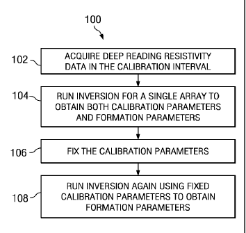
[0012] FIG. 3 depicts a flow chart of one disclosed method embodiment.
[0013] FIG. 4 depicts a flow chart of another disclosed method embodiment.
[0014] FIGS. 5A, 5B, and 5C depict resistivity maps for an experimental test
in which a
deep reading look-ahead resistivity tool is suspended vertically above the
surface of the
earth. A first control is depicted on FIG. 5A in which no calibration shifts
were used in
the inversion, a second control on FIG. 5B in which upper point values were
used to
compute approximate air calibration shifts, and a comparison on FIG. 5C in
which the
calibration shifts were computed using the calibration inversion methods
depicted on
FIGS. 3 and 4.
[0015] FIG. 6 depicts a resistivity log for an example formation.
4
CA 02864807 2014-08-15
WO 2013/123293
PCT/US2013/026289
[0016] FIGS. 7A, 7B, 7C, and 7D depict resistivity maps for an experimental
test in
which a deep reading look-ahead resistivity tool is deployed in subterranean
borehole.
The maps depicted on FIGS. 7A and 7C were generated using synthetic data
needing no
calibration. The maps depicted on FIGS. 7B and 7D were generated using the
inversion
calibration methods described herein with respect to FIGS. 3 and 4 and a first
portion of
the log data shown on FIG. 6.
[0017] FIGS. 8A, 8B, 8C, and 8D depict resistivity maps for an experimental
test in
which a deep reading look-ahead resistivity tool is deployed in subterranean
borehole.
The maps depicted on FIGS. 8A and 8C were generated using synthetic data
needing no
calibration. The maps depicted on FIGS. 8B and 8D were generated using the
inversion
calibration methods described herein with respect to FIGS. 3 and 4 and a
second portion
of the log data shown on FIG. 6.
DETAILED DESCRIPTION
[0018] FIG. 1 depicts an example drilling rig 10 suitable for employing
various method
embodiments disclosed herein. A semisubmersible drilling platform 12 is
positioned over
an oil or gas formation (not shown) disposed below the sea floor 16. A subsea
conduit 18
extends from deck 20 of platform 12 to a wellhead installation 22. The
platform may
include a derrick and a hoisting apparatus for raising and lowering a drill
string 30,
which, as shown, extends into borehole 40 and includes a drill bit 32 deployed
at the
lower end of a bottom hole assembly (BHA) that further includes a modular
electromagnetic measurement tool 50 suitable for making deep reading
resistivity
CA 02864807 2014-08-15
WO 2013/123293
PCT/US2013/026289
measurements. In the depicted embodiment, the modular electromagnetic
measurement
tool 50 includes a conventional electromagnetic logging tool 60 (e.g., an
induction/propagation logging tool) and several electromagnetic measurement
modules
(subs) 52, 54, and 56 deployed in the BHA. Example tool configurations are
described in
more detail below with respect to FIGS. 2A and 2B.
[0019] It will be understood that the deployment illustrated on FIG. 1 is
merely an
example. Drill string 30 may include substantially any suitable downhole tool
components, for example, including a steering tool such as a rotary steerable
tool, a
downhole telemetry system, and one or more measure-while-drilling (MWD) or
logging-
while-drilling (LWD) tools including various sensors for sensing downhole
characteristics of the borehole and the surrounding formation. Moreover, as
described in
more detail below, measurement modules 52, 54, and 56 may be interspersed
between
various ones of such downhole tools (e.g., between a steering tool and an MWD
tool).
The disclosed embodiments are by no means limited in these regards.
[0020] It will be further understood that disclosed embodiments are not
limited to use
with a semisubmersible platform 12 as illustrated on FIG. 1. The disclosed
embodiments
are equally well suited for use with either onshore or offshore subterranean
operations.
Moreover, it will be appreciated that the terms borehole and wellbore are used
interchangeably herein.
[0021] FIG. 2 depicts one example of a deep reading electromagnetic
measurement tool
50. As described in U.S. Patent Publication 2011/0133740 (which is fully
incorporated
by reference herein), modular tool configurations may be used to obtain deep
reading
6
CA 02864807 2014-08-15
WO 2013/123293
PCT/US2013/026289
resistivity data. Such modular designs allow the transmitter and receiver
antennas to be
placed at various locations within a BHA, or at locations in the drill string
above the
BHA. For example, in the tool configuration shown on FIG. 2 the BHA may
include four
receiver modules 52, 54, 56, and 58 and one transmitter module 51 deployed in
the drill
string among other downhole tools 60, 62, 64, and 66. In the depicted
embodiment
downhole tool 60 includes an electromagnetic logging while drilling tool used
to evaluate
formation resistivity, resistivity anisotropy, and dip. Tools 62, 64, and 66
may include
other LWD tools, MWD tools, and the like. By inserting transmitter and/or
receiver
modules at different locations on a standard BHA, as shown in FIG. 2, or a
drill string,
specific depths of investigation can be implemented to improve the formation
model
inversion process used to process such deep resistivity measurements. For
example, in
one embodiment, transmitter module 56 may be about 100 feet from transmitter
module
51.
[0022] It will be understood that modules 51, 52, 54, 56, and 58 may include
one or
more transmitting antennas, receiving antennas, or transceiver antennas. In
such
transceiver embodiments, the antennas are not designed as separate
transmitters or
receivers. Instead, the same antenna may function as either a transmitter or a
receiver.
Such enhancement, besides being economically advantageous, allows more depth
of
investigation for the same number of transceiver modules.
[0023] Directional electromagnetic logging tools commonly use axial,
transverse,
and/or tilted antennas. An axial antenna is one whose dipole moment is
substantially
parallel with the longitudinal axis of the tool. Axial antennas are commonly
wound about
7
CA 02864807 2014-08-15
WO 2013/123293
PCT/US2013/026289
the circumference of the logging tool such that the plane of the antenna is
orthogonal to
the tool axis. Axial antennas produce a radiation pattern that is equivalent
to a dipole
along the axis of the tool (by convention the z direction). A transverse
antenna is one
whose dipole moment is substantially perpendicular to the longitudinal axis of
the tool. A
transverse antenna may include a saddle coil (e.g., as disclosed in U.S.
Patent
Publications 2011/0074427 and 2011/0238312) and generate a radiation pattern
that is
equivalent to a dipole that is perpendicular to the axis of the tool (by
convention the x or y
direction). A tilted antenna is one whose dipole moment is neither parallel
nor
perpendicular to the longitudinal axis of the tool. Tilted antennas are well
known in the
art and commonly generate a mixed mode radiation pattern (i.e., a radiation
pattern in
which the dipole moment is neither parallel nor perpendicular with the tool
axis).
[0024] Triaxial antenna sensor arrangements are also commonly utilized. A
triaxial
antenna arrangement (also referred to as a triaxial transmitter, receiver, or
transceiver) is
one in which two or three antennas (i.e., up to three distinct antenna coils)
are arranged to
be mutually independent. By mutually independent it is meant that the dipole
moment of
any one of the antennas does not lie in the plane formed by the dipole moments
of the
other antennas. Three tilted antennae is one common example of a triaxial
antenna
sensor. Three collocated orthogonal antennas, with one antenna axial and the
other two
transverse, is another common example of a triaxial antenna sensor. While
certain
antenna configurations have been described herein, it will be understood that
the
disclosed embodiments are not limited to any particular antenna configuration.
8
CA 02864807 2014-08-15
WO 2013/123293
PCT/US2013/026289
[0025] FIG. 2B an alternative electromagnetic measurement tool embodiment for
making look-ahead directional resistivity measurements. The depicted
embodiment is
similar to that shown on FIG. 2A in that it includes electromagnetic
measurement
modules 51, 52, 54, and 56. While disclosed embodiments are in no way limited
in this
regard, the depicted embodiment may include BHA may include first, second, and
third
receiver modules 52, 54, and 56 and transmitter module 51 deployed in the BHA.
Those
of skill in the art will readily appreciate that locating the transmitter near
the drill bit tends
to facilitate the look-ahead electromagnetic measurements.
[0026] Owing to the modular nature of the deep reading resistivity tools
described
above with respect to FIGS. 2A and 2B, neither the axial spacing nor the
azimuthal
alignment angle between the various antenna modules are fixed from one logging
operation to the next. Thus any tool calibration is typically only valid for a
particular
tool/BHA configuration. In other words a calibration for any particular tool
configuration
(e.g., the configurations shown on FIGS. 2A and 2B) is only valid for that
particular tool
configuration and is generally not valid for any other configuration. As a
result, modular
deep reading resistivity tools generally need calibration prior to every
logging operation
(i.e., after the BHA is made up with the various antenna modules thereby
fixing the
antenna spacings for that operation). Such
calibration requirements tend to be
excessively burdensome using prior art calibration techniques.
[0027] FIG. 3 depicts a flow chart of one disclosed method embodiment 100. A
drill
string including an electromagnetic measurement tool (e.g., including a
modular deep
reading resistivity tool or a look ahead resistivity tool as depicted on FIGS.
2A and 2B) is
9
CA 02864807 2014-08-15
WO 2013/123293
PCT/US2013/026289
deployed in a subterranean wellbore. Resistivity data (such as deep reading or
look ahead
resistivity data) are acquired at 102 in at least a calibration interval of
the wellbore (e.g.,
in a preselected region of the wellbore). The calibration interval may be
preselected
based on any number of factors, for example, including operator convenience
and/or
previously characterized electrical properties of the formation. It may be
advantageous to
a select a calibration interval having a near constant resistivity (i.e.,
being substantially
free of contrast boundaries) so as to simplify the formation model and reduce
the number
of inversion parameters used in the model. In addition, to reduce uncertainty
due to tool
bending and change in inclination of transmitter and receiver subs, it may
further be
advantageous to perform calibration on a straight trajectory interval. A
region of high
resistivity may also be advantageous so as to minimize the formation response
as
compared to the calibration parameters in the subsequent inversion. Moreover,
for
drilling operator convenience it may be desirable to select a calibration
interval at the
beginning of a well placement or logging job prior to approaching the region
of interest
from which the resistivity data are to be acquired.
[0028] As described in more detail below, the acquired data includes sensor
data from
at least a first measurement array (i.e., a transmitter having at least one
transmitting
antenna spaced apart from a receiver having at least one receiving antenna).
The acquired
data may include substantially any coupling in the voltage tensor. For
example, when
using directional transmitter and receiver arrangements, the acquired data may
include
selected couplings from the following voltage tensor:
CA 02864807 2014-08-15
WO 2013/123293
PCT/US2013/026289
V Vxz\
= V V V
yx yy yz
V V V
\µ. zx zy zz
[0029] wherein the first index (x, y, or z) refers to the transmitter dipole
and the second
index refers to the receiver dipole. By convention, the x and y indices refer
to transverse
moments while the z index refers to an axial moment. The disclosed embodiments
are of
course not limited to any particular conventions. Nor are they limited to
using purely
axial or purely transverse transmitter and/or receiver antennas.
[0030] The acquired data may also include various measurements that are
derived from
the antenna couplings. These measurements may include, for example,
symmetrized
directional amplitude and phase (USDA and USDP), anti-symmetrized directional
amplitude and phase (UADA and UADP), harmonic resistivity amplitude and phase
(UHRA and UHRP) and harmonic anisotropy amplitude and phase (UHAA and UHAP).
These parameters are known to those of ordinary skill in the art and may be
derived from
the antenna couplings, for example, as follows:
USDA= 20logio zz zx zz xz
Vzz + Vz, Vzz ¨ V,z
V ¨ +V
USDP = ¨angle zz V zx V= xz
Vzz + Vz, Vzz ¨ V,z
V ¨ V V ¨V
UADA= 20logio zz . xz
Vzz + Vz, Vzz + V,z
V V V ¨V
¨
UADP = ¨angle zz = xz
Vzz + Vz, Vzz + V,z
11
CA 02864807 2014-08-15
WO 2013/123293
PCT/US2013/026289
¨ 2Vzz
UHRA= 20logio _____________________________
/ + V
xx YY
(
¨ zz
UHRP = ¨angle 2V
/ + V
xx YY
(
V
UHAA= 20logio
V
)Y
(V
UHAP = ¨angle
V)
[0031] Note that the above list is by no means exhaustive and that other
derived
parameters may be acquired at 102. Note also that with the exception of UHRA
and
UHRP, the measurements include cross coupling components (e.g., Võz and Vzõ).
Since
there is minimal cross coupling in homogeneous media, USDA, USDP, UHAA, UHAP,
UADA, and UADP reduce to zero (or near zero) in the absence of boundary layers
or
other heterogeneities.
[0032] With continued reference to FIG. 3, a mathematical inversion is
processed for
data collected from a single measurement array at 104 and is used to obtain
calibration
parameters for the measurement array and various formation parameters (the
particular
formation parameters depending on the configuration of the formation model).
The
obtained calibration parameters may be fixed in the formation model at 106 and
the
inversion is processed again at 108 using the fixed calibration parameters for
the first
measurement array to obtain the various formation parameters. At 108 the
inversion may
12
CA 02864807 2014-08-15
WO 2013/123293
PCT/US2013/026289
be processed for logging data acquired over the entire logging interval to
obtain the
formation parameters (as the calibration parameters have been fixed at 106).
[0033] FIG. 4 depicts a flow chart of another disclosed method embodiment 150.
As
with method 100, deep reading resistivity data are acquired in the calibration
interval at
102. The deep reading resistivity data may be collected at substantially any
suitable
number of measurement arrays (e.g., using multiple pairs of
transmitter/receiver modules
in the tool embodiment depicted on FIG. 2 ¨ each transmitter/receiver module
including
at least one antenna). Moreover, shallow reading resistivity data may also be
acquired
(e.g., using electromagnetic logging tool 60 shown on FIG. 2). An inversion is
processed
at 154 for the data acquired by the first measurement array to obtain
calibration
parameters for both the first measurement array and various formation
parameters. The
obtained calibration parameters may be fixed at 156 and the inversion
processed again at
158 for the data acquired by the first and second measurement arrays (e.g., by
the first
and second pairs of modules having corresponding first and second axial
spacings along
the BHA) to obtain calibration parameters for the second measurement array and
the
various formation parameters. In the illustrated embodiment, the first
measurement array
may have a shorter axial spacing relative to the axial spacing of second
measurement
array (e.g., the first measurement array may have a "short spacing" and the
second
measurement array may have a "long spacing"). The obtained calibration
parameters for
the second measurement array may then fixed at 160 and the inversion may
processed
again at 162 using the fixed calibration parameters for the first and second
measurement
arrays to obtain the various formation parameters. At 162 the inversion may be
processed
13
CA 02864807 2014-08-15
WO 2013/123293
PCT/US2013/026289
for logging data acquired over the entire logging interval to obtain the
formation
parameters (as the calibration parameters have been fixed at 160).
[0034] In embodiments in which a tool configuration including three or more
measurement arrays is utilized, the above process may be repeated recursively.
For
example, when a third measurement array is used, the inversion may be
processed again
for the data acquired at the first, second, and third measurement arrays to
obtain
calibration parameters for the third measurement array and the various
formation
parameters. The obtained calibration parameters for the third measurement
array may
then be fixed. Fourth, fifth, and any subsequent measurement arrays
(correspondingly
spaced along the axis of the BHA) may be calibrated recursively in the same
manner. In
such operations involving multiple calibrations, it may be advantageous to
begin with the
short spacing measurement arrays and work upwards to the longer spacing
arrays.
[0035] Those of ordinary skill in the art will readily appreciate that
inversion is a
mathematical process by which data (in this particular case electromagnetic
logging data)
are used to generate a formation model or to obtain model parameters that are
consistent
with the data. In a conventional inversion process a formation model is
provided that
includes various formation parameters such as the resistivity profile of the
formation
crossed by the tool, distances to one or more boundary layers, resistivity of
one or more
remote beds, vertical and horizontal resistivity of various beds, an
anisotropy ratio,
boundary layer dip angle, and the like. A relatively simple formation model
may include,
for example, a near bed resistivity, a remote bed resistivity, and a distance
to the
boundary between the near and far beds. More complex formation models may
include
14
CA 02864807 2014-08-15
WO 2013/123293
PCT/US2013/026289
three or more beds, vertical and horizontal resistivity values for each of the
beds, and dip
angles between the formation boundaries and the axis of the logging tool.
Moreover, the
beds may be ahead of the bit (e.g., in a look ahead logging operation) or
adjacent to the
logging tool (in a look around logging operation). Processing the inversion is
the
computerized process by which the calibration parameter values (or shifts) and
the
formation parameter values are obtained so as to mathematically fit the
measured data
(e.g., the voltage tensor or the USDA, USDP, UHAA, UHAP, UHRA, UHRP, UHRA,
and UHRP values described above) with minimal error (or error within
preselected
tolerances).
[0036] In disclosed method embodiments 100 and 150, the formation model is
configured so as to further include calibration parameters for selected
measurement
arrays. The calibration parameters may include, for example, calibration
parameters (or
shifts) for UHRA and UHRP. The calibration parameters may
alternatively/additionally
include real and imaginary components of the harmonic resistivity (or other
resistivity
parameters). Moreover, the calibration parameters may include calibration
parameters (or
shifts) for certain ones of the aforementioned voltage measurements (e.g., VL,
,
and/or c). The disclosed embodiments are not limited in this regard. In
embodiments
in which electromagnetic measurements are made at multiple frequencies, the
calibration
parameters may include one or more parameters (e.g., a UHRA and a UHRP shift)
for
each frequency. Thus in one non-limiting example in which six frequencies are
utilized
for a given transmitter receiver pair, there may be a total of twelve unknown
calibration
CA 02864807 2014-08-15
WO 2013/123293
PCT/US2013/026289
parameters in the inversion (six UHRA and six UHRP shifts). Again, the
disclosed
embodiments are not limited to any particular number of frequencies.
[0037] It will be understood that the disclosed embodiments are not limited to
any
particular formation model. Nor are the disclosed embodiments limited to any
particular
mathematical techniques for processing the inversion. Rather, substantially
any suitable
algorithmic means may be used to obtain values for the calibration parameters
and the
formation parameters and to minimize the error between the measured tool
responses and
the formation modelled responses. Those of ordinary skill will readily be able
to
implement various mathematical inversion techniques, for example, including
deterministic Gauss-Newton inversion and stochastic Monte-Carlo inversion
methods.
[0038] While the disclosed embodiments are not limited to any particular
formation
model, it may be advantageous to select a calibration interval in which the
formation has
substantially homogeneous electrical properties (in which there are no
boundaries). The
absence of boundaries and other heterogeneities tends to significantly reduce
the number
of formation parameters in the formation model and therefore tends to simplify
and
improve the calibration parameters determined by the inversion. Moreover, it
may be
further advantageous to select a high resistivity region such that the tool
response is
similar to that of an air calibration. However, the disclosed embodiments are
not limited
in these regards.
[0039] The disclosed embodiments are now described in further detail with
respect to
the following non-limiting examples. FIGS. 5A, 5B, and 5C depict resistivity
maps for
an experimental test in which a deep reading look-ahead resistivity tool is
suspended
16
CA 02864807 2014-08-15
WO 2013/123293
PCT/US2013/026289
(e.g., using a crane) vertically above the surface of the earth. Such
resistivity maps are
described in more detail in U.S. Patent Application Serial Number 13/312,205.
A number
of measurements were taken as a measurement tool similar to that depicted on
FIG. 2B
was lowered towards the surface of the earth. The resistivity maps depicted on
FIGS. 5A,
5B, and 5C include a first control (5A) in which no calibration shifts were
used in the
inversion, a second control (5B) in which the upper point values were used to
compute
approximate "air" calibration shifts, and a comparison (5C) in which the
calibration shifts
were computed using inversion based calibration methods described above with
reference
to FIGS. 3 and 4.
[0040] At the uppermost point (when the crane is fully extended upwards such
that the
transmitter is about 60 ft above ground level), the measured UHRA and UHRP
values
may be taken to be approximately equal to homogeneous air values. This may be
expressed mathematically, for example, as follows:
UHRAõ ,',' UHRAA,p
UHRPup '''' UHRPAIR
[0041] Tool calibration involves correcting tool measurements, for example, as
follows:
UHRAcAL =UHRAõAs + AUHRA
UHRPuAL =UHRPõAs + AUHRP
[0042] where the calibration shifts AUHRA and AUHRP may be defined as follows:
A UHRA = ¨UHRAMEAS AIR UHRAMODEL AIR
AUHRP = ¨UHRP +UHRP
MEAS AIR MODEL AIR
17
CA 02864807 2014-08-15
WO 2013/123293
PCT/US2013/026289
[0043] In this sense, the calibration shifts AUHRA and AUHRP may be thought of
as
corresponding to the difference between the real tool and the model (which may
not take
into account all features of the tool including certain mechanical or
electrical deviations
from the model). In this example, AUHRA and AUHRP may be obtained via
conventional air hang tests (as in the second control) or via the inversion
process
disclosed herein.
[0044] FIGS. 5A, 5B, and 5C plot horizontal resistivity (in units of ohm.m) in
grey
scale as a function of true vertical depth (TVD) in units of feet (with zero
feet
representing the surface of the earth, negative TVD being above the surface,
and positive
TVD being below the surface). Each grey-scale column corresponds to the
inversion
result for the given position of the transmitter indicated by the `*' symbol
in these figures.
The far right column represents the actual formation resistivity. The
resistivity values
below the `*' symbols represent look ahead resistivity values, while those
above the `*'
symbols represent look around resistivity values.
[0045] In the first control depicted on FIG. 5A (in which there is no
calibration), the
inversion result is clearly incorrect indicating a highly conductive formation
a few feet
ahead of the transmitter at 202. The boundary of this conductive region
remains ahead of
the tool as it is lowered towards the ground. In the second control depicted
on FIG. 5B
(in which the uppermost measurements were used as an air calibration), the
inversion is
improved. The surface is first observed when the tool is about 20-25 feet
above the
ground at 204. However, the surface location is computed to be about 10 feet
below true
ground level. Moreover, the initial resistivity values are underestimated as
compared
18
CA 02864807 2014-08-15
WO 2013/123293
PCT/US2013/026289
with the true resistivity of the earth. As the tool is lowered closer to the
surface (e.g., to
about 10-15 feet as indicated at 206, the inverted location of the surface is
close to the
true ground level and the inverted resistivity values are closer to the
correct values.
[0046] In the comparison depicted on FIG. 5C (in which the calibration
parameters are
obtained via inversion as described above with respect to FIGS. 3 and 4) the
inversion is
significantly improved. The surface of the earth is detected earlier (higher
up) at about 35
feet above the ground at 212. Moreover, the inverted resistivity values are
close to the
true values and even indicate a slightly more resistive layer at the top of
the earth
formation at 214. This resistive layer is presumably the result of a dry
surface layer.
[0047] FIG. 6 depicts a resistivity log for an example formation that is used
as a further
example in Table 1 and FIGS. 7A-7D and 8A-8D which are described in more
detail
below. In the resistivity log depicted on FIG. 6, vertical 222 and horizontal
224
resistivity are plotted as a function of true vertical depth (from about 900
to about 1700
feet). An inversion was processed using the method described above with
respect to FIG.
4 to solve for 18 total calibration parameters and various formation
parameters. The
inverted calibration parameters included UHRA and UHRP calibration parameters
at first,
second, third, fourth, fifth, and sixth frequencies for a first measurement
array (R1) and
UHRA and UHRP calibration parameters at the first, second, and third
frequencies for a
second measurement array (R2). The inverted calibration parameters are shown
in the
first and fourth rows of Table 1.
[0048] The formation model used in the inversion was then used to generate
synthetic
resistivity data in order to test the inverted calibration parameters. The
synthetic data
19
CA 02864807 2014-08-15
WO 2013/123293
PCT/US2013/026289
(including realistic noise) was then shifted by the inverted calibration
parameters to
generate synthetic pre-calibrated resistivity data. This synthetic pre-
calibrated resistivity
data was then inverted using the method described above with respect to FIG. 4
to solve
for the same 18 calibration parameters and formation parameters. These
recomputed
calibration parameters are shown in the second and fifth rows of Table 1. This
second
inversion restored all of the UHRA calibration parameters to a precision of
less than 0.1
dB and all of the UHRP shifts to a precision of less than 0.5 degrees. The
differences
between the applied shift and the recomputed calibration parameters are shown
in the
third and sixth rows of Table 1. Such restoration indicates that the inversion-
based
calibration method disclosed herein is both robust and accurate.
TABLE 1
R1 R1 R1 R1 R1 R1 R2 R2 R2
(fl) (f2) (f3) (f4) (f5) (f6) (fl) (f2)
(f3)
AUHRA 2.51 2.21 2.17 2.27 2.18 2.16 2.51 2.21 2.17
(applied), dB
AUHRA 2.50 2.19 2.13 2.22 2.12 2.08 2.49 2.16 2.08
(solved), dB
UHRA 0.01 0.02 0.04 0.05 0.06 0.08 0.02 0.05 0.09
difference, dB
AUHRP -1.68 -1.62 -0.17 -1.55 -2.02 -2.35 -1.68 -1.62 -0.17
(applied), deg
AUHRP -1.77 -1.79 -0.32 -1.70 -2.20 -2.50 -1.82 -2.04 -0.51
(solved), deg
UHRP 0.09 0.17 0.15 0.15 0.18 0.15 0.14 0.42 0.34
difference, deg
[0049] FIGS. 7A, 7B, 7C, and 7D plot horizontal resistivity (in units of
ohm.m) in grey
scale as a function of true vertical depth (TVD) in units of feet (with zero
feet
representing the upper surface of reservoir 232). Each grey-scale column
corresponds to
the inversion result for the given position of the transmitter indicated by
the `*' symbol in
CA 02864807 2014-08-15
WO 2013/123293
PCT/US2013/026289
these figures. In each plot, the true formation resistivity is shown in the
far right column
(next to the grey scale). The high resistivity reservoir shown at 232 is also
indicated in
the resistivity log (between the arrows) on FIG. 6. The resistivity data above
the
symbols represent look-around' resistivity values, while the data below the
'*' symbols
represent 'look-ahead' resistivity values.
[0050] The plots depicted on FIGS. 7A and 7C were generated using the
synthetic data
that was used to test the inverted calibration parameters in Table 1. The
resistivity values
shown on FIG. 7A were generated using the first measurement array (R1 ¨ having
a
spacing of about 35 feet), while the data generated in FIG. 7C were generated
using the
first and second measurement arrays (R1 and R2 ¨ having spacings of about 35
and 70
feet, respectively). The plots depicted on FIGS. 7A and 7C represent a best
case scenario
in which no tool calibration is required. The plots depicted on FIGS. 7B and
7D were
generated using the inversion calibration methods described above with respect
to FIGS.
3 and 4 and the log data shown on FIG. 6. The look-ahead resistivity values
shown on
FIGS. 7B and 7D indicate that the calibration-based inversion methods
disclosed herein
enable the reservoir 232 to be readily detected when the transmitter is on the
order of 30
to 50 feet above the reservoir 232. The inversion calibration methods also
enable
accurate reservoir resistivity values to be obtained.
[0051] FIGS. 8A, 8B, 8C, and 8D are similar to FIGS. 7A-7D in that they plot
horizontal resistivity (in units of ohm.m) in grey scale as a function of true
vertical depth
(TVD) in units of feet (from 50 to 450 feet - with zero feet representing the
upper surface
of reservoir 232 shown on FIGS 6 and 7A-7D). Each grey-scale column
corresponds to
21
CA 02864807 2014-08-15
WO 2013/123293
PCT/US2013/026289
the inversion result for the given position of the tool indicated by the `*'
symbol in the
FIGS. In each plot, the true formation resistivity is shown in the far right
column (next to
the grey scale). A low resistivity formation 234 below reservoir 236 is also
depicted on
FIG 6 (below the single lower arrow). As in FIGS. 7A-7D the resistivity data
above the
4*, symbols represent `look-around' resistivity values, while the data below
the
symbols represent `look-ahead' resistivity values.
[0052] The plots depicted on FIGS. 8A and 8C were generated using the
synthetic data
that was used to test the inverted calibration parameters in Table 1. The
resistivity values
shown on FIG. 8A were generated using the first measurement array (R1 ¨ having
a
spacing of about 35 feet), while the data generated in FIG. 8C were generated
using the
first and second measurement arrays (R1 and R2 ¨ having spacings of about 35
and 70
feet, respectively). The plots depicted on FIGS. 8A and 8C represent a best
case scenario
in which no tool calibration is required. The plots depicted on FIGS. 8B and
8D were
generated using the inversion calibration methods described above with respect
to FIGS.
3 and 4 and the log data shown on FIG. 6. The look-ahead resistivity values
shown on
FIGS. 8B and 8D indicate that the calibration-based inversion methods
disclosed herein
enable the low resistivity formation 234 at the underside of reservoir 236 to
be readily
detected when the transmitter is on the order of 50 feet above the bottom of
the reservoir
236. The inversion calibration methods also enable accurate resistivity values
to be
obtained for the formation below the reservoir 236.
[0053] The examples above indicate that the inversion calibration methods
disclosed
herein provide a viable calibration option for the calibration of LWD
electromagnetic
22
CA 02864807 2014-08-15
WO 2013/123293
PCT/US2013/026289
tools. These
methods may advantageously be applied to substantially any
electromagnetic measurement system. Moreover, the measurement tools may be
advantageously recalibrated at substantially any time during an
electromagnetic logging
operation and, as described above, may be done without removing the tool from
the
subterranean environment. For example, such re-calibration may be useful if
the average
level of resistivity changes, e.g., when the tool enters the highly-resistive
area in which
the higher-frequency measurements become more sensitive.
[0054] It will be understood that the inversion calibration methods disclosed
herein are
generally implemented on a computer system. Specifically, in describing the
functions,
methods, and/or steps that can be performed in accordance with the disclosed
embodiments, any and/or all of these functions may be performed using an
automated or
computerized process. As will be appreciated by those of ordinary skill in the
art, the
systems, methods, and procedures described herein can be embodied in a
programmable
computer, computer executable software, or digital circuitry. The software can
be stored
on computer readable media, such as non-transitory computer readable media.
For
example, computer readable media can include a floppy disk, RAM, ROM, hard
disk,
removable media, solid-state (e.g., flash) memory, memory stick, optical
media, magneto-
optical media, CD-ROM, etc. Digital circuitry can include integrated circuits,
gate
arrays, building block logic, field programmable gate arrays (FPGA),
microprocessors,
ASICs, SOCs, etc. The disclosed embodiments are in no way limited in regards
to any
particular computer hardware and/or software arrangement.
23
CA 02864807 2014-08-15
WO 2013/123293
PCT/US2013/026289
[0055] Although inversion-based calibration methods for downhole
electromagnetic
tools and certain advantages thereof have been described in detail, it should
be understood
that various changes, substitutions and alternations can be made herein
without departing
from the spirit and scope of the disclosure as defined by the appended claims.
24