Note: Descriptions are shown in the official language in which they were submitted.
CA 02879008 2015-01-12
WO 2014/011940 PCT/US2013/050165
MINIATURIZED MOLECULAR INTERROGATION AND DATA SYSTEM
CROSS-REFERENCE TO RELATED APPLICATION(S)
[0001] This application claims priority to U.S. Provisional Patent
Application No.
61/670,566, entitled MINIATURIZED MOLECULAR INTERROGATION AND DATA
SYSTEM, filed July 11, 2012, which is incorporated herewith in its entirety.
BACKGROUND
[0002] Magnetometers are utilized to measure magnetic field direction and
strength in
various applications. These devices are included in anything from cars to
mobile phones,
detecting changes in magnetic field strengths and directions, acting as
sensors in devices
such as metal detectors, brake systems and compasses. Large scale
magnetometers can
be utilized in the medical field for nuclear magnetic resonance (NMR) from
which
machines such as the magnetic resonance imaging (MRI) machine were developed.
In
the medical and science field, such as within NMR spectrometers, the
sensitivity of a
magnetometer is extremely important as the magnitude of the magnetic fields of
samples
are ultra-low and difficult to detect due to high signal-to-noise (SNR)
ratios. With some
devices, such as the MRI, high relaxivity contrast agents are utilized in
order to detect
magnetic field variations.
[0003] More recent magnetometers providing high sensitivity can employ a
superconducting quantum interference device (SQUID). The SQUID is a vector
magnetometer having extremely low noise levels. Accordingly, SQUIDs are very
useful in
measuring very small magnetic field directional components to determine the
magnetic
field strength.
[0004] Recently, another portable magnetometer has been developed. A
miniaturized, atom-based magnetic sensor provides even higher sensitivity than
the
SQUID. This miniaturized device includes a container having rubidium atoms in
a gas, a
low-power infrared (IR) laser and fiber optics for detecting light signals
that register
magnetic field strength. Light from the infrared (IR) laser is directed, via
the fiber optics, to
the container containing the rubidium atoms. The atoms absorb light, and the
amount of
CA 02879008 2015-01-12
WO 2014/011940 PCT/US2013/050165
light absorbed increases as the magnetic field increases. This is because the
atoms
absorb a photon and enter a higher energy state (energy level) with an
increase in the
magnetic field. A light detector then detects the amount of light emitted,
with a decrease in
light detected corresponding to an increase in magnetic field strength. The IR
light is
known to excite the rubidium atoms in specific states. Thus, the applied
magnetic field can
be utilized to determine a frequency corresponding to the applied magnetic
field which
causes the atoms to enter a higher state. An example atomic magnetometer is
the spin-
exchange relaxation-free (SERF) magnetometer.
[0005] Many applications for using these highly sensitive sensors may be
possible.
For example, the sensor has been used to measure human heart and brain
activity. S.
Knappe, et al., Cross-validation of a micro-fabricated atomic magnetometers
with
superconducting quantum interference devices for bio-magnetic applications,
Applied
Physics Letters 97, 133703 (2010). However, many other applications are
possible.
BRIEF DESCRIPTION OF THE DRAWINGS
[0006] Figure 1 illustrates an isometric view of one embodiment of a
molecular
electromagnetic signaling detection apparatus formed in accordance with one
embodiment
of the present invention.
[0007] Figure 2 illustrates an enlarged, detailed view of the Faraday cage
and its
contents shown in Figure 1.
[0008] Figure 3 illustrates an enlarged, cross sectional view of one of the
attenuation
tubes shown in Figures 1 and 2.
[0009] Figure 4 illustrates a cross-section view of the Faraday cage and
its contents
shown in Figure 2.
[0010] Figure 5 illustrates a diagram of an alternative electromagnetic
emission
detection system.
[0011] Figure 6 illustrates a diagram of the processing unit included in
the detection
system of the above Figures.
-2-
CA 02879008 2015-01-12
WO 2014/011940 PCT/US2013/050165
[0012] Figure 7 illustrates a diagram of an alternative processing unit to
that of Figure
6.
[0013] Figure 8 illustrates a flow diagram of the signal detection and
processing
performed by the present system.
[0014] Figure 9 illustrates a high-level flow diagram of data flow for the
histogram
spectral plot method of aspects of the invention;
[0015] Figure 10 illustrates a flow diagram of the algorithm for generating
a spectral
plot histogram.
[0016] Figure 11 illustrates a flow diagram of steps to identify optimal
time-domain
signals.
[0017] Figure 12 illustrates a flow diagram of steps to identify optimal
time-domain
signals in accordance with a third embodiment.
[0018] Figure 13 illustrates the transduction equipment layout in a typical
transduction
experiment.
[0019] Figures 13A- 13F illustrates schematic diagrams of various coil
alignments for
use with noise coils.
[0020] Figure 14 illustrates a transduction coil and container used in a
typical
transduction experiment.
[0021] Figures 15A illustrates a portion of a time-domain signal for a
sample
containing 40% of an herbicide compound (15A).
[0022] Figure 15B illustrates an FFT of auto-correlated time-domain signals
from the
sample in 15A, recorded at a noise levels of 70.9 ¨dbm (15B).
[0023] Figures 15C-D illustrate an FFT of auto-correlated time-domain
signals from
the sample in 15A, recorded at a noise levels of 74.8-dbm (15C and 15D).
[0024] Figure 15E illustrates an FFT of auto-correlated time-domain signals
from the
sample in 15A, recorded at a noise levels of 78.3 dbm (15E).
-3-
CA 02879008 2015-01-12
WO 2014/011940 PCT/US2013/050165
[0025] Figure 15F illustrates a plot of the autocorrelation scores versus
the noise
setting for the sample in Figure 15.
[0026] Figure 16 illustrates a block diagram of a process for creating a
signal from a
sample applied to a biological system.
[0027] Figure 17 illustrates a block diagram of a suitable system for
applying
electromagnetic waves generated from signals created from a sample under the
inventive
system to a patient.
[0028] Figure 18 illustrates a flow diagram of a signal processing routine
for modifying
one or more starting waveforms.
[0029] Figures 19A-19D illustrate modifications of a spectral plot using a
graphical
user interface (GUI).
[0030] Figure 20 illustrates a block diagram for alternatives in
distributing a signal
generated and processed by the detection system and processing unit.
[0031] Figure 21 illustrates a block diagram of a transducer-
receiver/transceiver for
the distribution system of Figure 20.
[0032] Figure 22 illustrates a Helmholtz-type induction coil for use within
the system
of Figure 20.
[0033] Figure 23 illustrates an implantable coil for transducing a sample.
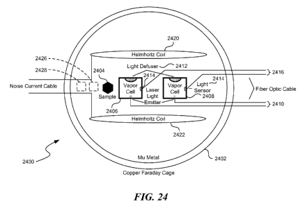
[0034] Figure 24 illustrates a diagram of a miniature atomic magnetometer-
based
molecular interrogation and data system (MIDS).
[0035] Figure 25 illustrates a block diagram of additional components for
use with the
miniature MIDS system of Figure 24.
[0036] Figure 26 illustrates a schematic diagram of a coil alignment system
for
pivoting and telescoping a noise coil.
[0037] Figure 27 illustrates a diagram of an optical magnetometer flow-thru
device for
molecular interrogation.
-4-
CA 02879008 2015-01-12
WO 2014/011940 PCT/US2013/050165
[0038] The headings provided herein are for convenience only and do not
necessarily
affect the scope or meaning of the claimed invention.
DETAILED DESCRIPTION
[0039] Described in detail below is a miniaturized detector for detecting
very low
amplitude signals to produce time-domain signals by recording a signal
produced by a
sample or compound in a shielded environment, while injecting a Gaussian white
noise
stimulus into the recording apparatus at a level that enhances the ability to
observe low-
frequency stochastic events produced by the compound. In commonly owned U.S.
Provisional applications 60/593,006 and 60/591,549, further noted belowõ the
transducing
signal was the actual compound time-domain signal of an effector compound.
[0040] The possibility of achieving effector-molecule functions by exposing
a target
system to characteristic effector-molecule signals, without the need for the
actual presence
of the effector agent, has a number of important and intriguing applications.
Instead of
treating an organism by the application of a drug, the same effect may be
achieved by
exposing the organism to drug-specific signals. In the field of
nanofabrication, it may now
be possible to catalyze or encourage self-assembly patterns by introducing in
the
assembly system, signals characteristic of multivalent effector molecules
capable of
promoting the desired pattern of self-assembly.
[0041] An apparatus and method for detecting the low level frequencies
produced by
biological samples through use of highly sensitive, yet miniaturized
magnetometers is
described in detail below. Apparatuses and methods for detecting, processing,
and
presenting low frequency electromagnetic emissions or signals of a sample of
interest are
provided where, in one embodiment, a known uniform white or Gaussian noise
signal is
introduced to the sample. The noise is configured to permit the
electromagnetic emissions
from the sample to be sufficiently detected by a signal detection system. Sets
of detected
signals are processed together to ensure repeatability and statistical
relevance. The
resulting emission pattern or spectrum can be displayed, stored, and/or
identified as a
particular substance.
-5-
CA 02879008 2015-01-12
WO 2014/011940 PCT/US2013/050165
[0042] Additional embodiments of the present invention describe signals for
use with
a transducing system for producing compound-specific electromagnetic waves
that can act
on target systems placed in the field of the waves and the corresponding
methods of
producing such signals. Other embodiments relate to generating and
distributing such
signals.
[0043] Various examples of the invention will now be described. The
following
description provides certain specific details for a thorough understanding and
enabling
description of these examples. One skilled in the relevant technology 'will
understand,
however, that the invention may be practiced without many of these details.
Likewise, one
skilled in the relevant technology will also understand that the invention may
include many
other obvious features not described in detail herein. Additionally, some well-
known
structures or functions may not be shown or described in detail below, to
avoid
unnecessarily obscuring the relevant descriptions of the various examples.
[0044] The terminology used below is to be interpreted in its broadest
reasonable
manner, even though it is being used in conjunction with a detailed
description of certain
specific examples of the invention. Indeed, certain terms may even be
emphasized below;
however, any terminology intended to be interpreted in any restricted manner
will be
overtly and specifically defined as such in this Detailed Description section.
[0045] The application is organized as follows, First some definitions are
provided.
Second, the inventors' earlier SQUID-based system is described to provide, in
part, an
understanding of basic signal acquisition. Third, methods of producing an
optimized time-
domain signal, and for forming transducing signals are discussed. Fourth,
certain
transduction apparatus and protocols are provided. Finally, the miniaturized
detector or
miniaturized molecular interrogation and data system is discussed in detail.
Those of
ordinary skill in the relevant art will recognize that aspects of the SQUID-
based system,
aspects of the methods for producing informing signals, and aspects of the
transduction
apparatus and protocols may individually or collectively be applied to the
miniaturized
detector to provide yet further embodiments of the invention that allow signal
acquisition
and use by the miniaturized detector.
-6-
CA 02879008 2015-01-12
WO 2014/011940 PCT/US2013/050165
l. Definitions
[0046] The terms below have the following definitions unless indicated
otherwise.
Such definitions, although brief, will help those skilled in the relevant art
to more fully
appreciate aspects of the invention based on the detailed description provided
herein.
Such definitions are further defined by the description of the invention as a
whole
(including the claims) and not simply by such definitions.
[0047] "Magnetic shielding" refers to shielding that decreases, inhibits or
prevents
passage of magnetic flux as a result of the magnetic permeability of the
shielding material.
[0048] "Electromagnetic shielding" refers to, e.g., standard Faraday
electromagnetic
shielding, or other methods to reduce passage of electromagnetic radiation.
[0049] "Time-domain signal" or 'time-series signal" refers to a signal with
transient
signal properties that change over time.
[0050] "Sample-source radiation" refers to magnetic flux or electromagnetic
flux
emissions resulting from molecular motion of a sample, such as the rotation of
a molecular
dipole in a magnetic field. Because sample source radiation is produced in the
presence
of an injected magnetic-field stimulus," it is also referred to as "sample
source radiation
superimposed on injected magnetic field stimulus."
[0051] "Stimulus magnetic field" or "Magnetic-field stimulus" refers to a
magnetic field
produced by injecting (applying) to magnetic coils surrounding a sample, one
of a number
of electromagnetic signals that may include (i) white noise, injected at
voltage level
calculated to produce, a selected magnetic field at the sample of between 0
and 1 G
(Gauss), (ii) a DC offset, injected at voltage level calculated to produce a
selected
magnetic field at the sample of between 0 and 1 G, and (iii) sweeps over a low-
frequency
range, injected successively over a sweep range between at least about 0-1kHz,
and at an
injected voltage calculated to produce a selected magnetic field at the sample
of between
0 and 1 G. The magnetic field produced at the sample may be readily calculated
using
known electromagnetic relationships, knowing the shape and number of windings
in the
injection coil, the voltage applied to coils, and the distance between the
injection coils and
the sample.
-7-
CA 02879008 2015-01-12
WO 2014/011940 PCT/US2013/050165
[0052]
A "selected stimulus magnetic-field condition" refers to a selected voltage
applied to a white noise or DC offset signal, or a selected sweep range, sweep
frequency
and voltage of an applied sweep stimulus magnetic field.
[0053]
"White noise" refers to random noise or a signal having simultaneous multiple
frequencies, e.g., white random noise or deterministic noise. Several
variations of white
noise and other noise may be utilized in the embodiments described in the
present
invention. For example, "Gaussian white noise" is white noise having a
Gaussian power
distribution. "Stationary Gaussian white noise" is random Gaussian white noise
that has
no predictable future components. "Structured noise" is white noise that may
contain a
logarithmic characteristic which shifts energy from one region of the spectrum
to another,
or it may be designed to provide a random time element while the amplitude
remains
constant. These two represent pink and uniform noise, as compared to truly
random noise
which has no predictable future component. "Uniform noise" means white noise
having a
rectangular distribution rather than a Gaussian distribution.
[0054]
"Frequency-domain spectrum" refers to a Fourier frequency plot of a time-
domain signal.
[0055]
"Spectral components" refers to singular or repeating qualities within a time-
domain signal that can be measured in the frequency, amplitude, and/or phase
domains.
Spectral components will typically refer to signals present in the frequency
domain.
[0056]
"Faraday cage" refers to an electromagnetic shielding configuration that
provides an electrical path to ground for unwanted electromagnetic radiation,
thereby
quieting an electromagnetic environment.
11. Apparatus for producing and processing time-domain signals
[0057]
Embodiments of the present invention provide a method and apparatus for
detecting extremely low-threshold molecular electromagnetic signals without
external
interference. They further provide for the output of those signals in a format
readily usable
by a wide variety of signal recording and processing equipment.
Accordingly,
embodiments of the present invention are directed to providing an apparatus
and method
for the repeatable detection and recording of low-threshold molecular
electromagnetic
-8-
CA 02879008 2015-01-12
WO 2014/011940 PCT/US2013/050165
signals. A magnetically shielded Faraday cage shields the sample material and
detection
apparatus from extraneous electromagnetic signals. Within the magnetically
shielded
Faraday cage, a coil injects uniform or white noise, a nonferrous tray holds
the sample,
and a gradiometer detects low-threshold molecular electromagnetic signals.
The
apparatus further includes a superconducting quantum interference device
("SQUID") and
a preamplifier.
[0058]
The apparatus is utilized by placing a sample within the magnetically shielded
Faraday cage in close proximity to the noise coil and gradiometer. White noise
is injected
through the noise coil and modulated until the molecular electromagnetic
signal is
enhanced through stochastic resonance. The enhanced molecular electromagnetic
signal,
shielded from external interference by the Faraday cage and the field
generated by the
noise coil, is then detected and measured by the gradiometer and SQUID. The
signal is
then amplified and transmitted to any appropriate recording or measuring
equipment.
[0059]
Figures 1-5 provide various views of the apparatus described in the previous
paragraphs. The apparatus illustrated provides one embodiment of the
invention, though
additional embodiments are described and contemplated within the scope of the
invention.
[0060]
Referring to Figure 1, an amplitude adjustable white noise generator 80 is
external to magnetic shielding cage 40, and is electrically connected to a
Helmholtz
transformer 60 (not shown) through filter 90 by electrical cable 82. The
Helmholtz coil, or
transformer 60, is illustrated and further described with reference to Figure
2. The white
noise generator 80 can generate nearly uniform noise across a frequency
spectrum from
zero to 100 kilohertz. In the illustrated embodiment, the filter 90 filters
out noise above 50
kilohertz, but other frequency ranges may be used. White noise generator 80 is
also
electrically connected to the other input of dual trace oscilloscope 160
through patch cord
164.
[0061]
A Flux Locked Loop 140 further amplifies and outputs a signal received from a
SQUID 120 via high-level output circuit 142 to an iMC-303 IMAGO SQUID
controller 150.
The SQUID is further described with reference to Figure 2 in the following
paragraphs.
The Flux-Locked Loop 140 is also connected via a model CC-60 six-meter fiber-
optic
composite connecting cable 144 to the SQUID controller 150. The fiber-optic
connecting
-9-
CA 02879008 2015-01-12
WO 2014/011940 PCT/US2013/050165
cable 144 and SQUID controller 150 are manufactured by Tristan Technologies,
Inc. The
controller 150 is mounted= externally to the magnetic shielding cage 40. The
fiber-optic
connecting cable 144 carriers control signals from the SQUID controller 150 to
the Flux
Locked Loop 140, further reducing the possibility of electromagnetic
interference with the
signal to be measured. It will be apparent to those skilled in the art that
other Flux-Locked
Loops, connecting cables, and Squid controllers can be used .
[0062] The SQUID controller 150 further comprises high resolution analog to
digital
converters 152, a standard GP-IB bus 154 to output digitalized signals, and
BNC
connectors 156 to output analog signals. In the illustrated embodiment, the
BNC
connectors are connected to a dual trace oscilloscope 160 through patch cord
162.
[0063] Referring now to Figure 2 a cross-sectional view of the elements
within the a
shielding structure 10 in Figure 1 is illustrated. The shielding structure 10
includes, in an
outer to inner direction, a conductive wire cage 16, which is a magnetic
shield, and inner
conductive wire cages 18 and 20, which provide electromagnetic shielding. In
another
embodiment, the outer magnetic shield 16 is formed of a solid aluminum plate
material
having an aluminum-nickel alloy coating, and the electromagnetic shielding is
provided by
two inner wall structures, each formed of solid aluminum.
[0064] As illustrated in Figure 2, the shielding structure, which can be a
Faraday cage
is open at the top, and includes side openings 12 and 14. The Faraday cage 10
is
further comprised of three copper mesh cages 16, 18 and 20, nestled in one
another.
Each of the copper mesh cages 16, 18 and 20 is electrically isolated from the
other cages
by dielectric barriers (not shown) between each cage.
[0065] Side openings 12 and 14 further comprise attenuation tubes 22 and 24
to
provide access to the interior of the Faraday cage 10 while isolating the
interior of the cage
from external sources of interference. Referring to Figure 3, attenuation tube
24 is
comprised of three copper mesh tubes 26, 28 and 30, nestled in one another.
The exterior
copper mesh cages 16, 18 and 20 are each electrically connected to one of the
copper
mesh tubes 26, 28 and 30, respectively. Attenuation tube 24 is further capped
with cap 32
and the cap may further include a hole 34. Attenuation tube 22 is similarly
comprised of
copper mesh tubes 26, 28 and 30, but does not include cap 32.
-10-
CA 02879008 2015-01-12
WO 2014/011940
PCT/US2013/050165
[0066]
A low-density nonferrous sample tray 50 is mounted in the interior of the
Faraday cage 10. The sample tray 50 is mounted so that it may be removed from
the
Faraday cage 10 through the attenuation tube 22 and side opening 12. Three
rods 52,
each of which is greater in length than the distance from the center vertical
axis of the
Faraday cage 10 to the outermost edge of the attenuation tube 22, are attached
to the
sample tray 50. The three rods 52 are adapted to conform to the interior curve
of the
attenuation tube 22, so that the sample tray 50 may be positioned in the
center of the
Faraday cage 10 by resting the rods in the attenuation tube. In the
illustrated embodiment,
the sample tray 50 and rods 52 are made of glass fiber epoxy. It will be
readily apparent to
those skilled in the art that the sample tray 50 and rods 52 may be made of
other
nonferrous materials, and the tray may be mounted in the Faraday cage 10 by
other
means, such as by a single rod.
[0067]
Mounted within the Faraday cage 10 and above the sample tray 50 is a
cryogenic dewar 100. In the disclosed embodiment, the dewar 100 is adapted to
fit within
the opening at the top of Faraday cage 10 and is a Model BMD-6 Liquid Helium
Dewar
manufactured by Tristan Technologies, Inc. The dewar 100 is constructed of a
glass-fiber
epoxy composite. A gradiometer 110 with a very narrow field of view is mounted
within the
dewar 100 in position so that its field of view encompasses the sample tray
50. In the
illustrated embodiment, the gradiometer 110 is a first order axial detection
coil, nominally 1
centimeter in diameter, with a 2 % balance, and is formed from a
superconductor. The
gradiometer can be any form of gradiometer excluding a planar gradiometer. The
gradiometer 110 is connected to the input coil of one low temperature direct
current
superconducting quantum interference device ("SQUID") 120.
In the disclosed
embodiment, the SQUID is a Model LSQ/20 LTS dc SQUID manufactured by Tristan
Technologies, Inc. It will be recognized by those skilled in the art that high
temperature or
alternating current SQUIDs can be used . In an alternative embodiment, the
SQUID 120
includes a noise suppression coil 124. The disclosed combination of
gradiometer 110 and
SQUID 120 have a sensitivity of 5 microTesla/4Hz when measuring magnetic
fields.
[0068]
The output of SQUID 120 is connected to a Model SP Cryogenic Cable 130
manufactured by Tristan Technologies, Inc. The Cryogenic Cable 130 is capable
of
-11-
.
CA 02879008 2015-01-12
WO 2014/011940 PCT/US2013/050165
withstanding the temperatures within and without the dewar 100 and transfers
the signal
from the SQUID 120 to Flux-Locked Loop 140, which is mounted externally to the
Faraday
cage 10 and dewar 100. The Flux-Locked Loop 140 in the disclosed embodiment is
an
iFL-301-L Flux Locked Loop manufactured by Tristan Technologies, Inc.
[0069] Referring still to Figure 2, a two-element Helmholtz transformer 60
is installed
to either side of the sample tray 50 when the sample tray is fully inserted
within the
Faraday cage 10. In the illustrated embodiment, the coil windings 62 and 64 of
the
Helmholtz transformer 60 are designed to operate in the direct current to 50
kilohertz
range, with a center frequency of 25 kilohertz and self-resonant frequency of
8.8
megahertz. In the illustrated embodiment, the coil windings 62 and 64 are
generally
rectangular in shape and are approximately 8 inches tall by 4 inches wide.
Other
Helmholtz coil shapes may be used but should be shaped and sized so that the
gradiometer 110 and sample tray 50 are positioned within the field produced by
the
Helmholtz coil. Each of coil windings 62 and 64 is mounted on one of two low-
density
nonferrous frames 66 and 68. The frames 66 and 68 are hingedly connected to
one
another and are supported by legs 70. Frames 66 and 68 are slidably attached
to legs 70
to permit vertical movement of the frames in relation to the lower portion of
dewar 100.
Movement of the frames permits adjustment of the coil windings 62 and 64 of
the
Helmholtz transformer 60 to vary the amplitude of white noise received at
gradiometer 110.
The legs 70 rest on or are epoxied onto the bottom of the Faraday cage 10. In
the
illustrated embodiment, the frames 66 and 68 and legs 70 are made of glass
fiber epoxy.
Other arrangements of transformers or coils may be used around the sample tray
50 .
[0070] Referring now to Figure 3, cable 82 is run through side opening 12,
attenuation
tube 24, and through cap 32 via hole 34. Cable 82 is a co-axial cable further
comprising a
twisted pair of copper conductors 84 surrounded by interior and exterior
magnetic shielding
86 and 88, respectively. In other embodiments, the conductors can be any
nonmagnetic
electrically conductive material, such as silver or gold. The interior and
exterior magnetic
shielding 86 and 88 terminates at cap 32, leaving the twisted pair 84 to span
the remaining
distance from the end cap to the Helmholtz transformer 60 shown in Figure 1.
The interior
magnetic shielding 86 is electrically connected to Faraday cage 16 through cap
32, while
-12-
CA 02879008 2015-01-12
WO 2014/011940 PCT/US2013/050165
the exterior magnetic shielding is electrically connected to the magnetically
shielded cage
40 shown in Figure '1.
[0071] Referring now to Figure 4, a cross-sectional view of the Faraday
cage and its
contents is further illustrated. The cage shows windings 62 of Helmholtz
transformer 60 in
relation to dewar 100 and Faraday cage 10.
[0072] Referring to Figures 1-4,an exemplary embodiment is now described. A
sample of the substance 200 to be measured is placed on the sample tray 50 and
the
sample tray is placed within the Faraday cage 10. In the first embodiment, the
white noise
generator 80 is used to inject white noise through the Helmholtz transformer
60. The noise
signal creates an induced voltage in the gradiometer 110. The induced voltage
in the
gradiometer 110 is then detected and amplified by the SQUID 120, the output
from the
SQUID is further amplified by the flux locked loop 140 and sent to the SQUID
controller
'150, and then sent to the dual trace oscilloscope 160. The dual trace
oscilloscope 160 is
also used to display the signal generated by white noise generator 80.
[0073] The white noise signal is adjusted by altering the output of the
white noise
generator 80 and by rotating the Helmholtz transformer 60 around the sample
200, shown
in Figure 2. Rotation of the Helmholtz transformer 60 about the axis of the
hinged
connection of frames 66 and 68 alters its phasing with respect to the
gradiometer '110.
Depending upon the desired phase alteration, the hinged connection of frames
66 and 68
permits windings 62 and 64 to remain parallel to one another while rotating
approximately
30 to 40 degrees around sample tray 50. The hinged connection also permits
windings 62
and 64 to rotate as much as approximately 60 degrees out of parallel, in order
to alter
signal phasing of the field generated by Helmholtz transformer 60 with respect
to
gradiometer 110.
[0074] The typical adjustment of phase will include this out-of-parallel
orientation,
although the other orientation may be preferred in certain circumstances, to
accommodate
an irregularly shaped sample 200, for example. Noise is applied and adjusted
until the
noise is 30 to 35 decibels above the molecular electromagnetic emissions
sought to be
detected. At this noise level, the noise takes on the characteristics of the
molecular
electromagnetic signal through the well-known phenomenon of stochastic
resonance. The
-13-
CA 02879008 2015-01-12
WO 2014/011940 PCT/US2013/050165
stochastic product sought is observed when the oscilloscope trace reflecting
the signal
detected by gradiometer 110 varies from the trace reflecting the signal
directly from white
noise generator 80. In alternative embodiments, the signal can be recorded and
or
processed by any commercially available equipment.
[0075] In an alternative embodiment, the method of detecting the molecular
electromagnetic signals further comprises injecting noise 180 out of phase
with the
original noise signal applied at the Helmholtz transformer 60 through the
noise
suppression coil 124 of the SQUID 120. The stochastic product sought can then
be
observed when the oscilloscope trace reflecting the signal detected by
gradiometer 110
becomes non-random.
[0076] Regardless of how the noise is injected and adjusted, the stochastic
product
can also be determined by observing when an increase in spectral peaks occurs.
The
spectral peaks can be observed as either a line plot on oscilloscope 160 or as
numerical
values, or by other well-known measuring devices.
[0077] Referring now to Figure 5, an alternative embodiment to the
molecular
electromagnetic emission detection and processing system of the above Figures
is shown.
A system 700 includes a detection unit 702 coupled to a processing unit 704.
Although the
processing unit 704 is shown external to the detection unit 702, at least a
part of the
processing unit can be located within the detection unit.
[0078] The detection unit 702, which is shown in a cross-sectional view in
Figure 5,
includes multiple components nested or concentric with each other. A sample
chamber or
Faraday cage 706 is nested within a metal cage 708. Each of the sample chamber
706
and the metal cage 708 can be comprised of aluminum material. The sample
chamber
706 can be maintained in a vacuum and may be temperature controlled to a
preset
temperature. The metal cage 708 is configured to function as a low pass
filter.
[0079] Between the sample chamber 706 and the metal cage 708 and encircling
the
sample chamber 706 are a set of parallel heating coils or elements 710. One or
more
temperature sensor 711 is also located proximate to the heating elements 710
and the
sample chamber 706. For example, four temperature sensors may be positioned at
-14-
CA 02879008 2015-01-12
WO 2014/011940 PCT/US2013/050165
different locations around the exterior of the sample chamber 706. The heating
elements
710 and the temperature sensor(s) 711 may be configured to maintain a certain
temperature inside the sample chamber 706.
[0080] A shield 712 encircles the metal cage 708. The shield 712 is
configured to
provide additional magnetic field shielding or isolation for the sample
chamber 706. The
shield 7'12 can be comprised of lead or other magnetic shielding materials.
The shield 712
is optional when sufficient shielding is provided by the sample chamber 706
and/or the
metal cage 708.
[0081] Surrounding the shield 712 is a cryogen layer 716 with G10
insulation. The
cryogen may be liquid helium. The cryogen layer 716 (also referred to as a
cryogenic
Dewar) is at an operating temperature of 4 degrees Kelvin. Surrounding the
cryogen layer
716 is an outer shield 7'18. The outer shield 718 is comprised of nickel alloy
and is
configured to be a magnetic shield. The total amount of magnetic shielding
provided by
the detection unit 702 is approximately -100 dB, -100 dB, and -120 dB along
the three
orthogonal planes of a Cartesian coordinate system.
[0082] The various elements described above are electrically isolated from
each other
by air gaps or dielectric barriers (not shown). It should also be understood
that the
elements are not shown to scale relative to each other for ease of
description.
[0083] A sample holder 720 can be manually or mechanically positioned
within the
sample chamber 706. The sample holder 720 may be lowered, raised, or removed
from
the top of the sample chamber 706. The sample holder 720 is comprised of a
material that
will not introduce Eddy currents and exhibits little or no inherent molecular
rotation. As an
example, the sample holder 720 can be comprised of high quality glass or
Pyrex.
[0084] The detection unit 702 is configured to handle solid, liquid, or gas
samples.
Various sample holders may be utilized in the detection unit 702. For example,
depending
on the size of the sample, a larger sample holder may be utilized. As another
example,
when the sample is reactive to air, the sample holder can be configured to
encapsulate or
form an airtight seal around the sample. In still another example, when the
sample is in a
gaseous state, the sample can be introduced inside the sample chamber 706
without the
-15-
CA 02879008 2015-01-12
WO 2014/011940 PCT/US2013/050165
sample holder 720. For such samples, the sample chamber 706 is held at a
vacuum. A
vacuum seal 721 at the top of the sample chamber 706 aids in maintaining a
vacuum
and/or accommodating the sample holder 720.
[0085] A sense coil 722 and a sense coil 724, also referred to as detection
coils, are
provided above and below the sample holder 720, respectively. The coil
windings of the
sense coils 722, 724 are configured to operate in the direct current (DC) to
approximately
50 kilohertz ( kHz) range, with a center frequency of 25 kHz and a self-
resonant frequency
of 8.8 MHz. The sense coils 722, 724 are in the second derivative form and are
configured
to achieve approximately 100% coupling. In one embodiment, the coils 722, 724
are
generally rectangular in shape and are held in place by G10 fasteners. The
coils 722, 724
function as a second derivative gradiometer.
[0086] Helmholtz coils 726 and 728 may be vertically positioned between the
shield
712 and the metal cage 708, as explained herein. Each of the coils 726 and 728
may be
raised or lowered independently of each other. The coils 726 and 728, also
referred to as
a white or Gaussian noise generation coils, are at room or ambient
temperature. The
noise generated by the coils 726, 728 is approximately 0.10 Gauss.
[0087] The degree of coupling between the emissions from the sample and the
coils
722, 724 may be changed by repositioning the sample holder 720 relative to the
coils 722,
724, or by repositioning one or both of the coils 726, 728 relative to the
sample holder 720.
[0088] The processing unit 704 is electrically coupled to the coils 722,
724, 726, and
728. The processing unit 704 specifies the white or Gaussian noise to be
injected by the
coils 726, 728 to the sample. The processing unit 104 also receives the
induced voltage at
the coils 722, 724 from the sample's electromagnetic emissions mixed with the
injected
Gaussian noise.
[0089] Referring to Figure 6, a processing unit employing aspects of the
invention
includes a sample tray 840 that permits a sample 842 to be inserted into, and
removed
from, a Faraday cage 844 and Helmholtz coil 746. A SQUID/gradiorneter detector
assembly 848 is positioned within a cryogenic dewar 850. A flux-locked loop
852 is
coupled between the SQUID/gradiometer detector assembly 848 and a SQUID
controller
-16-
CA 02879008 2015-01-12
WO 2014/011940 PCT/US2013/050165
854. The SQUID controller 854 may be a model iMC-303 iMAG multichannel
controller
provided by Tristan.
[0090] An analog noise generator 856 provides a noise signal (as noted
above) to a
phase lock loop 858. The x-axis output of the phase lock loop is provided to
the Helmholtz
coil 846, and may be attenuated, such as by 20 dB. The y-axis output of the
phase lock
loop is split by a signal splitter 860. One portion of the y-axis output is
input the noise
cancellation coil at the SQUID, which has a separate input for the
gradiometer. The other
portion of the y-axis signal is input oscilloscope 862, such as an
analog/digital oscilloscope
having Fourier functions like the Tektronix TDS 3000b (e.g., model 3032b).
That is, the x-
axis output of the phase lock loop drives the Helmholtz coil, and the y-axis
output, which is
in inverted form, is split to input the SQUID and the oscilloscope. Thus, the
phase lock
loop functions as a signal inverter. The oscilloscope trace is used to monitor
the analog
noise signal, for example, for determining when a sufficient level of noise
for producing
non-stationary spectral components is achieved. An analog tape recorder or
recording
device 864, coupled to the controller 854, records signals output from the
device, and is
preferably a wideband (e.g. 50 kHz) recorder. A PC controller 866 may be an MS
Windows based PC interfacing with the controller 854 via, for example, an RS
232 port.
[0091] In Figure 7, a block diagram of another embodiment of the processing
unit is
shown. A dual phase lock-in amplifier 202 is configured to provide a first
signal (e.g., "x" or
noise signal) to the coils 726, 728 and a second signal (e.g., "y" or noise
cancellation
signal) to a noise cancellation coil of a superconducting quantum interference
device
(SQUID) 206. The amplifier 202 is configured to lock without an external
reference and
may be a Perkins Elmer model 7265 DSP lock-in amplifier. This amplifier works
in a
"virtual mode," where it locks to an initial reference frequency, and then
removes the
reference frequency to allow it to run freely and lock to "noise."
[0092] An analog noise generator 200 is electrically coupled to the
amplifier 202. The
generator 200 is configured to generate or induce an analog white Gaussian
noise at the
coils 726, 728 via the amplifier 202. As an example, the generator 200 may be
a model
1380 manufactured by General Radio.
-17-
CA 02879008 2015-01-12
WO 2014/011940
PCT/US2013/050165
[0093] An impedance transformer 204 is electrically coupled
between the SQUID 206
and the amplifier 202. The impedance transformer 204 is configured to provide
impedance
matching between the SQUID 206 and amplifier 202.
[0094] The noise cancellation feature of the SQUID 206 can be
turned on or off.
When the noise cancellation feature is turned on, the SQUID 206 is capable of
canceling
or nullifying the injected noise component from the detected emissions. To
provide the
noise cancellation, the first signal to the coils 726, 728 is a noise signal
at 20 dB or 35 dB
above the molecular electromagnetic emissions sought to be detected. At this
level, the
injected noise takes on the characteristics of the molecular electromagnetic
signal through
stochastic resonance. The second signal to the SQUID 206 is a noise
cancellation signal
and is inverted from the first signal at an amplitude sufficient to null the
noise at the SQUID
output (e.g., 180 degrees out of phase with respect to the first signal).
[0095] The SQUID 206 is a low temperature direct element SQUID. As
an example,
the SQUID 206 may be a model LSQ/20 LTS dC SQUID manufactured by Tristan
Technologies, Inc. Alternatively, a high temperature or alternating current
SQUID can be
used. The coils 722, 724 (e.g., gradiometer) and the SQUID 206 (collectively
referred to
as the SQUID/gradiometer detector assembly) combined has a magnetic field
measuring
sensitivity of approximately 5 microTeslaNHz. The induced voltage in the coils
722, 724 is
detected and amplified by the SQUID 206. The output of the SQUID 206 is a
voltage
approximately in the range of 0.2-0.8 microVolts.
[0096] The output of the SQUID 206 is the input to a SQUID
controller 208. The
SQUID controller 208 is configured to control the operational state of the
SQUID 206 and
further condition the detected signal. As an example, the SQUID controller 208
may be an
iMC-303 iMAG multi-channel SQUID controller manufactured by Tristan
Technologies, Inc.
[0097] The output of the SQUID controller 208 is inputted to an
amplifier 210. The
amplifier 210 is configured to provide a gain in the range of 0-100 dB. A gain
of
= approximately 20 dB is provided when noise cancellation node is turned on
at the SQUID
206. A gain of approximately 50 dB is provided when the SQUID 206 is providing
no noise
cancellation.
-18-
CA 02879008 2015-01-12
WO 2014/011940 PCT/US2013/050165
[0098] The amplified signal is inputted to a recorder or storage device
212. The
recorder 212 is configured to convert the analog amplified signal to a digital
signal and
store the digital signal. In one embodiment, the recorder 212 stores 8600 data
points per
Hz and can handle 2.46 Mbits/sec. As an example, the recorder 212 may be a
Sony
digital audiotape (DAT) recorder. Using a DAT recorder, the raw signals or
data sets can
be sent to a third party for display or specific processing as desired.
[0099] A lowpass filter 214 filters the digitized data set from the
recorder 212. The
lowpass filter 214 is an analog filter and may be a Butterworth filter. The
cutoff frequency
is at approximately 50 kHz.
[00100] A bandpass filter 216 next filters the filtered data sets. The
bandpass filter 216
is configured to be a digital filter with a bandwidth between DC to 50 kHz.
The bandpass
filter 216 can be adjusted for different bandwidths.
[00101] The output of the bandpass filter 216 is the input to a Fourier
transformer
processor 218. The Fourier transform processor 218 is configured to convert
the data set,
which is in the time domain, to a data set in the frequency domain. The
Fourier transform
processor 218 performs a Fast Fourier Transform (FFT) type of transform.
[00102] The Fourier transformed data sets are the input to a correlation
and
comparison processor 220. The output of the recorder 212 is also an input to
the
processor 220. The processor 220 is configured to correlate the data set with
previously
recorded data sets, determine thresholds, and perform noise cancellation (when
no noise
cancellation is provided by the SQUID 206). The output of the processor 220 is
a final
data set representative of the spectrum of the sample's molecular low
frequency
electromagnetic emissions.
[00103] A user interface (UI) 222, such as a graphical user interface
(GUI), may also
be connected to at least the filter 216 and the processor 220 to specify
signal processing
parameters. The filter 216, processor 218, and the processor 220 can be
implemented as
hardware, software, or firmware. For example, the filter 216 and the processor
218 may
be implemented in one or more semiconductor chips. The processor 220 may be
software
implemented in a computing device.
-19-
CA 02879008 2015-01-12
WO 2014/011940 PCT/US2013/050165
[00104] This amplifier works in a "virtual mode," where it locks to an
initial reference
frequency, and then removes the reference frequency to allow it to run freely
and lock to
"noise." The analog noise generator (which is produced by General Radio, a
truly analog
noise generator) requires 20 dB and 45-dB attenuation for the Helmholtz and
noise
cancellation coil, respectively.
[00105] The Helmholtz coil may have a sweet spot of about one cubic inch
with a
balance of 11100th of a percent. In an alternative embodiments, the Helmholtz
coil may
move both vertically, rotationally (about the vertical access), and from a
parallel to spread
apart in a pie shape. In one embodiment, the SQUID, gradiometer, and driving
transformer (controller) have values of 1.8, 1.5 and 0.3 micro-Henrys,
respectively. The
Helmholtz coil may have a sensitivity of 0.5 Gauss per amp at the sweet spot.
[00106] Approximately 10 to 15 microvolts may be needed for a stochastic
response.
By injecting noise, the system has raised the sensitivity of the SQUID device.
The SQUID
device had a sensitivity of about 5 femtotesla without the noise. This system
has been
able to improve the sensitivity by 25 to 35 dB by injecting noise and using
this stochastic
resonance response, which amounts to nearly a 1,500% increase.
[00107] After receiving and recording signals from the system, a computer,
such as a
mainframe computer, supercomputer or high-performance computer does both pre
and
post processing, such by employing the Autosignal software product by Systat
Software of
Richmond CA, for the pre-processing, while Flexpro software product does the
post-
processing. Flexpro is a data (statistical) analysis software supplied by
Dewetron, Inc.
The following equations or options may be used in the Autosignal and Flexpro
products.
[00108] "A flow diagram of the signal detection and processing performed
by the
system 100 is shown in Figure 8. When a sample is of interest, at least four
signal
detections or data runs are performed: a first data run at a time ti without
the sample, a
second data run at a time t2 with the sample, a third data run at a time t3
with the sample,
and a fourth data run at a time t4 without the sample. Performing and
collecting data sets
from more than one data run increases accuracy of the final (e.g., correlated)
data set. In
the four data runs, the parameters and conditions of the system 100 are held
constant
(e.g., temperature, amount of amplification, position of the coils, the noise
signal, etc.).
-20-
CA 02879008 2015-01-12
WO 2014/011940 PCT/US2013/050165
[00109] At a block 300, the appropriate sample (or if it's a first or
fourth data run, no
sample), is placed in the system 100. A given sample, without injected noise,
emits
electromagnetic emissions in the DC-50 kHz range at an amplitude equal to or
less than
approximately 0.001 microTesla. To capture such low emissions, a white
Gaussian noise
is injected at a block 301.
[00110] At a block 302, the coils 722, 724 detect the induced voltage
representative of
the sample's emission and the injected noise. The induced voltage comprises a
continuous stream of voltage values (amplitude and phase) as a function of
time for the
duration of a data run. A data run can be 2-20 minutes in length and hence,
the data set
corresponding to the data run comprises 2-20 minutes of voltage values as a
function of
time.
[00111] At a block 304, the injected noise is cancelled as the induced
voltage is being
detected. This block is omitted when the noise cancellation feature of the
SQUID 206 is
turned off.
[00112] At a block 306, the voltage values of the data set are amplified by
20-50 dB,
depending on whether noise cancellation occurred at the block 304. At block
308, the
amplified data set undergoes analog to digital (A/D) conversion and is stored
in the
recorder 212. A digitized data set can comprise millions of rows of data.
[00113] After the acquired data set is stored, at a block 310 a check is
performed to
see whether at least four data runs for the sample have occurred (e.g., have
acquired at
least four data sets). If four data sets for a given sample have been
obtained, then
lowpass filtering occurs at a block 312. Otherwise, the next data run is
initiated (return to
the block 300).
[00114] After lowpass filtering (block 312) and bandpass filtering (at a
block 314) the
digitized data sets, the data sets are converted to ,the frequency domain at a
Fourier
transform block 316.
[00115] Next, at a block 318, like data sets are correlated with each other
at each data
point. For example, the first data set corresponding to the first data run
(e.g., a baseline or
ambient noise data run) and the fourth data set corresponding to the fourth
data run (e.g.,
-21-
CA 02879008 2015-01-12
WO 2014/011940 PCT/US2013/050165
another noise data run) are correlated to each other. If the amplitude value
of the first data
set at a given frequency is the same as the amplitude value of the fourth data
set at that
given frequency, then the correlation value or number for that given frequency
would be
1 Ø Alternatively, the range of correlation values may be set at between 0-
100. Such
correlation or comparison also occurs for the second and third data runs
(e.g., the sample
data runs). Because the acquired data sets are stored, they can be accessed at
a later
time as the remaining data runs are completed.
[00116] When the SQUID 206 provides no noise cancellation, then
predetermined
threshold levels are applied to each correlated data set to eliminate
statistically irrelevant
correlation values. A variety of threshold values may be used, depending on
the length of
the data runs (the longer the data runs, greater the accuracy of the acquired
data) and the
likely similarity of the sample's actual emission spectrum to other types of
samples. In
addition to the threshold levels, the correlations are averaged. Use of
thresholds and
averaging correlation results in the injected noise component becoming very
small in the
resulting correlated data set.
[00117] If noise cancellation is provided at the SQUID 206, then the use of
thresholds
and averaging correlations are not necessary.
[00118] Once the two sample data sets have been refined to a correlated
sample data
set and the two noise data sets have been refined to a correlated noise data
set, the
correlated noise data set is subtracted from the correlated sample data set.
The resulting
data set is the final data set (e.g., a data set representative of the
emission spectrum of the
sample) (block 320).
[00119] Since there can be 8600 data points per Hz and the final data set
can have
data points for a frequency range of DC-50 kHz, the final data set can
comprise several
hundred million rows of data. Each row of data can include the frequency,
amplitude,
phase, and a correlation value.
III. Methods of producing an optimized time-domain signal
[00120] It has been discovered that sample-dependent spectral features in a
low-
frequency time-domain signal obtained for a given sample can be optimized by
recording
-22-
CA 02879008 2015-01-12
WO 2014/011940 PCT/US2013/050165
time-domain signals for the sample over a range of noise levels. The range can
provide
power gain on the noise injected into the sample during signal recording. The
recorded
signals are then processed to reveal spectral signal features. The time domain
signal
having an optimal spectral-features score, as detailed below, is selected. The
selection of
optimized or near-optimized time-domain signals is useful because it has been
found, also
in accordance with the invention, that transducing a chemical or biological
system with an
optimized time-domain signal gives a stronger and more predictable response
than with a
non-optimized time-domain signal. In other words, selecting an optimized (or
near-
optimized) time-domain signal is useful in achieving reliable, detectable
sample effects
when a target system is transduced by the sample signal.
[00121] In general, the range of injected noise levels over which time-
domain signals
are typically recorded between about 0 to 1 volt, typically, or alternatively,
the noise
injected is preferably between about 30 to 35 decibels above the molecular
electromagnetic emissions sought to be detected, e.g., in the range 70-80
¨dbm. The
number of samples that are recorded, i.e., the number of noise-level intervals
over which
time-domain signals are recorded may vary from 10-100 or more. This variance
is typical
and occurs over sufficiently small intervals such that a good optimum signal
can be
identified. For example, the power gain of the noise generator level can be
varied over 50
20 mV intervals. As will be seen below, when the spectral-feature scores for
the signals
are plotted against level of injected noise, the plot shows a peak extending
over several
different noise levels when the noise-level increments are suitable small.
[00122] Embodiment of the present invention contemplate three different
methods for
calculating spectral-feature scores for the recorded time-domain signals.
These method
include (1) a histogram bin method, (2) generating an FFT of autocorrelated
signals, and
(3) averaging of FFTs, and each of these is detailed below.
[00123] Although not specifically described, it will be appreciated that
each method
may be carried out in a manual mode, where the user evaluates the spectra on
which a
spectral-feature score is based, makes the noise-level adjustment for the next
recording,
and determines when a peak score is reached, or it may be carried out in an
automated or
-23-
CA 02879008 2015-01-12
WO 2014/011940 PCT/US2013/050165
semi-automated mode, in which the continuous incrementing of noise level
and/or the
evaluation of spectral-feature score, is performed by a computer-driven
program.
A. Histogram Method of Generating Spectral Information
[00124] Figure 9 is a high level data flow diagram in the histogram method
for
generating spectral information. Data acquired from the SQUID (box 2002) or
stored data
(box 2004) is saved as 16 bit WAV data (box 2006), and converted into double-
precision
floating point data (box 2008). The converted data may be saved (box 2010) or
displayed
as a raw waveform (box 2012). The converted data is then passed to the
algorithm
described below with respect to Figure 10, and indicated by the box 2014
labeled Fourier
Analysis. The histogram can be displayed at 2016. Alternatively, and as will
be described
below, the converted data may be passed to one of two additional al
[00125] With reference to Figure 10, the general flow of the histogram
algorithm is to
take a discrete sampled time-domain signal and use Fourier analysis to convert
it to a
frequency domain spectrum for further analysis. The time-domain signals are
acquired
from an ADC (analog/digital converter) and stored in the buffer indicated at
2102. This
sample is SampleDuration seconds long, and is sampled at SampleRate samples
per
second, thus providing SampleCount (SampleDuration * SampleRate) samples. The
FrequencyRange that can be recovered from the signal is defined as half the
SampleRate,
as defined by Nyquist. Thus, if a time-series signal is sampled at 10,000
samples per
second, the FrequencyRange will be 0 Hz to 5 kHz. One Fourier algorithm that
may be
used is a Radix 2 Real Fast Fourier Transform (RFFT), which has a selectable
frequency
domain resolution (FFTSize) of powers of two up to 216. An FFTSize of 8192 is
selected,
to provide provides enough resolution to have at least one spectrum bin per
Hertz as long
as the FrequencyRange stays at or below 8 kHz. The SampleDuration should be
long
enough such that SampleCount >(2*) FFTSize * 10 to ensure reliable results.
[00126] Since this FFT can only act on FFTSize samples at a time, the
program must
perform the FFT on the samples sequentially and average the results together
to get the
final spectrum. If one chooses to skip FFTSize samples for each FFT, a
statistical error of
1 / FFTSize A 0.5 is introduced. lf, however, one chooses to overlap the FFT
input by half
-24-
CA 02879008 2015-01-12
WO 2014/011940 PCT/US2013/050165
the FFTSize, this error is reduced to 1 / (0.81 * 2 * FFTSize) A 0.5. This
reduces the error
from 0.0110485435 to 0.0086805556. Additional information about errors and
correlation
analyses in general, consult Bendat & Piersol, "Engineering Applications of
Correlation
and Spectral Analysis", 1993.
[00127] Prior to performing the FFT on a given window, a data tapering
filter may be
applied to avoid spectral leakage due to sampling aliasing. This filter can be
chosen from
among Rectangular (no filter), Hamming, Henning, Bartlett, Blackman and
Blackman/Harris, as examples.
[00128] In an exemplary method, and as shown in box 2104, we have chosen
8192 for
the variable FFTSize, which will be the number of time-domain samples we
operate on at a
time, as well as the number of discrete frequencies output by the FFT. Note
that FFTSize
=8192 is the resolution, or number of bins in the range which is dictated by
the sampling
rate. The variable n, which dictates how many discrete RFFT's (Real FFT's)
performed, is
set by dividing the SampleCount by FFTSize * 2, the number of FFT bins. In
order for the
algorithm to generate sensible results, this number n should be at least 10 to
20 (although
other valves are possible), where more may be preferred to pick up weaker
signals. This
implies that for a given SampleRate and FFTSize, the SampleDuration must be
long
enough. A counter m, which counts from 0 to n, is initialized to zero, also as
shown in box
2104.
[00129] The program first establishes three buffers: buffer 2108 for
FFTSize histogram
bins, that will accumulate counts at each bin frequency; buffer 2110 for
average power at
each bin frequency, and a buffer 2112 containing the FFTSize copied samples
for each m.
[00130] The program initializes the histograms and arrays (box 2113) and
copies
FFTSize samples of the wave data into buffer 2112, at 2114, and performs an
RFFT on
the wave data (box 2115). The FFT is normalized so that the highest amplitude
is 1 (box
2116) and the average power for all FFTSize bins is determined from the
normalized
signal (box 2117). For each bin frequency, the normalized value from the FFT
at that
frequency is added to each bin in buffer 2108 (box 2118).
-25-
CA 02879008 2015-01-12
WO 2014/011940 PCT/US2013/050165
[00131]
In box 21'19 the program then looks at the power at each bin frequency,
relative to the average power calculated from above. If the power is within a
certain factor
epsilon (between 0 and '1) of the average power, then it is counted and the
corresponding
bin is incremented in the histogram buffer at 16. Otherwise it is discarded.
[00132]
Note that the average power it is comparing to is for this FFT instance only.
An enhanced, albeit slower algorithm might take two passes through the data
and compute
the average over all time before setting histogram levels. The comparison to
epsilon helps
to represent a power value that is significant enough for a frequency bin. Or
in broader
terms, the equation employing epsilon helps answer the question, "is there a
signal at this
frequency at this time?" If the answer is yes, it could due be one of two
things: (1)
stationary noise which is landing in this bin just this one time, or (2) a
real low level
periodic signal which will occur nearly every time. Thus, the histogram counts
will weed
out the noise hits, and enhance the low level signal hits. So, the averaging
and epsilon
factor allow one to select the smallest power level considered significant.
[00133]
Counter m is incremented at box 2120, and the above process is repeated for
each n set of VVAV data until m is equal to n (box 2121). At each cycle, the
average power
for each bin is added to the associated bin at 2118, and each histogram bin is
incremented
by one when the power amplitude condition at 2114 is met.
[00134]
When all n cycles of data have been considered, the average power in each
bin is determined by dividing the total accumulated average power in each bin
by n, the
total number of cycles (box 2122) and the results displayed (box 2123). Except
where
structured noise exists, e.g., DC = 0 or at multiples of 60 Hz, the average
power in each
bin will be some relatively low number.
[00135]
The relevant settings in this method are noise gain and the value of epsilon.
This value determines a power value that will be used to distinguish an event
over average
value. At a value of 1, no events will be detected, since power will never be
greater than
average power. As epsilon approaches zero, virtually every value will be
placed in a bin.
Between 0 and 1, and typically at a value that gives a number of bin counts
between about
20-50% of total bin counts for structured noise, epsilon will have a maximum
"spectral
-26-
CA 02879008 2015-01-12
WO 2014/011940 PCT/US2013/050165
character," meaning the stochastic resonance events will be most highly
favored over pure
noise.
[00136] Therefore, one can systematically increase the power gain on the
noise input,
e.g., in 50 mV increments between 0 and 1 V, and at each power setting, adjust
epsilon
until a histogram having well defined peaks is observed. Where, for example,
the sample
being processed represents a 20 second time interval, total processing time
for each
different power and epsilon will be about 25 seconds. When a well-defined
signal is
observed, either the power setting or epsilon or both can be refined until an
optimal
histogram, meaning one with the largest number of identifiable peaks, is
produced.
[00137] Under this algorithm, numerous bins may be filled and associated
histogram
rendered for low frequencies due to the general occurrence of noise (such as
environmental noise) at the low frequencies. Thus, the system may simply
ignore bins
below a given frequency (e.g., below 1 kHz), but still render sufficient bin
values at higher
frequencies to determine unique signal signatures between samples.
[00138] Alternatively, since a purpose of the epsilon variable is to
accommodate
different average power levels determined in each cycle, the program could
itself
automatically adjust epsilon using a predefined function relating average
power level to an
optimal value of epsilon.
[00139] Similarly, the program could compare peak heights at each power
setting, and
automatically adjust the noise power setting until optimal peak heights or
character is
observed in the histograms.
[00140] Although the value of epsilon may be a fixed value for all
frequencies, it is also
contemplated to employ a frequency-dependent value for epsilon, to adjust for
the higher
value average energies that may be observed at low frequencies, e.g., DC to
1,000. A
frequency-dependent epsilon factor could be determined, for example, by
averaging a
large number of low-frequency FFT regions, and determining a value of epsilon
that
"adjusts" average values to values comparable to those observed at higher
frequencies.
-27-
CA 02879008 2015-01-12
WO 2014/011940 PCT/US2013/050165
B. FFT of autocorrelated signals
[00141] In a second general method for determining spectral-feature scores,
time-
domain signals recorded at a selected noise are autocorrelated, and a fast
Fourier
transform (FFT) of the autocorrelated signal is used to generate a spectral-
features plot,
that is, a plot of the signal in the frequency domain. The FFTs are then used
to score the
number of spectral signals above an average noise level over a selected
frequency range,
e.g., DC to 1 kHz or DC to 8 kHz.
[00142] Figure 11 is a flow diagram of steps carried out in scoring
recorded time-
domain signals according to this second embodiment. Time-domain signals are
sampled,
digitized, and filtered as above (box 402), with the gain on the noise level
set to an initial
level, as at 404. A typical time domain signal for a sample compound 402 is
autocorrelated, at 408, using a standard autocorrelation algorithm, and the
FFT of the
autocorrelated function is generated, at 410, using a standard FFT algorithm.
[00143] An FFT plot is scored, at 412, by counting the number of spectral
peaks that
are statistically greater than the average noise observed in the
autocorrelated FFT and the
score is calculated at 414. This process is repeated, through steps 416 and
406, until a
peak score is recorded, that is, until the score for a given signal begins to
decline with
increasing noise gain. The peak score is recorded, at 418, and the program or
user
selects, from the file of time-domain signals at 422, the signal corresponding
to the peak
score (box 420).
[00144] As above, this embodiment may be carried out in a manual mode,
where the
user manually adjusts the noise setting in increments, analyzes (counts peaks)
from the
FFT spectral plots by hand, and uses the peak score to identify one or more
optimal time-
domain signals. Alternatively, one or more aspects of the steps can be
automated.
C. Averaged FFTs
[00145] In another embodiment for determining spectral-peak scores, an FFT
of many,
e.g., 10-20 time domain signals at each noise gain are averaged to produce a
spectral-
peaks plot, and scores are calculated as above.
-28-
CA 02879008 2015-01-12
WO 2014/011940 PCT/US2013/050165
[00146] Figure 12 is a flow diagram of steps carried out in scoring
recorded time-
domain signals according to this third embodiment. Time-domain signals are
sampled,
digitized, and filtered as above (box 424), with the gain on the noise level
set to an initial
level, as at 426. The program then generates a series of FFTs for the time
domain
signal(s) at each noise gain, at 428, and these plots are averaged at 430.
Using the
averaged FFT plot, scoring is done by counting the number of spectral peaks
that are
statistically greater than the average noise observed in the averaged FFT, as
at 432, 434.
This process is repeated, through the logic of 436 and 437, until a peak score
is recorded,
that is, until the score for a given signal begins to decline with increasing
noise gain. The
peak score is recorded, at 438, and the program or user selects, from the file
of time-
domain signals at 442, the signal corresponding to the peak score (box 440).
[00147] As above, this method may be carried out in a manual, semi-
automated, or
fully automated mode.
IV. Forming transducinq signals
[00148] Signals for various therapeutic uses, or for uses to otherwise
affect biological
systems, may be generated directly from processed time-domain signals. Signals
may
also be formed by constructing a signal having specific identified peak
frequencies. For
example, the system can take advantage of "signal-activity relationship" in
which molecular
signal features, e.g., characteristic peak frequencies of a compound, are
related to actual
chemical activity for the compound, analogous to structure-activity
relationships used in
traditional drug design. In one general application, signal-activity
relationships are used for
drug screening, following, in one example, the following method.
[00149] First, one or more compounds having desired activity are
identified, e.g.,
compounds capable of producing a desired response in a biological system. The
system
records a time-series signal for one of these compounds, and the wave form is
processed
or otherwise optimized to identify low-frequency peaks for that compound.
("Low-
frequency" in this case refers to peaks at or below 10 kHz.) The steps are
repeated for
each of a group of structurally related compounds. The structurally related
compounds
include those that are active (produce a desired response), and some that are
inactive for
-29-
CA 02879008 2015-01-12
WO 2014/011940 PCT/US2013/050165
the tested biological response. The spectral components of the two groups of
compounds
are compared to identify those spectral components that are uniquely
associated with
compound activity. For example, by analyzing forms from three active and two
inactive
compounds, one may identify those peaks in the signal found in the active
compounds,
and not in the inactive compounds, some of which are presumed to provide the
desired
biological response.
[00150] In like manner, the system may record and optimize any unknown
compound.
One may then analyze the resulting wave form with signals associated with
known
compounds to see if the unknown compound displays structural features
associated the
desired activity, and lack components associated with inactive components to
help identify
an active compound. Rules derivable from signal-structure relationships are
more
accessible and more predictive than rules derived from structure-activity
relationships,
since activity can be correlated with a relatively small number of peak
frequencies, rather
than a large number of structural variables. Thus, for use in drug design, one
can use the
presence or absence of certain peak frequencies to guide synthesis of drugs
with
improved pharmacokinetic or target activity. For example, if poor
pharmacokinetic
properties, or an undesired side effect, can be correlated with certain peak
frequencies,
novel compounds that lack or have reduced amplitudes in these frequencies
would be
suggested. As a result, the inventive system greatly simplifies the task of
formulating
useful drug-design rules, since the rules can be based on the relatively small
number of
peak frequencies.
[00151] A large database of spectral peak frequencies representing numerous
compounds would allow one to combine signal features to ''synthesize"
virtually any
drug or drug-combination property desired. By combining this database with a
chemical compound database, one may generate chemical structures that display
a desired peak-frequency set. This approach would be similar to current
computer-
assisted chemical-synthesis programs used to generate compound syntheses for
novel compounds of interest.
[00152] The system can employ numerous signal processing techniques, as
described
herein. For example, signals from two or more structurally-related compounds
can be
-30-
CA 02879008 2015-01-12
WO 2014/011940 PCT/US2013/050165
compared with one or more signals from a structurally-related, but inactive or
undesirable
compound to identify only the desired frequency components between the
signals. A
resulting signal may thus be constructed that includes only the desired peaks.
By then
generating a time-domain signal, that time-domain signal may be used for
therapeutic
purposes.
[00153]
Of course, a time-domain signal may be generated from the processed
frequency-domain signal of a single compound. For example, one may obtain the
frequency-domain signal for a desired sample, and produce a processed, desired
signal.
From the processed signal, a time-domain signal may be generated using known
techniques, which can then be employed for therapeutic or other uses as an
analog to the
compound itself.
[00154]
Figure 15A shows a typical time domain signal for a sample compound. In this
embodiment, the herbicide glyphosphate (RoundupR). The segment shown here is
taken
over the time interval 14.08 to 14.16 seconds.
The time-domain signal is then
autocorrelated using a standard autocorrelation algorithm, and the FFT of the
autocorrelated function is generated using a standard FFT algorithm.
[00155]
Using the FFT plot, such as illustrated in Figures 15B-15E, the plot is scored
by counting the number of spectral peaks that are statistically greater than
the average
noise observed in the autocorrelated FFT. This process is repeated until a
peak score is
recorded, that is, until the score for a given signal begins to decline with
increasing noise
gain. The peak score is recorded and the program or user selects, from the
file of time-
domain signals, the signal corresponding to the peak score.
[00156]
The series of autocorrelated FFT plots in Figures 15B-15E illustrate the
signal
analysis involved in this method. At a noise level of 70.9 ¨dbm (Figure 15B),
very few
peaks above background noise are observed (the highest spike represents 60
cycle
noise). At the optimum noise level of 74.8 ¨dbm (Figures 150 and 15D), which
represent
different recordings at the same noise level), numerous peaks statistically
greater than
average noise are observed throughout the frequency range of DC-8 kHz. Several
of
these peaks are less prominent or have disappeared at the higher noise gain of
78.3 ¨dbm
(Figure 15E).
-31-
CA 02879008 2015-01-12
WO 2014/011940 PCT/US2013/050165
[00157]
When the spectral-features scores for these signals are plotted as a function
of
noise setting, as shown in Figure 15F, the peak score in the noise setting of
about 75 ¨
dbm is observed. From this plot, the time-domain signals corresponding to one
or the
peak score is selected.
V. Transduction apparatus and protocols
[00158]
This section describes equipment and methodology for transducing a sample
with signals formed in accordance with aspects of the present invention, and
summarizes
experiments that demonstrate the response of various biological systems to
time-domain
signals of the present invention. The signals employed in these experiments,
which are
optimized time-domain signals formed in accordance with the method described
above
demonstrate the ability of signals in accordance with the invention to produce
a compound-
specific response in various biological systems.
[00159]
Figure 13 shows the layout of equipment for transducing a sample with an
agent-specific signal, in accordance with the invention.
The particular layout
accommodates five different samples, including three samples 444, 446, and 448
which
are held within transductions coils, and exposed to electromagnetic signals, a
sample 450
that serves as a control, and a sample 452 that serves as a chemical-induction
control.
The system of Figure 13 may be used for experimentation; if used for treating
a patient,
then some elements may be omitted, such as 448, 450, 452, etc.
[00160]
Transduction by an agent-specific signal is carried out by "playing" the
optimized agent-specific signal to the sample, using, where the signal is
recorded on a CD,
and is played on a CD recorded 454 through a preamplifier 456 and an audio
amplifier
458. This signal is supplied to the electromagnetic coils 444 and 446 through
separate
channels, as shown. In one embodiment, a Sony Model CDP CE375 CD Player is
used.
Channel 1 of the Player is connected to CD input 1 of Adcom Pre Amplifier
Model GFP
750. Channel 2 is connected to CD input 2 of Adcom Pre Amplifier Model GFP
750. CD's
are recorded to play identical signals from each channel. Alternatively, CD's
may be
recorded to play different signals from each channel. The coil in sample 448
is used
primarily to produce a white noise field as a control for experiments. For
example, a GR
-32-
CA 02879008 2015-01-12
WO 2014/011940 PCT/US2013/050165
analog noise generator provides a white Gaussian noise source for this coil.
Alternatively,
this coil can be used to play any prerecorded transduction signal via a second
Crown
amplifier.
[00161] Figure 14 shows sample transduction equipment 466 such as
represented by
any of samples 444, 446, and 448 in Figure 13. The equipment includes a
chamber 468
housing an electromagnet 470, and various probes for monitoring conditions
within the
chamber, e.g., temperature. The electromagnet sits on a base 474, and
includes,
conventionally a toroid ferromagnetic core and wire windings.
[00162] In one embodiment, the coils are engineered and manufactured by
American
Magnetics to provide uniform performance between coils. Each coil consists of
416 turns
of No.8 gauge (awg) square copper magnet wire, enamel coated, about a 2" air
core.
Each coil can produce approximately 1500 Gauss in the center at 10 Volts RMS
at 10
Amps RMS at 11 Hertz without exceeding a 15 degree Celsius rise in
temperature.
[00163] In operation, the sample, e.g., a human patient or a portion of the
patient's
body is place between the centrally between the coils. Thus, for example, the
coils may be
at opposite ends of a support bed, or on opposite sides of the bed, and on
opposite sides
of the patient's head. The coil is then activated, using signal generation
equipment like
that shown in Figure 13, for a predetermined therapeutic period, e.g., 1 to
several hours.
[00164] Figure 16 shows an example of a process for creating and applying
signals
under the inventive system. Under block 3102, the system receives and records
a time
domain signal from one or more samples, in a manner described above. Under
block
3104, the system generates a frequency domain signal, and then processes that
signal to
isolate the desired frequency components from undesired components. Under
block 3106,
the processed frequency domain signal is converted back into a time domain
signal. The
time domain signal may then be applied to a biological system to generate a
desired result,
under block 3108.
[00165] Referring to Figure 18, a method 3300 for modifying waveforms
begins in
block 3302 where the user obtains a starting waveform. For example, the user,
using
standard user interface techniques, selects and retrieves from data storage a
desired
-33-
CA 02879008 2015-01-12
WO 2014/011940 PCT/US2013/050165
waveform. Alternatively, the user may obtain a signal during "live"
interrogation of a
sample.
[00166] In block 3304, the user can combine the starting waveform with
another
waveform and if so desired, the user retrieves another waveform under block
3306. Of
course, the user can simply modify the starting waveform, if desired.
[00167] Under block 3308, the user modifies the starting waveform using any
of a
variety of techniques. Figure 19C shows an example where the user may simply
employ
standard user interface techniques, such as a mouse, to manipulate a pointer
3404 and
attenuate (or amplify) one or more frequency peaks in the starting waveform as
displayed
on a display device. For example, the user can simply click on a peak 3402 of
a displayed
portion of a waveform and, using the mouse, drag the peak down to attenuate
its
magnitude, as shown in Figure 19D.
[00168] Many other techniques may be employed. The user may simply select a
portion of a waveform, cut or copy it, and then paste it into the starting
waveform. For
example, referring to Figure 19A, the user may move the cursor about a portion
of a
waveform to select that portion of the waveform (shown as a dashed line box
3406). Once
selected, the user can select from one of several menu choices, such as to cut
that portion
from the waveform. Alternatively, once selected, the user may modify that
portion of the
waveform, such as by replacing it with a flat line, attenuate it, amplify it,
or perform various
other signal processing techniques.
[00169] The system may employ a library of waveforms that can be inserted
or
employed as desired by the user. The user can select a portion of the signal
and cause it
to filter out all peaks, thereby eliminating noise or undesired frequency
components in the
waveform. For example, Figure 19B shows an example of a waveform or filter
signal 3408
that may be stored in a library. By applying the signal 3408 to the waveform
of Figure 19A,
the system provides the resulting, processed waveform shown in Figure 19C.
[00170] The system may employ various mathematical techniques under block
3308 to
modify the starting waveform. For example, the starting waveform may be
combined using
a variety of mathematical techniques with one or more waveforms retrieved
under block
-34-
CA 02879008 2015-01-12
WO 2014/011940 PCT/US2013/050165
3306. Examples of such mathematical operations include:
addition, subtraction,
multiplication, convolution, cross-correlation, scaling of starting waveform
(SW) as a linear
or non-linear function of other waveforms, etc.
[00171]
Under block 3310, the routine 3300 queries the user regarding whether more
modifications to the starting waveform are desired. If so, the routine loops
back to again
perform under blocks 3304 through 3308. If not, then in block 3312, the user
may store
the resulting waveform. The stored waveform can then be used for future
modifications to
other starting waveforms, used for therapeutic effect, or a variety of other
reasons,
described herein.
[00172]
The following are some examples of additional techniques to shape a
waveform or set of waveforms in time series.
[00173]
Passive Filters: simple electronic filters are based on combinations of
resistors,
inductors and capacitors (or logical or programmed representations of same).
These filters
can be used to shape the waveform prior to recording, prior to processing, or
prior to
transduction. Various existing software packages or routines permit a user to
model the
responsive electronic filters. Such software routines may be readily employed
under the
inventive system to filter frequency domain waveforms using software modeled
versions of
such electronic filters.
[00174]
Active Filters: hardware or software filters can also be implemented using a
combination of passive components and amplifiers to create active filters.
These can have
high Q, and achieve resonance without the use of inductors. As with passive
filters,
software applications or routines exist for modeling the response of active
filters, and such
routines may be employed herein to modify waveforms using one or more active
filter
models. The inventive system may employ similar existing software routines to
implement
with the filters, processing and shaping described below.
[00175]
Digital Filters: a digital filter is an electronic filter (usually linear), in
discrete
time, that is normally implemented through digital electronic computation.
Digital filters are
typically either finite impulse response (FIR) or infinite impulse response
(IIR), though
there are others, such as a hybrid class of filters known as truncated
infinite impulse
-35-
CA 02879008 2015-01-12
WO 2014/011940 PCT/US2013/050165
response (TIIR) filters, which show finite impulse responses despite being
made from IIR
components.
[00176]
Digital Signal Processing: digital signal processing (e.g., executed as a
computer program) may simulate, e.g., comb filter having a tapped delay line.
The
program selects numbers from a string of digital values representing the
signal, at a
spacing that simulates a comb of a tapped delay line. These numbers are
multiplied by
constants, and added together to make the output of the filter. DSP allows for
multiple
pass bands or multiple band gaps, essentially allowing only a select set of
frequencies to
make it to an output stage.
[00177]
Wave Shaping: many well-known methods exist for shaping a waveform by
altering its rise time, sustain time, and decay time, or otherwise altering a
signal from, or to
a sine wave using full wave rectifiers or pulse width modulation (as
examples).
[00178]
All of the equipment described herein may be scaled to produce systems of
greater or lesser size or intensity for various applications. For example, if
the system to be
used to treat the human patient, then a system having a coil for generating
electromagnetic waves to be directed at a patient may be constructed. In one
example, a
bed having embedded therein round or square Helmholtz coils would receive the
time-
domain signal created from the processed frequency-domain signal. The patient
would
then receive the resulting electromagnetic wave to induce the desired
biological effect that
would otherwise be provided by, for example, ingesting the compound from which
the
signals was generated.
[00179]
A system for more targeted application of electromagnetic waves to a patient
is
of course possible. For example, one or more coils may be provided within a
small device
(such as a helmet, or handheld wand). This output device receives the time-
domain signal
produced from a desired frequency-domain signal, as noted above.
Resulting
electromagnetic waves can be directed to specific parts of a patient's body
via the output
device to produce a desired effect at a localized portion of the patient.
[00180]
Figure 17 shows an example of such a signal output device. A database 3202
stores signals from one or more compounds or samples. Alternatively, the
signals may be
-36-
CA 02879008 2015-01-12
WO 2014/011940 PCT/US2013/050165
unprocessed frequency- or time-domain signals generated as noted above. A
computer
3204 retrieves the signal (or signals) and provides it to a signal generator
3206. For
example, the computer retrieves a desired time-domain signal generated from a
processed
frequency domain signal that was created from a specific compound. The
computer then
provides the time domain signal to the signal generator 3206 to simply amplify
the signal.
Alternatively, the computer may retrieve processed frequency-domain signals
that the
signal generator converts into time-domain signals. The signals output from
the signal
generator 3206 may be modified by a signal modifier 3208. The signal modifier
may
perform additional amplification, filtering, and so forth. In an alternative
embodiment, the
computer 3204 performs the necessary signal generation modification, and thus
separate
circuitry for the signal generator 3206 and signal modifier 3208 may be
omitted.
Alternatively, the signal generator 3206 or signal modifier 3208 may be
eliminated.
[00181] The signal output device 3210 receives the signal and applies to a
patient
3212. As noted above, the signal output device may be a patient bed having
embedded
therein one or more coils to output electromagnetic waves. Alternatively, the
signal output
device 3210 can be a small, handheld device, a wearable device (such as an
article of
clothing containing a coil), and so forth.
[00182] The detector 702 obtains a signal from the sample 200, and that
signal is
processed by the processing unit 704 to produce a digital file 1501, such as a
.wav file.
That file may then be stored on a storage media 1502 and distributed or
transported to a
remote computer or other device. Any of the storage media noted above may be
employed for transporting signals or data files.
[00183] Aspects of the invention may be implemented in computer-executable
instructions, such as routines executed by a general-purpose computer, e.g., a
server
computer, wireless device or personal computer. Those skilled in the relevant
art will
appreciate that the invention can be practiced with other communications, data
processing,
or computer system configurations, including: Internet appliances, hand-held
devices
(including personal digital assistants (PDAs)), wearable computers, all manner
of cellular
or mobile phones, multi-processor systems, microprocessor-based or
programmable
consumer electronics, set-top boxes, network PCs, mini-computers, mainframe
computers,
-37-
CA 02879008 2015-01-12
WO 2014/011940 PCT/US2013/050165
and the like. Indeed, the terms "computer," "computing device," and similar
terms are
generally used interchangeably herein, and refer to any of the above devices
and systems,
as well as any data processor.
[00184] Aspects of the invention can be embodied in a special purpose
computer or
data processor that is specifically programmed, configured, or constructed to
perform one
or more of the computer-executable instructions explained in detail herein.
Aspects of the
invention can also be practiced in distributed computing environments where
tasks or
modules are performed by remote processing devices, which are linked through a
communications network, such as a Local Area Network (LAN), Wide Area Network
(WAN), or the Internet. In a distributed computing environment, program
modules may be
located in both local and remote memory storage devices.
[00185] Aspects of the invention, such as data files, may be stored or
distributed on
computer-readable media, including magnetically or optically readable computer
discs,
hard-wired or preprogrammed chips (e.g,, EEPROM semiconductor chips),
nanotechnology memory, biological memory, or other data storage media. Indeed,
computer implemented instructions, data structures, screen displays,
wave/signal files, and
other data under aspects of the invention may be distributed over the Internet
or over other
networks (including wireless networks), on a propagated signal on a
propagation medium
(e.g., an electromagnetic wave(s), a sound wave, etc.) over a period of time,
or they may
be provided on any analog or digital network (packet switched, circuit
switched, or other
scheme).
[00186] Alternatively, a transmitter 1504 within a signal collection,
processing and
transmission system 1500 transmits the file to a network 1506 (e.g., the
Internet), either via
an appropriate cable or hard-wire, or wirelessly. The file then may be
transmitted to a
computer 1512 via wired or wireless communication.
[00187] The file may be transmitted via the network to a remote location,
such as to a
transducer-receiver 1508. For example, a satellite network 1510 could be used
to transmit
the file to the transducer-receiver 1508.
-38-
CA 02879008 2015-01-12
WO 2014/011940 PCT/US2013/050165
[00188] The transducer-receiver 1508 could be a standard receiver for
receiving the
file, and include a transducer for transducing the file as an electromagnetic
signal to be
applied. In one embodiment, an implanted transducer-receiver is implanted into
a patient,
body or structure. Where the receiver component of the transducer-receiver
1508 is a
wireless receiver, then the transducer/receiver may receive the file
wirelessly via the
network (or satellite). In an alternative embodiment, a cell phone or mobile
device 1514
receives the file from the network and relays it to the transducer-receiver
via any known
wireless protocol, including short range wireless protocols such as Bluetooth,
any of the
IEEE802.11 protocols, etc.
[00189] A transducer-transceiver 1516, similar to the transducer-receiver
1508, has a
sensor 1518. Thus, the transducer-transceiver 1516 can not only similarly
receive the
transmitted file 1501 and transduce or apply it to a biological system, but
also obtain data
from the sensor 1518 and transmit that data back to the system 1500 (e.g., via
the
network).
[00190] According to Figure 21, an example of the transducer-receiver 1508
and
transducer-transceiver 1516 is provided which includes a power source 1530 for
providing
power to the device. A receiver-transceiver 1532 wired or wirelessly receives
the file 1501,
which may then be transduced or applied to a subject or sample via a
transducer 1534.
The file may be amplified by an amplifier 1536 and/or processed by a processor
1538.
Memory 1540 may store the file, or store data obtained from one or more
optional sensors
1518.
[00191] Figures 22 and 23 show transduction coils suitable for use in
aspects of the
invention. A transducer 494 in Figure 22 is a long solenoid, e.g., up to
several feet in
length. The field inside the solenoid is parallel to the axis of the solenoid
and constant
within the solenoid, going to zero outside the solenoid (in an approximation
of an infinitely
long solenoid). This finite length coil will have a substantially uniform
field only near its
center. Thus, by placing the sample or subject at the center of the coil, a
substantially
uniform magnetic field is created at the sample when the coil is energized
with the data file
1501 or MIDS signal.
-39-
CA 02879008 2015-01-12
WO 2014/011940 PCT/US2013/050165
[00192] By adding additional turns to the solenoid, such as additional
turns 500 in
solenoid 496 in Figure 23, additional field strength can be added at the ends
of the coil to
compensate for the fall off of the coil's magnetic fields at its ends.
[00193] With either or additional embodiments, the transduction coil may be
a small
implantable ferromagnetic coil, such as a vascular stent coil capable of
receiving
transducing signals either by electrodes attached to opposite ends of the
coil, by an
implantable system (like systems 1508, 1516) or by a remote, inductive system
in which an
electromagnet is placed near the body surface, against the patient's chest,
and signals are
transmitted inductively to the implanted coil.
[00194] As noted above, the system utilizes, as input, sound files obtained
in
stochastic resonance experiments and outputs frequencies, amplitudes, and
phases of the
content sinusoids. The system may employ a software routine, dubbed
"peakfinder,"
which in turn employ other software packages, such as Octave, and Pd, both of
which are
open-source and currently supported software platforms.
[00195] In addition, two environmental variables may be utilized. A first,
: PF_TMP,
specifies a temporary directory. A second, PF_BASE, specifies the location of
a
peakfinder folder. If PF_BASE is not supplied, a peakfinder.sh script attempts
to infer it
from its own invocation (assuming it is invoked as an absolute pathname). The
input file is
a stereo soundfile, assumed to be at a standard sample rate of 44100. The file
format may
be "wav," "au," or "aiff," in 16, 24, or 32 bit sample frames. The output file
is an ASCII file
specifying one sinusoid. For instance:
595 100.095749 0.095624 -0.091218 -0.028693
1487 250.155258 0.100177 0.040727 0.091524
[00196] Within the chart, the first field is the frequency in units of the
fundamental
analysis frequency, explained below, the second is the frequency in Hertz, the
third is the
peak magnitude of the sinusoid, in the input sound file native units, and the
fourth and fifth
are the amplitudes of the cosine and sine components of the sinusoid, the real
and
imaginary parts of the complex amplitude. The magnitude could, of course, be
inferred
-40-
CA 02879008 2015-01-12
WO 2014/011940 PCT/US2013/050165
from the real and imaginary components. The first field has no physical
meaning and is
intended for debugging purposes.
[00197] A technique for determining the amplitude and frequency of a single
sinusoid
in white noise is the Maximum Likelihood (ML) method, which has been extended
to
multiple sinusoids. This methods assume that the number of sinusoids is known
in
advance. The problem of finding an un-predetermined number of sinusoids is
harder to
treat mathematically but can be dealt with assuming that the sinusoids in
question are
adequately separated in frequency. Furthermore, a method is needed to
discriminate
between the presence and absence of a sinusoid.
[00198] The following analysis starts by considering a single sinusoid in
white noise
and progresses to the problems of multiple sinusoids and non-white (e.g.,
pink) noise.
Given a measured signal:
,
the (discrete-time) non-normalized Fourier transform is defined as:
N-1
FT {X[n]} (0=12gmk/Nx[n]
n=0
where k is the frequency in units of the fundamental frequency of the
analysis; 2/N
radians per sample. k need not be an integer; in practice extra values of k
can be filled in
as needed by zero-padding the signal. With the assumption that a single
sinusoid is
present, its most likely frequency is given by:
k = arg max FT tx[n]}(k) .
In other words, the best estimate is simply the value of k at which the
Fourier transform's
magnitude is the largest.
[00199] Next, the system determines if the estimated value of k corresponds
to a true
sinusoid or simply to random fluctuations. For this, the null hypothesis is
analyzed to
determine whether x[n] only contains white noise, with mean 0 and RMS
amplitude a, for
instance. The Fourier transform at each point k is a sum of N independent
random
-41-
CA 02879008 2015-01-12
WO 2014/011940 PCT/US2013/050165
variables, each equal to a sample x[n] times a complex number of unit
magnitude, so the
mean of each point of the Fourier transform is still zero, and the standard
deviation is
cs-VN . If the tail behavior of the individual noise samples is well behaved
(which it is for
Gaussian or Uniform noise, for instance) the resulting random variable FT
{x[n]}(k) will be
very nearly Gaussian for the values of N used (on the order of 106). So the
probability of
exceeding more than about 5a4N is very small.
[00200] On the other hand, a real-valued sinusoid with peak amplitude a and
frequency k (in the usual units of 27t/N) has a Fourier transform magnitude of
aN I 2 . To
get a magnitude of 50-VN , we only need a to be at least
10c o
, 0 _____________________________________
-4 AT 100
[00201] The method zero-pads the recorded sound file (between a factor of
two and
four, depending on the next power of two), and then reports peaks that exceed
this
amplitude threshold. A peak is defined as having greater magnitude for the
given value of
k than for its neighbors, and also having at least half again the magnitude of
the twenty
neighboring values of k (a band of roughly 207-c/N Hz, or 1/3 Hz. for a one-
minute
sample.)
[00202] If several sinusoids are present, provided their frequencies are
mutually
spaced more than about 20ic I N , the above method should resolve them
separately; each
sinusoid's influence on the calculated Fourier transform drops off as 2/ 37-ck
in amplitude at
k frequency units away from the peak.
[00203] To compensate for the non-white nature of noise signals, the
spectral
envelope of the measured signal is estimated. The noise can be assumed to be
locally
white in each narrow range of frequency (2021- /N as above), with the value of
0- varying
gently according to the frequency range chosen. Another issue is to determine
whether
the injected noise sample can be subtracted from the measured output of the
experiment.
In such a situation, with an easily measurable transfer function relating the
two, even if it is
-42-
CA 02879008 2015-01-12
WO 2014/011940 PCT/US2013/050165
nonlinear, an estimate of the transfer function is used to remove the bulk of
the noise from
the measured signal. This also increases the sensitivity of the method.
[00204] As can be seen from the description provided above, the system
allows a user
to create waveforms that may be used for therapeutic affect or otherwise
induce a reaction
in a biological system. Waveforms or spectral series generated from two or
more
compounds may be obtained. These two signals may then be combined to create a
single, combined signal having the properties of the two individual signals.
lf, for example,
the two original signals related to two different compounds having two
different therapeutic
properties, then the resulting, combined signal would have the combined
therapeutic
properties of the two compounds. The combined signal may then be manipulated
to
remove unwanted frequency component that have been found to be associated with
side
effects or negative reactions in a biological system.
[00205] Alternatively, if the two compounds produce similar responses in a
biological
system, then the two signals generated from those compounds can be compared to
identify common frequency components associated with generating the biological
effect. A
third signal may then be generated that includes only those frequency
components
associated with the biological effect. Thus, for example, signals from certain
pain reliever
drugs may be compared to identify common frequency components, and then
generate a
resulting signal for use in transmission, storage, or application to a
biological system.
Indeed, the system permits a new signal to be constructed that is not based
directly on
signals generated from one or more compounds. Instead, the system permits a
signal to
be generated having only peaks at desired frequencies, where such peaks have a
desired
result in a biological system. Thus, such a synthesized signal is independent
of existing
compounds.
VI. Miniaturized Molecular Interrogation Data System
[00206] A miniaturized MIDS can provide an alternative approach to the
SQUID-based
biodetection systems discussed in the previous sections. Such a MIDS includes
one or
more atomic magnetometers that have shown improved sensitivity to measure
changes in
ultra-low level magnetic fields produced from, e.g., biological samples.
Additionally,
-43-
CA 02879008 2015-01-12
WO 2014/011940 PCT/US2013/050165
utilizing the atomic magnetometers, or detectors, allows for a coil-free and
room
temperature based system, whereas, with the SQUID, cooling is required via
liquid helium
or nitrogen. The atomic detectors, however, require small magnetic fields in
order to
operate. Accordingly, application within the shielded apparatus discussed
above would
provide an environment with little to no external magnetic fields, thus
allowing for such
operation.
[00207]
Figure 24 shows a miniature atomic magnetometer-based MIDS detection
apparatus 2400 for use with biological samples. The device 2400 shown can be a
top
down view of a similar shielding configuration as shown in Figure 1 above, and
the
shielding 2402 is similar to room temperature shielding used in the systems
described
above. This shielding 2402 is utilized in conjunction with attenuation
achieved through the
use of gradiometers. Fiber optic cabling 2416 and 2410 enters through the
shielding via
attenuation tubes (e.g., elements 22 and 24 in Figures 2-4), which are cut to
specific
lengths in order to deliver specific frequencies to the atomic magnetometers.
The length of
the cables is dependent on the width of the attenuation tube and also the
frequencies to be
attenuated. The shielding 2402, attenuation tubes and other elements form a
shielding
structure that encloses the atomic magnetometers, sample, and Helmholtz coils.
The
shielding 2402 enclosure that includes the Faraday cage with a layer of Mu
metal on all
sides including top and bottom. The shielding enclosure forms a container that
may be
round or spherical, which may provide for greater attenuation, although other
shapes are
of course possible. As mentioned previously, the detector operates only with
small
magnetic fields and thus has a high sensitivity level. The thickness of
materials, and/or
the number of layers, in the shielding may be adjusted based on particular
applications of
the MIDS device. For example, for samples producing lower levels of magnetic
fields,
improved attenuation may be necessary to detect signals at those levels.
[00208]
In one embodiment, a sample 2404 may be lowered in from the top of the
shielding enclosure, between or adjacent to at least two miniaturized
magnetometers or
detectors 2406 and 2408. Alternatively the system could be built to allow
horizontal access
(e.g. like Figure 2 above), or be configured in any other way. (The terms
"detector" and
"magnetometers" are generally used interchangeably.) Importantly, the spacing
between
-44-
CA 02879008 2015-01-12
WO 2014/011940 PCT/US2013/050165
the sample and first detector 2406, and spacing between the first and second
detectors
2406 and 2408 may be selected to tune or optimize the system based on the
sample or
particular application to which the system is to be used. For example, with
detectors
having outside diameters of 2 cm allows for a first derivative gradiometer
with a spacing of
3.2 cm. Magnetic fields of the sample would be closely coupled to at least one
detector.
Two magnetometers connected together and separated a particular distance from
each
other can form a gradiometer. The two magnetometers are operated in opposition
and, if
sensing the same precise field, should cancel each other out (e.g., if no
field is present).
In practice, one of the magnetometers is closely coupled to the target source
(sample),
while the other is loosely coupled to the target source. Yet both
magnetometers are
equally sensing the background environment.
When the output of the target
magnetometer is summed with the inverted output of the background
magnetometer, the
background is cancelled, leaving only the target source (signal) to be
detected.
[00209]
While the detectors 2406 and 2408 are not coils, the ratios for separation
between detectors and coils would be roughly the same. The diameter of
gradiometer
coils and the distance between coils is adjusted or calculated to optimize the
signal-to-
noise ratio. These are called gradiometer baseline calculations and are
dependent on the
radius and area of each coil element (See, e.g., "Baseline Distance
Optimization for
SQUID Gradiometers; Alexander Garachtchenko, Applied Materials, Santa Clara
CA,
USA; Andrei Matlashov, Robert H. Kraus, Jr., Los Alamos National Laboratory,
Los
Alamos NM, USA"). For round coils a typical separation distance is 1.6 times
the radius
(for two identical coil elements). The distance increases as the
'environmental element'
diameter increases.
[00210]
A pair of Helmholtz coils 2420 and 2422 inject noise into the system, as
described above. The system uses stochastic resonance to elevate a sub
threshold signal
to detectable levels. A coil pair (coils 2420 and 2422) is used to produce
random noise for
the purpose of generating stochastic resonance between the injected noise and
a sub
threshold weak signal. The noise and signal sum in such a way that elevates
weak signal
components above a detection threshold, allowing for those signals to be
detected via
magnetometers with high sensitivity. Altering the gradient characteristics of
the field
-45-
CA 02879008 2015-01-12
WO 2014/011940 PCT/US2013/050165
influences how point charge might be disturbed around the target molecule in
solution, and
also affects the generation of current in the individual gradiometer coil
elements.
Changing the field characteristics impacts how the source field is produced
while also
changing the noise cancellation dynamics of the gradiometer. Both of these
parameters
have an impact on the signal to noise ratio of the detected signal. For
example, if the
noise is not sufficiently attenuated by the gradiometers, the low level signal
may not be
detected over a necessary threshold.
[00211] White noise can also be applied using a Helmholtz coil pair 2420,
2422 that
produces a noise field uniformly coupled to both magnetometer elements of the
gradiometer. White noise can be used to produce stochastic resonance,
elevating a sub
threshold signal to detectable levels. The stochastic product will be most
evident in the
first magnetometer, allowing for a further improvement in the signal to noise
ratio as the
injected noise is cancelled within the gradiometer.
[00212] Each of the two detectors 2406 and 2408 include corresponding fiber
optic
cables 2410 that direct infrared laser light into a vapor cell that contains
rubidium gas
atoms. Each cell may include a light diffuser 2412, and light sensors 2414
coupled to fiber
optic output cables 2416. An example of such a single magnetometer detector is
described
as a room temperature molecular magnetic field detector in U.S. Patent
Application
2011/0031969 A1, Atomic Magnetometer and Method of Sensing Magnetic Fields;
Kitching, et al, assigned to NIST. The detector uses laser light to heat a
material vapor
whose dynamics change in the presence of a magnetic field. The same, or a
second laser
light, is used to observe differences in absorption or light scattering as
magnetic fields alter
the dynamics of the vapor cloud. A separate vapor heater can also be used
rather than
using laser heating. Another example is a high-bandwidth optical magnetometer
described
by Ricardo Jimenez-Martinez, W. Clark Griffith, Svenja Knappe, John Kitching,
and Mark
Prouty in the Journal of the Optical Society of America B I OPTICAL PHYSICS
Vol. 29,
lss. 12 ¨ Dec. 1, 2012 pp: 3398-3403 (Editor: Henry van Driel, JOSA B, Vol.
29, Issue 12,
pp. 3398-3403 (2012)).
[00213] In general, the energetic dynamics of biologic systems allows for
perturbation
of the magnetic environment through the movement of charge as described by
Maxwell.
-46-
CA 02879008 2015-01-12
WO 2014/011940 PCT/US2013/050165
For example, protein dynamics force the movement of not only point charge
associated
with hinging events, but also the transfer of charge along charge pathways.
The ability to
observe the magnetic perturbations in the wake of charge movement can be
diagnostic of
materials under measurement.
[00214] The system uses two miniature magnetometers that may be in a first
or
second derivative configuration for noise reduction. A first order gradiometer
is two
detectors measuring the difference between the target source detector 2406
(proximate to
the sample) and an inverted background signal of the adjacent detector 2408
(i.e.,
adjacent to the other detector). If an additional set of detectors is added,
this measures a
second degree reading of the difference between a second target source
detector 2426
and an inverted background signal of a second adjacent detector 2428, making a
second
iteration of the reading. Again, in order for the results to be utilized as
first and second
order, the spacing between the magnetometers, the gradiometers (e.g., sets of
magnetometers) and the sample are equivalent. With a second order system, the
sample
signal variance, e.g., signal detected from the target source detector is more
accurate.
Thus, as an alternative configuration, the system may include a second
derivative
gradiometer to provide greater attenuation. This second derivative gradiometer
includes
two more magnetometers or detectors 2426 and 2428 oriented to the opposite
side of the
sample, in mirror image to the original pair (shown schematically in dashed
lines).
[00215] Change in light absorption or scattering from each magnetometer is
measured
by a photo sensor that outputs a voltage relational to the number of photons
detected.
Each magnetometer in the first or second derivative configuration senses the
environment
at the same instant, and the output of each magnetometer is in phase with the
other.
[00216] To accomplish noise reduction, one magnetometer is closely coupled
(via
magnetic fields) to a material under measurement (detector 2406), while a
second
magnetometer is placed at a distance from the sample (detector 2408). Because
the first
magnetometer is more closely coupled to the sample, any magnetic field related
to the
sample will have a greater inductive coupling to it than to the second
magnetometer.
However, each magnetometer will have equal coupling to fields in the
background
environment.
-47-
CA 02879008 2015-01-12
WO 2014/011940 PCT/US2013/050165
[00217] The phase of the output voltage of the second magnetometer
(detector 2408)
may be electronically inverted such that the phase of the second magnetometer
is 180
degrees out of phase with the first (detector 2406). The two voltage outputs
are then
summed, effectively canceling any voltage that was the product of
environmental noise.
The remaining voltage is relational to the sample and is stored as time series
data for
future processing.
[00218] Referring to Figure 25, an example of a system having a laser
emitter 2502
providing light to detectors 2406 and 2408. A noise generator 2504, such as an
General
Radio Model 1381 Random Noise Generator, provides a controlled amount of noise
to
Helmholtz coils 2420 and 2422 in order to inject noise in the form of a
magnetic field, into
the shielded system. A first light to voltage converter 2506 receives the
output from the
first detector 2406, while a second light to voltage converter 2508 receive
the output from
the second detector 2408. Outputs from the converters are summed by a voltage
summer
2510, whose output is then stored as a time series as noted above (shown as
block 2512).
The acquired data can be stored and processed using a variety of signal
analysis
techniques including spectral correlation, wavelets, Eigen analysis, and more,
and is
diagnostic of the material under study.
[00219] In general, entropy can be used to indirectly determine changes in
the signal to
noise ratio of a detected signal and coil alignment. A variety of mathematical
solutions can
be applied in real time or in post processing to determine entropy at the
output of the
detector. A typical method for measuring signal entropy is to observe how
signal energy is
distributed across a bandwidth. Energy that deviates from a Gaussian
distribution is
thought to have lower entropy than a purely random event.
[00220] A variety of spectral algorithms are useful in determining entropy
including
spectral auto correlations, Fourier analysis, wavelet analysis, and Eigen
analysis.
Adjustments to the orientation of the noise coil pair are made until a maximum
negative
deviation in entropy is observed at the output of the detector. If the
analysis is being
performed in real time adjustments can be made quickly and could be automated.
[00221] Adjustments can be made with respect to the noise coils. Figures
13A through
13F show examples of various coil arrangements or geometries to produce
differing
-48-
CA 02879008 2015-01-12
WO 2014/011940 PCT/US2013/050165
responses in system. Position-adjustable coils allows the coils to move from a
Helmholtz
configuration to other conformations. Each coil could be independently
repositioned as
indicated in the applicants other patents and applications to produce fields
with varying
gradients and vectors.
[00222] Figure 26 shows an example of a system 2600 for adjusting a coil
2602. The
coil 2602 maybe a Helmholtz coil, other coils discussed herein, or even the
detectors 2406
and 2408. A telescoping arm 2604 is positioned between a base or frame 2606
and a
gimbaled or ball joint 2608. The telescoping arm 2604 may include a servomotor
or other
electromechanical adjustment (not shown) to adjustably move the arm along one
axis. The
joint 2608 allows the coil 2602 to be rotated. Again another motor may be used
to
electromechanical move the coil about the joint.
[00223] Figure 27 illustrates an optical magnetometer flow through
configuration of a
gradiometer made from two atomic magnetometers and divided by an optical flow
tube in
one embodiment. In this configuration, the gas chambers, or cells 3106 and
3108, within
each magnetometer are uniformly optically pumped with a sample. The pump can
be a
parasitic pump coupled to an optical flow tube which extends between each
magnetometer. A sample is pumped by a parasitic pump 3102 between the
magnetometers 3106 and 3108 for a specified time interval over which
measurements are
taken from the light detectors located within each gas cell, similar to that
described with
reference to Figure 24. The cells of the magnetometers 3106 and 3108 can be
closely
spaced in order for optimal coupling to the flow tube 3104 and sample. New
samples can
be pumped after each time interval elapses. Further, stepper motors, not
shown, could
move the magnetometers 3106 and 3108 closer or further from the tube.
[00224] While not shown, the system may include a phase shifter,
appropriate
amplification, etc. The system may employ a DC offset, with the injected
noise.
= [00225] Many alternatives are, of course, possible. For example,
several detectors may
be arranged in a plane, such as in a cross arrangement. A tube or port may be
provided at
the center of the detectors, through which sample may be transported. Thus, a
material
may flow through the tube and be detected by the detectors, thereby permitting
a higher
rate detection of a stream of samples.
-49-
CA 02879008 2015-01-12
WO 2014/011940 PCT/US2013/050165
[00226] In another alternative, detectors may be placed in X, Y and Z axes,
to thereby
form a three-dimensional array of detectors. A sample may be placed in the
center of the
detectors and a detection made along the X, Y and Z axes. This alternative
allows a
sample to be analyzed in three dimensions, and thus the geometry or model of
the sample,
at a molecular level, maybe detected.
[00227] One benefit of the above embodiments is that the detectors are
effective at
room temperature, and thus a sample may be measured over a long period of
time, where
prior samples would typically be subjected to an extremely cold environment
and thus
could not withstand such cold for a long period of time. Prior systems
required a heater,
which can be avoided here. Many other advantages and benefits of the system
are of
course recognizable by those of ordinary skill in the art.
CONCLUSION
[00228] Further details regarding aspects of the system may be found in the
commonly
owned United States Patent Numbers 6,724,188, 6,995,558, 6,952,652, 7,081,747,
7,412,340, and 7,575,934, each of which is incorporated herein by reference in
its entirety.
[00229] Unless the context clearly requires otherwise, throughout the
description and
the claims, the words "comprise,'' "comprising," and the like are to be
construed in an
inclusive sense, as opposed to an exclusive or exhaustive sense; that is to
say, in the
sense of "including, but not limited to." The word "coupled", as generally
used herein,
refers to two or more elements that may be either directly connected, or
connected by way
of one or more intermediate elements. Additionally, the words "herein,"
"above," "below,"
and words of similar import, when used in this application, shall refer to
this application as
a whole and not to any particular portions of this application. Where the
context permits,
words in the above Detailed Description using the singular or plural number
may also
include the plural or singular number respectively. The word "or" in reference
to a list of
two or more items, that word covers all of the following interpretations of
the word: any of
the items in the list, all of the items in the list, and any combination of
the items in the list.
-50-
CA 02879008 2015-01-12
WO 2014/011940 PCT/US2013/050165
[00230] The above detailed description of embodiments of the invention is
not intended
to be exhaustive or to limit the invention to the precise form disclosed
above. While
specific embodiments of, and examples for, the invention are described above
for
illustrative purposes, various equivalent modifications are possible within
the scope of the
invention, as those skilled in the relevant art will recognize. For example,
while processes
or blocks are presented in a given order, alternative embodiments may perform
routines
having steps, or employ systems having blocks, in a different order, and some
processes
or blocks may be deleted, moved, added, subdivided, combined, and/or modified.
Each of
these processes or blocks may be implemented in a variety of different ways.
Also, while
processes or blocks are at times shown as being performed in series, these
processes or
blocks may instead be performed in parallel, or may be performed at different
times.
[00231] The teachings of the invention provided herein can be applied to
other
systems, not necessarily the system described above. The elements and acts of
the
various embodiments described above can be combined to provide further
embodiments.
[00232] All of the above patents and applications and other references,
including any
that may be listed in accompanying filing papers, are incorporated herein by
reference.
Aspects of the invention can be modified, if necessary, to employ the systems,
functions,
and concepts of the various references described above to provide yet further
embodiments of the invention.
[00233] These and other changes can be made to the invention in light of
the above
Detailed Description. While the above description details certain embodiments
of the
invention and describes the best mode contemplated, no matter how detailed the
above
appears in text, the invention can be practiced in many ways. Details of the
signal
processing system may vary considerably in its implementation details, while
still being
encompassed by the invention disclosed herein. As noted above, particular
terminology
used when describing certain features or aspects of the invention should not
be taken to
imply that the terminology is being redefined herein to be restricted to any
specific
characteristics, features, or aspects of the invention with which that
terminology is
associated. In general, the terms used in the following claims should not be
construed to
limit the invention to the specific embodiments disclosed in the
specification, unless the
-51-
CA 02879008 2015-01-12
WO 2014/011940 PCT/US2013/050165
above Detailed Description section explicitly defines such terms. Accordingly,
the actual
scope of the invention encompasses not only the disclosed embodiments, but
also all
equivalent ways of practicing or implementing the invention under the claims.
-52-