Note: Descriptions are shown in the official language in which they were submitted.
CA 02883288 2015-02-26
WO 2014/036300
PCT/US2013/057356
SYSTEM AND METHOD FOR DETERMINING A PROBABILITY OF WELL
SUCCESS USING STOCHASTIC INVERSION
CROSS REFERENCE TO RELATED APPLICATIONS
[0001] This application claims priority to U.S. Non-Provisional Application
No.
13/600,406 filed on August 31, 2012, the entire contents of which are herewith
incorporated
by reference.
FIELD
[0002] The present invention pertains in general to computation methods and
more
particularly to a computer system and computer implemented method for
determining a
probability of well success using stochastic inversion or determining a best
well location
from a plurality of possible well locations.
BACKGROUND
[0003] The field of decision analysis provides a framework for making
decisions
with uncertain outcomes and provides a value of information (VOI) metric. VOI
is a tool to
determine whether purchasing a new information source would improve a decision-
maker's
chances of taking the optimal action. In other words, VOI provides the
decision maker an
estimate of how a particular information source can improve the probability of
a successful
outcome. For example, a typical decision is to determine a successful well-
site given an
interpretation of available geophysical properties around that site. Various
geophysical
properties may be used including electrical resistivity via a magneto-
tellurics (MT) data
inversion (in the geothermal field), seismic, gravity, and electromagnetic (in
the oil and gas
context). The geophysical properties (e.g., seismic) would provide estimates,
through
inversion, of velocity, density and electrical conductivity.
[0004] In order to calculate a VOI, a posterior distribution is
calculated. However,
none of the conventional methods employ stochastic inversion to obtain the
posterior
distribution or probabilities. Conventional methods use statistics that are
acquired either
subjectively or by using non-physics based statistical methods that are
subjective in nature
CA 02883288 2015-02-26
WO 2014/036300
PCT/US2013/057356
and are not related to the physics of the rock formation leading to a
potentially erroneous
estimate of a probability of well success.
[0005] Therefore, there is a need for a method or methods that cure these
and other
deficiencies in the conventional methods to provide a decision-risk method by
moving from
subjective assessment of risks to a quantitative approach where parameters
calculated from
stochastic inversion replace a decision maker's conjectures.
SUMMARY
[0006] An aspect of the present invention is to provide a computer
implemented
method for determining a best well location from a plurality of possible well
locations. The
method includes drawing, using the computer, a plurality of earth models from
a posterior
distribution, wherein the posterior distribution is generated by stochastic
inversion of existing
data; calculating, by the computer, a well production at a plurality of
proposed well locations
within an earth model in the plurality of earth models using a relationship
between the well
production and earth parameters; calculating, by the computer, from the
plurality of earth
models, cost distributions using the relationship between well cost and the
earth parameters;
and calculating, by the computer, probability weighted values for the proposed
well locations
using probabilities from location dependent stochastic inversions as weights.
[0007] Another aspect of the present invention is to provide a computer
system for
determining a best well location from a plurality of possible well locations.
The computer
system includes a computer readable memory configured to store well locations
and existing
well data. The computer system further includes a processor in communication
with the
computer readable memory. The processor is configured to: (a) draw a plurality
of earth
models from a posterior distribution, wherein the posterior distribution is
generated by
stochastic inversion of existing data; (b) calculate the well production at a
plurality of
proposed well locations within an earth model in the plurality of earth models
using a
relationship between the well production and earth parameters; (c) calculate
from the
plurality of earth models, cost distributions using the relationship between
well cost and the
earth parameters; and (d) calculate probability weighted values for the
proposed well
locations using probabilities from location dependent stochastic inversions as
weights.
2
CA 02883288 2015-02-26
WO 2014/036300
PCT/US2013/057356
[0008] Although the various steps of the method according to one
embodiment of the
invention are described in the above paragraphs as occurring in a certain
order, the present
application is not bound by the order in which the various steps occur. In
fact, in alternative
embodiments, the various steps can be executed in an order different from the
order described
above or otherwise herein.
[0009] These and other objects, features, and characteristics of the
present invention,
as well as the methods of operation and functions of the related elements of
structure and the
combination of parts and economies of manufacture, will become more apparent
upon
consideration of the following description and the appended claims with
reference to the
accompanying drawings, all of which form a part of this specification, wherein
like reference
numerals designate corresponding parts in the various figures. It is to be
expressly
understood, however, that the drawings are for the purpose of illustration and
description
only and are not intended as a definition of the limits of the invention. As
used in the
specification and in the claims, the singular form of "a", "an", and "the"
include plural
referents unless the context clearly dictates otherwise.
BRIEF DESCRIPTION OF THE DRAWINGS
[0010] In the accompanying drawings:
[0011] FIG. 1 is an example of a depth section through a three
dimensional earth
model for a geothermal field derived by stochastic inversion of
Magnetotelluric data,
according to an embodiment of the present invention;
[0012] FIG. 2A shows an example of posterior distributions Pr(pld,/) of
the earth
parameter p (electrical resistivity in f2m) at one location x of the earth
shown in FIG. 1;
[0013] FIG. 2B shows an example of the posterior distributions Pr(pld,I)
of the
earth parameter thickness of layer h at one location x of the earth shown in
FIG. 1;
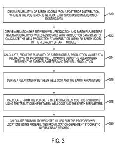
[0014] FIG. 3 is flow diagram of a method for determining a best well
location from
a number M o f possible well locations, according to an embodiment of the
present
invention;
3
CA 02883288 2015-02-26
WO 2014/036300
PCT/US2013/057356
[0015] FIG. 4 is a flow chart of the method for determining a Value of
Information
(VOI), according to an embodiment of the present invention;
[0016] FIG. 5A is a graph representing an example first earth model which
has a first
electrical resistivity across all x locations (x-coordinate) at a constant
depth, and an
associated first production;
[0017] FIG. 5B is a graph representing an example second earth model
having a
higher second electrical resistivity at the same depth as the first earth
model, and an
associated second production;
[0018] FIG. 5C is a graph showing a plot of a first production value as a
function
the x-coordinate and a plot of a second production value as a function of the
x-coordinate;
[0019] FIG. 6A is a graph of a first distribution of value (e.g., U.S.
dollars)
associated with the first electrical resistivity and depth and a second
distribution of value
associated with the constant second electrical resistivity and depth, at a
first position;
[0020] FIG. 6B is a graph of a first distribution of value associated
with the constant
first electrical resistivity and depth and a second distribution of value
associated with the
constant second electrical resistivity and depth, at a second position;
[0021] FIG. 6C shows a plot of the expected weighed value for each x
location
obtained for the first electrical resistivity, and a plot of the expected
weighed value for each x
location obtained for the second electrical resistivity;
[0022] FIG. 7A is a graph representing a first earth model where there
are plotted a
first electrical resistivity across all x locations, a first depth across all
x locations, and a first
production across all x locations;
[0023] FIG. 7B is a graph representing a second earth model where there
are plotted
a second electrical resistivity across all x locations, a second depth across
all x locations, and
a second production across all x locations;
4
CA 02883288 2015-02-26
WO 2014/036300
PCT/US2013/057356
[0024] FIG. 7C is a graph showing a plot of a first production value as a
function
the x-coordinate and a plot of a second production value as a function of the
x-coordinate;
[0025] FIG. 8A is a graph of a first distribution of value (e.g., U.S.
dollars)
associated with the first electrical resistivity and depth and a second
distribution of value
associated with the second electrical resistivity and depth, at a first
position;
[0026] FIG. 8B is a graph of a first distribution of value associated
with the first
electrical resistivity and depth and a second distribution of value associated
with the second
electrical resistivity and depth, at a second position;
[0027] FIG. 8C shows a plot of the expected weighed value for each x
location
obtained for the first electrical resistivity and a plot of the expected
weighed value for each x
location obtained for the second electrical resistivity;
[0028] FIG. 9 is a schematic diagram representing a computer system 50
for
implementing the method, according to an embodiment of the present invention.
DETAILED DESCRIPTION
[0029] In one embodiment, posterior analysis can be used to determine a
well
location with a highest possible outcome. That is posterior analysis can be
used to determine
which well-site x has a highest probability of success given an interpretation
of available
earth properties. Earth properties can be expressed as a vector of earth
parameters p. In the
following paragraphs, for illustration purposes, it may be referred to a
specific example of
earth property. However, as it can be appreciated, the vector p can include
any number of
earth parameters including, but not limited to, electrical resistivity,
velocity, permeability,
density, porosity, etc.
[0030] FIG. 1 is an example of a depth section through a three
dimensional earth
model for a geothermal field derived by stochastic inversion of
magnetotelluric data,
according to an embodiment of the present invention. In this case, the earth
parameters p are
layer electrical resistivity and depth to the top of a layer at three-
dimensional positions
defined by position vector x. At each location x in the model, the posterior
Pr(pl d,I)
defines a distribution for the earth parameter p at location x. The abscissa
axis represents the
CA 02883288 2015-02-26
WO 2014/036300
PCT/US2013/057356
position x. The ordinate axis represents the depth of z of a rock layer. The
term d represents
the geophysical data and the term I represents the prior information which can
be geological,
geophysical, or geochemical, etc., or any combination thereof Therefore, the
posterior
distribution Pr(p d, I) provides the posterior probability distribution of an
earth parameter p
conditional on evidence obtained from a geophysical data d.
[0031] FIG. 1 shows four different layers. The earth parameter (e.g., the
electrical
resistivity in f2m, for example) is represented by a graying-scale. A chart is
provided on the
right side of FIG. 1 providing a corresponding electrical resistivity to the
gray bars in FIG. 1.
As shown in FIG. 1, each layer has a variable electrical resistivity shown as
different gray-
scaled bars. Layer boundaries are shown by dotted lines. The values of
electrical resistivity
and layer depth plotted in FIG. 1 are median values of the posterior
distribution PrIpl
derived by a stochastic inversion of magnetotelluric data taken over a
geothermal field. In
this example, at each x position, there are four different electrical
resistivity values and three
depth values in the earth model.
[0032] FIG. 2A shows an example of posterior distributions Pr(pl d,I) of
the earth
parameter p (electrical resistivity in f2m) at one location x of the earth
shown in FIG. 1. At
each location x in the earth model there are four resistivities r 1, r2, r3
and T4. The abscissa
axis of the histogram represents the electrical resistivity and the ordinate
axis of the
histogram represents the frequency. A distribution of the electrical
resistivity of each layer of
the 4 layers is plotted. The median, standard deviation and mode values are
also provided.
For example, the first layer (layer 1) has a distribution centered around 70
f2m, corresponding
to electrical resistivity r 1, the second layer (layer 2) has a distribution
centered around 5 f2m,
corresponding to electrical resistivity r2, the third layer (layer 3) has a
distribution centered
around 40 f2m, corresponding to electrical resistivity r3, and the fourth
layer has a
distribution centered around 95 f2m, corresponding to electrical resistivity
r4.
[0033] FIG. 2B shows an example of the posterior distributions Pr(pl d,l)
of the
earth parameter thickness of layer h at one location x of the earth shown in
FIG. 1. The layer
thickness is plotted on the abscissa axis and the ordinate axis of the
histogram represents the
frequency. A distribution of the thickness of each of the 4 layers is plotted.
For example, the
6
CA 02883288 2015-02-26
WO 2014/036300
PCT/US2013/057356
first layer (layer 1) has a distribution centered around 300, corresponding to
thickness hl, the
second layer (layer 2) has a distribution centered around 1400, corresponding
to thickness h2,
the third layer (layer 3) has a distribution centered around 500,
corresponding to thickness h3.
[0034] The posterior distribution Pr(pl d ,I) can be used to generate any
number N
realizations of the earth by randomly drawing from the earth model parameter
distributions,
illustrated in FIGs. 2A and 2B.
[0035] FIG. 3 is a flow diagram of a method for determining a best well
location
from a number M o f possible well locations, according to an embodiment of the
present
invention. The method starts by drawing N earth models from the posterior
distribution Pr(pl d, I), where the posterior is generated by stochastic
inversion of existing
data, at S10. The posterior distribution Pr(pl d ,I) can be generated by any
stochastic
inversion technique. For example, in one embodiment, Markov Chain Monte Carlo
(MCMC)
techniques which evaluate the likelihood of any Earth model associated with
vector of
earth parameters p given some observed data d can be used. A description of
stochastic
inversion can be found in Trainor-Guitton & Hoversten (2011) "Stochastic
inversion for
electromagnetic geophysics: Practical challenges and improving convergence
efficiency,"
Geophysics 76, F373-F386. In general terms, stochastic inversion corresponds
to the
likelihood function f(dIpc)which describes the probability of candidate model
pc to occur
given the observed data d. In one embodiment, the likelihood function f(d pc)
can be
expressed by the following equation (1). Other definitions of likelihood
functions will result,
if different assumptions about the nature of the error model are made.
nData 1 id C(pc))2
f 0= 11 , ___ exp (1)
112-)371,2 2)3,2 di
[0036] Embedded in this exponential function is the misfit between the
observed
data d and the calculated data C. Therefore, Pr(pl d, I) represents a suite of
candidate
models and their respective probabilities generated through the likelihood of
equation (1).
[0037] As stated in the previous paragraphs p can be any parameterization
of the
earth (porosity, permeability, velocity, density, electrical resistivity,
etc.). However, for the
7
CA 02883288 2015-02-26
WO 2014/036300
PCT/US2013/057356
sake of illustration, we consider the case where p includes electrical
resistivity and depths to
layer tops. The data vector d could be any data that can be used to infer
earth model
parameters, for example, seismic, magnetotellurics, controlled source EM,
production data
from wells, geochemical, geological, etc. The symbol I represents the prior
information
about earth parameters p. The prior can be simple bounds on possible earth
model
parameters p. Alternatively, the prior can also b e a preferred set of the
model parameters or
distinct probability distributions of the earth model parameters p. At every
proposed well
location x, there is an associated model posterior, as illustrated for example
in FIGs .
2A and 2B. In addition, the probability of existence of any earth model
parameter p, can be
calculated using Pr(p d,I).
[0038] The method further includes deriving a relationship between earth
parameters
p and a well production q, given P existing wells associated with production
data, and
inputting the relationship, at S12. The relationship can be expressed by the
following
equation (2).
q(x) = f(p(x)) (2)
where x = 1, 2, ..., P, where P is the number of existing wells.
[0039] Equation (2) allows production q to be calculated at any position
x within an
earth model realization p. Production q is a quantitative scalar and can be in
many different
units depending on the specifics of the problem. For example, production q can
be expressed
in fluid volume, BTU per unit time, or expressed in revenue (currency such as
dollar amount).
The relationship expressed in Equation (2), can be derived from existing co-
located
production data and the Earth properties represented in p. For example,
electrical resistivity
models could be calibrated with the resulting production data that is observed
at that
location. Equation (2) can be a simple regression or a probabilistic
relationship based on
all data for a reservoir with no spatial dependence. However, if sufficient
production data
exists, f(p(x)) can be spatially dependent. The development of equation (2)
can be done
either in the same reservoir area where the decisions are to be made or
outside the area
where the decisions are to be made. Hence, the P wells used can be from
another field or
area as long as there is reason to believe they are representative of the
relationship that will
hold between p(x) and q in the area of interest.
8
CA 02883288 2015-02-26
WO 2014/036300
PCT/US2013/057356
[0040] The method further includes calculating, from N realizations of
the earth
model p, (i=1,..., N), production values at the M proposed well locations
using equation
(2), at S14.
[0041] The method further comprises deriving a relationship between well
cost and
earth parameters p, and inputting the relationship, at S16. This relationship
may originate
from work to date on the area under consideration or from a data base from
previous
experience or set of previous measurements. In a simplest case, the
relationship would only
depend on the depth parameters in p since to a first order approximation, the
cost of a well
cost(x) is directly related to the depth of the well. However, the
relationship can also take
into account the spatial variability of the hardness of the rock, for example.
The relationship
can be expressed as the function g(p) in equation (3) below. Similar to the
production
function, the cost function can be a simple regression or a probabilistic
distribution function.
cost(x) = g(p) (3)
[0042] The method also includes calculating cost distributions using
equation (3),
i.e., the relationship between well cost and the earth parameters, at S18. The
method also
includes calculating a production-cost ratio or value at well position x,
using the following
equation (4).
i
value q(x)
,(x)¨ (4)
cost, (x)
where x is equal to 1, 2, ..., M, where M is number of wells and x is the well
location.
[0043] The ratio or value is useful as it allows flexibility in the units
of
production and cost. The ratio is utilized for the risk-cost distribution for
decision analysis.
[0044] The method further includes calculating the probability-weighed
values or
risk-weighed values V(x) for all the considered M well locations, at S20. An
expected value
(e.g., average value) V(x) of any proposed well location x can be calculated
for all the
considered M well locations by using probabilities from location-dependent
stochastic
inversions Pr(p, do I) as weights. The probability weighed values can be
expressed by the
following equation (5).
9
CA 02883288 2015-02-26
WO 2014/036300
PCT/US2013/057356
V (X) = Pr(pi 1)valuei(x) (5)
where x = 1, 2, ..., M, M being the number of wells.
[0045] Therefore, calculating the probability weighted values V(x) for
the proposed
well locations x includes calculating a production-cost value value, (x) at a
given well
location x, multiplying the production-cost value value, (x) by the posterior
distribution Pr(pi do /) obtained from the stochastic inversion to obtain
weighed production-
cost values, and summing the weighed production-cost values over the plurality
of posterior
earth models (1...N).
[0046] The probability-weighed values V(x) at the M possible locations
can be
compared to each other to determine the most valuable location. The most
valuable location
corresponds to the location with the maximum value of V(x). This can be
expressed by the
following relationship (6).
Best well location x (among M well locations) = Max x V(x) (6)
[0047] In one embodiment, a number of model realizations N is chosen such
that the
mean and variance of V(x) asymptote to constant values as N increases.
[0048] An aspect of the present invention is to provide a method for
determining a
Value of Information (VOI) using posterior analysis. VOI provides a decision
maker an
estimate of how a particular information source can improve the probability of
a successful
outcome. FIG. 4 is a flow chart of the method for determining the VOI,
according to an
embodiment of the present invention. The method for determining VOI repeats
the steps
S10 through S20 described above with respect to FIG. 3 with the exception that
the initial
step S30 uses simulated data from synthetic earth models instead of using the
posterior
generated by stochastic inversion of existing data. In this embodiment, the
synthetic earth
models are drawn from one or more prior distribution(s) Pr(p1/). In this case
Pr(p1/)
represents the best estimate(s) of the geologic model based on all available
information. The
method provides the value of acquiring geophysical data.
CA 02883288 2015-02-26
WO 2014/036300
PCT/US2013/057356
[0049] The method for determining VOI includes creating or drawing L
prior earth
models pr" from the prior distribution Pr(p I) for M well locations
(x=1,2,..., M), and
generating, from each prior model, synthetic data, at S30.
[0050] The Drawing from the prior Pr(p I) does not require stochastic
inversion.
The drawing simply uses a Monte Carlo draw from the statistical representation
of the prior
uncertainty. For example, the statistical representation can be a histogram of
a particular
property (e.g., electrical resistivity and the layer boundaries).
Alternatively, the statistical
representation can be based on the generation of geostatistical realizations
using a
variogram or training image. The prior distribution differs from the posterior
distribution in
that the prior distribution is not informed by any geophysical, geochemical or
production data
d.
[0051] The method further includes drawing N Earth models p, from the
posterior
Pr(p l d,I) for M well locations ( x=1,2,..., M), at S32. In one embodiment,
the posterior
distribution is obtained through stochastic inversion. In one embodiment, this
is performed
by simulating the physics of the measurement for every prior synthetic earth
model
considered pT" , and then inverting the synthetic data for the earth
properties pi(x, j). In
one embodiment, the method includes drawing N posterior models from each prior
model.
In this notation of posterior earth properties pi(x, j), the index j denotes a
prior model
from which the posterior model originates.
[0052] The method further includes performing the same steps as in the
method
described with respect to FIG. 3. That is, perform the s am e steps for both
the prior
models to obtain q prior
) and the posterior models to obtain qi(x, j) . The index j represents
the prior earth model index and the index i represents the posterior earth
model index. The
index j varies from 1 to L, L being a number of synthetic prior earth models.
The index i
varies from 1 to N, N being the number of posterior earth models.
[0053] This includes deriving relationships between a well production q
and earth
parameters p for both the prior earth models and the posterior earth models,
given P existing
wells (one or more wells) associated with production data, and inputting the
relationships at
11
CA 02883288 2015-02-26
WO 2014/036300
PCT/US2013/057356
S34. The relationships can be expressed by the following equations (7) and
(8). Equations (7)
and (8) provide, respectively, the prior production and the posterior
production.
cor (x) f (pror (x)) (7)
qi(x, j)= f (p (x , j)) (8)
where x = 1, 2, ..., P, where P is the number of existing wells.
[0054] The method includes calculating, from the earth models, production
values at
the proposed well locations using the relationship between the earth
parameters and the well
production for both the prior earth models pr" and the posterior earth models
pi(x, j)
(where, i=1...N and j=1...L, at S36. Equations (7) and (8) allow production q
to be
calculated at any position x within an earth model realization p. The
relationship expressed
in Equations (7) and (8), can be derived from existing co-located production
data and the
Earth properties represented in p. For example, electrical resistivity models
could be
calibrated with the resulting production data that is observed at that
location. Equations (7)
and ( 8 ) can be regressions or probabilistic relationships based on all data
for a reservoir
without spatial dependence.
[0055] Similar to the method described above with respect to FIG. 3, the
present
method for determining VOI further comprises deriving a relationship between
prior well
cost and prior earth parameters pr" and a relationship between posterior well
cost and
posterior earth parameters p i(x, j), and inputting the relationships, at S38.
The relationships
may originate from work to date on the area under consideration or from a data
base from
previous experience or set of previous measurements. Similarly, in a simplest
case, the
relationships would only depend on the depth parameters in p since to a first
order
approximation, the cost of a well cost(x) (i.e., prior well cost and posterior
well cost)
is directly related to the depth of the well. However, the relationship can
also take into
account the spatial variability of the hardness of the rock, for example. The
relationship can
be expressed as the function g(p) in equations (9) and (10) below. Equations
(9) and (10)
provide, respectively, the prior well cost "cost7b0r (x)" and the posterior
well cost
"cost, (x, j)".
12
CA 02883288 2015-02-26
WO 2014/036300
PCT/US2013/057356
cost Pri" = u-1 '' prior \
(9)
./
cost, (x, j) = g(pi(x, j)) (10)
[0056] The method also includes calculating prior well cost distributions
and
posterior well cost distributions using equation (9) and (10), respectively,
at S40. The
method also includes calculating a prior value and a posterior value at well
position x, using
the following equation (11) or equation (12) at S42. Equation (11) and (12)
provide,
respectively, the value prior and the value posterior.
q prior (x) f (ppirior (x))
valueror (X) = ________________________ j = ___________ (11)
1 COSerwr g(p prior )
qi(x, j) f (p, (x, j))
value,(x, j)= (12)
cost, (x, j) g(pi(x, j))
where x is equal to 1, 2, ..., M, where M is number of wells and x is the well
location.
[0057] The ratio or value is useful as it allows flexibility in the units
of
production and cost. The ratio is utilized for the risk-cost distribution for
decision analysis.
[0058] The method for determining VOI further includes calculating a
difference or
a ratio between a weighted value posterior VP'ste'r and a weighted value prior
VP'r, for all
earth models at one location. In one embodiment, the weighted value prior
VPr'r for all earth
models at one location is calculated using the following equation (13).
vPrlOr (X) max[(1
EL Pr(plrr (x)11)valuer r (x)),0] (13)
>=
[0059] The two values within the max function represent the two decision
actions:
drilling a well or doing nothing. The value 0 at the end of equation (13)
signifies that no
action is taken (no drilling) therefore no cost nor value. The summation
represents the
weighted average (or expectation) of all the possible drawn values from the
prior. The
max signifies that the best outcome, given no further information, is the best
outcome on
average between the actions of doing nothing or drilling at that location x.
13
CA 02883288 2015-02-26
WO 2014/036300 PCT/US2013/057356
[0060] In one embodiment, the weighted value posterior VP'steri'r for all
earth models
at one location is also calculated using the following equation (14).
vPosterior (Jo = Epr(oor.,x.,
i)max[1
EN Pr(pi (x, j)1 d(x, j),I)valuei(x, j)),0] (14)
1=
J=1
[0061] Compared to equation (13) which provides VPrior, equation (14) has
an
additional expectation represented by the product in the inner summation. This
accounts for
the uncertainty of the information. The max operation is now inside the outer
summation.
This is because chronologically the decision maker will have the data d(x, j)
before the
decision is made.
[0062] The method further includes calculating a difference or a ratio
between the
weighted prior value and the weighted posterior value and calculating a sum
over the
plurality of well locations of the difference or the ratio between the
weighted prior value and
the weighted posterior value, at S46.
[0063] In one embodiment, the method includes calculating the VOI by
summing
over all possible M well locations, as expressed in the following equation
(15), at S44.
VO/ = z(vPosterior(x)¨ VPr r (X)) (15)
x=i
[0064] Although a difference operation between the weighted posterior
value
VP steri' and the weighted prior value VP6' is used inside the summation in
equation (15) to
calculate the VOI, it is also contemplated to calculate the VOI using a ratio
between the VP6'
and VP steri' as provided in the following equation (16), at S44.
M u Posterior r
VOI = E( p ")) (16)
x=1 v 101" (x)
[0065] Since value is a metric of success for a decision outcome, the VOI
equation
describes how an information source can increase the chances of making a
decision with a
higher valued outcome.
14
CA 02883288 2015-02-26
WO 2014/036300
PCT/US2013/057356
[0066] Table I summarizes the various mathematical notations used for
various
parameters and variables in the above description. As it can be appreciated,
although a
specific mathematical notation is used in the above paragraphs, other
mathematical notations
can also be used.
TABLE I
Vector of Earth Parameters
Vector of Geophysical Data
Prior Information (Geological,
Geophysical, Geochemical, etc)
Posterior Distribution Pr(pl d,I)
Prior Distribution Pr(p1/)
Posterior Earth model index
Total number of Posterior
Earth models
Well Location index
Number of Wells
Production
Cost of Production cost
Prior Earth model index
Total number of Prior Earth
models
[0067] In the following paragraphs, two examples are described using the
above
described methods. In the first example, two-dimensional earth models are
considered. FIG.
5A is a graph representing the first earth model p1 which has a first
electrical resistivity 50 of
500 ohm-m across all x locations (x-coordinate) at a constant depth 52 of 1500
m (on the y-
coordinate). The associated first production is also indicated in the graph at
54. In this
example, the first production is equal to 1000. In this example, the first
resistivity of 500
ohm-m results in a first production equal to 1000, as described in the above
paragraphs with
reference to equation (2).
CA 02883288 2015-02-26
WO 2014/036300
PCT/US2013/057356
[0068] FIG. 5B is a graph representing a second earth model p2 having a
higher
second electrical resistivity 51of 1500 ohm-m at the same depth 53 of 1500 m
as the first
earth model p1. The associated second production is also indicated in the
graph at 55. In
this example, the second production 55 is equal to 600. In this example, the
second
resistivity 51 of 1500 ohm-m results in a second production 55 equal to 600,
as described in
the above paragraphs with reference to equation (2).
[0069] FIG. 5C is a graph showing a plot of a first production value 56
as a function
the x-coordinate and a plot of a second production value 57 as a function of
the x-coordinate.
The first production 54 of 1000 (first model) provides a first production
value 56 of 300, and
the second production 55 of 600 (second model) provides a second production
value 57 of
250, as described above with respect to equation (4). Therefore, a lower
electrical resistivity
results in a higher production, and thus a higher production value.
[0070] However, the resistivity structure of the earth is unknown, and
the
information that is used to decipher the resistivity is uncertain. However,
the distributions of
possible electrical resistivity values at each location x or x-coordinate can
be obtained
through stochastic inversion. The distributions of possible electrical
resistivity values is
represented as Pr(pl d, I). As described in the above paragraphs with respect
to equations
(2), (3) and (4), the distributions of electrical resistivity can be
translated into distribution of
value (e.g., monetary value).
[0071] FIG. 6A is a graph of a first distribution 60 of value (e.g., U.S.
dollars)
associated with the constant first electrical resistivity 50 and depth 52 and
a second
distribution 61 of value associated with the constant second electrical
resistivity 51 and depth
53, at a first position (e.g., first position x at 1).
[0072] FIG. 6B is a graph of a first distribution 62 of value associated
with the
constant first electrical resistivity 50 and depth 52 and a second
distribution 63 of value
associated with the constant second electrical resistivity 51 and depth 53, at
a second position
(e.g., last position x at 361). These two distribution are drawn for 1500
samples (i=1500).
However, any number of samples can be implemented. FIG. 6C shows a plot of the
expected
weighed value 64 for each x location obtained for the first electrical
resistivity 50, and a plot
of the expected weighed value 66 for each x location obtained for the second
electrical
16
CA 02883288 2015-02-26
WO 2014/036300
PCT/US2013/057356
resistivity 51, using equation (5). The two plots 64 and 66 show that the
weighed values for
the second electrical resistivity 51 are less than the weighed values of the
first electrical
resistivity 50, across all x locations.
[0073] In a second example, two more complicated earth models are
considered. In
these earth models, both the depths of the earth layers and electrical
resistivities vary across
the x locations.
[0074] FIG. 7A is a graph representing a first earth model p1where there
are plotted
a first electrical resistivity 70 across all x locations (x-coordinate), a
first depth 72 across all x
locations, and a first production 74 across all x locations. The first
production 74 is obtained
using equation (2) described in the above paragraphs
[0075] FIG. 7B is a graph representing a second earth model p2 where
there are
plotted a second electrical resistivity 71 across all x locations (x-
coordinate), a second depth
73 across all x locations, and a second production 75 across all x locations.
The second
production 75 is also obtained using equation (2) described in the above
paragraphs.
[0076] As it can be noted in FIG. 7A, the curve of the first electrical
resistivity 70
has a peak or maximum of at around the center x location. On the other hand,
as can be noted
in FIG. 7B, the curve of the second electrical resistivity 71 has a trough or
minimum of at
around the center x location.
[0077] FIG. 7C is a graph showing a plot of a first production value 76
as a function
the x-coordinate and a plot of a second production value 77 as a function of
the x-coordinate.
The first production value 76 is obtained using the first earth model's first
depth 72 and first
electrical resistivity70 and the second production value 77 is obtained using
the second earth
model's second depth 73 and second electrical resistivity 71, as explained in
detail with
respect to equations (3) and (4) which express the dependence of a cost of
producing a
resource as a function of a location.
[0078] As stated above, the resistivity structure of the earth is
unknown, and the
information that is used to decipher the electrical resistivity is uncertain.
However, through
stochastic inversion, distributions of possible resistivity values at each
location x or x-
coordinate can be obtained. The distributions of possible resistivity values
is represented as
17
CA 02883288 2015-02-26
WO 2014/036300
PCT/US2013/057356
Pr(pl d,I). As described in the above paragraphs with respect to equations
(2), (3) and (4),
the distributions of resistivity can be translated into distributions of
value.
[0079] FIG. 8A is a graph of a first distribution 80 of value (e.g., U.S.
dollars)
associated with the first electrical resistivity 70 and depth 72 and a second
distribution 81 of
value associated with the second electrical resistivity 71 and depth 73, at a
first position (e.g.,
first position x at 1). FIG. 8A shows that electrical resistivity displays a
relatively smaller
variability as the distribution of value associated with the first electrical
resistivity and the
distribution of value associated with the second electrical resistivity
present maxima at almost
the same value (around approximately 300). In addition, it can be noted that
the distribution
of value is somewhat broader in the case of the first electrical resistivity
but the two
distributions have generally the same shape.
[0080] FIG. 8B is a graph of a first distribution 82 of value associated
with the first
electrical resistivity 70 and depth 72 and a second distribution 83 of value
associated with the
second electrical resistivity 71 and depth 73, at a second position (e.g.,
last position x at 361).
FIG. 8B shows that the electrical resistivity displays a relatively higher
variability as the
distribution of value associated with the first electrical resistivity and the
distribution of value
associated with the second electrical resistivity present maxima at different
values,
respectively 150 and about 350. In addition, it can be noted that the
distribution of value is
broader in the case of the first electrical resistivity and the general shape
of the first and
second value distributions are different.
[0081] FIG. 8C shows a plot of the expected weighed value 84 for each x
location
obtained for the first electrical resistivity 70 and a plot of the expected
weighed value 86 for
each x location obtained for the second electrical resistivity 71, using
equation (5). The two
plots 84 and 86 show that the expected weighed value for the second electrical
resistivity is
less than the expected weighed value of the first electrical resistivity at
around the mid-
section of x-coordinated. However, at small x-locations (between about 0 and
about 40), the
expected weighed value for the second electrical resistivity becomes greater
than the
expected weighed value of the first electrical resistivity and at higher x-
locations (between
about 340 and about 360), the expected weighed value for the second electrical
resistivity
approaches the expected weighed value of the first electrical resistivity.
18
CA 02883288 2015-02-26
WO 2014/036300
PCT/US2013/057356
[0082] In one embodiment, the method or methods described above can be
implemented as a series of instructions which can be executed by a computer.
As it can be
appreciated, the term "computer" is used herein to encompass any type of
computing system
or device including a personal computer (e.g., a desktop computer, a laptop
computer, or any
other handheld computing device), or a mainframe computer (e.g., an IBM
mainframe), or a
supercomputer (e.g., a CRAY computer), or a plurality of networked computers
in a
distributed computing environment.
[0083] For example, the method(s) may be implemented as a software
program
application which can be stored in a computer readable medium such as hard
disks,
CDROMs, optical disks, DVDs, magnetic optical disks, RAMs, EPROMs, EEPROMs,
magnetic or optical cards, flash cards (e.g., a USB flash card), PCMCIA memory
cards, smart
cards, or other media
[0084] Alternatively, a portion or the whole software program product can
be
downloaded from a remote computer or server via a network such as the
internet, an ATM
network, a wide area network (WAN) or a local area network.
[0085] Alternatively, instead or in addition to implementing the method
as computer
program product(s) (e.g., as software products) embodied in a computer, the
method can be
implemented as hardware in which for example an application specific
integrated circuit
(ASIC) can be designed to implement the method.
[0086] FIG. 9 is a schematic diagram representing a computer system 90
for
implementing the method, according to an embodiment of the present invention.
As shown
in FIG. 9, computer system 90 comprises a processor (e.g., one or more
processors) 92 and a
memory 94 in communication with the processor 92. The computer system 90 may
further
include an input device 96 for inputting data (such as keyboard, a mouse or
the like) and an
output device 98 such as a display device for displaying results of the
computation.
[0087] As can be appreciated from the above description, the computer
readable
memory can be configured to store well locations and existing well data. The
computer
processor can be configured to: (a) draw a plurality of earth models from a
posterior
19
CA 02883288 2015-02-26
WO 2014/036300
PCT/US2013/057356
distribution, wherein the posterior distribution is generated by stochastic
inversion of existing
data; (b) calculate the well production at a plurality of proposed well
locations within an earth
model in the plurality of earth models using a relationship between the well
production and
earth parameters; (c) calculate from the plurality of earth models, cost
distributions using the
relationship between well cost and the earth parameters; and (d) calculate
probability
weighted values for the proposed well locations using probabilities from
location dependent
stochastic inversions as weights.
[0088] As can be further appreciated from the above description, the
computer
readable memory can be configured to store well locations and existing well
data. The
computer processor can be configured to: (a) draw a plurality of synthetic
prior earth models
from one or more prior distributions for a plurality of well locations and
generate from each
prior distribution synthetic data; (b) draw a plurality of posterior earth
models from a
posterior distribution for the plurality of well locations, wherein the
posterior distribution is
generated through stochastic inversion and the plurality of posterior models
are drawn from
each of the plurality of prior earth models; (c) calculate, from the plurality
of prior earth
models and posterior earth models, the well production at a plurality of
proposed well
locations using a relationship between the earth parameters and the well
production for both
the prior earth models and the posterior earth models; (d) calculate the prior
well cost using a
relationship between the prior well cost and the earth parameters and
calculate a posterior
well cost using a relationship between the posterior well cost and the earth
parameters; (e)
calculate a value prior using the prior cost and the prior production and
calculate a value
posterior using the posterior cost and the posterior production; (f) calculate
a weighted prior
value and calculate a weighted posterior value using, respectively, the value
prior and the
value posterior; and (g) calculate a difference or a ratio between the
weighted value prior and
the weighted value posterior and calculate a sum over a plurality of well
locations of the
difference or the ratio to obtain the value of information.
[0089] Although the invention has been described in detail for the
purpose of
illustration based on what is currently considered to be the most practical
and preferred
embodiments, it is to be understood that such detail is solely for that
purpose and that the
invention is not limited to the disclosed embodiments, but, on the contrary,
is intended to
cover modifications and equivalent arrangements that are within the spirit and
scope of the
CA 02883288 2015-02-26
WO 2014/036300
PCT/US2013/057356
appended claims. For example, it is to be understood that the present
invention contemplates
that, to the extent possible, one or more features of any embodiment can be
combined with
one or more features of any other embodiment.
[0090] Furthermore, since numerous modifications and changes will readily
occur to
those of skill in the art, it is not desired to limit the invention to the
exact construction and
operation described herein. Accordingly, all suitable modifications and
equivalents should be
considered as falling within the spirit and scope of the invention.
21