Note: Descriptions are shown in the official language in which they were submitted.
CA 02895018 2016-10-18
DEEP AZIMUTHAL SYSTEM WITH MULTI-POLE SENSORS
Technical Field
The present invention relates generally to systems related to oil and gas
exploration.
Background
In drilling wells for oil and gas exploration, understanding the structure
and properties of the geological formation surrounding a borehole provides
information to aid such exploration. However, the environment in which the
drilling tools operate is often at a significant distance below the surface
and
measurements to manage operation of such equipment are made at these
locations. Logging is the process of making measurements via sensors located
downhole, which can provide valuable information regarding the formation
characteristics. Measurement techniques can utilize electromagnetic signals
that
can make deep measurements, which are less affected by the borehole and the
effects of the zone invaded by the drilling, and shallow measurements, which
are
near the tool providing the probe signals. Further, the usefulness of such
measurements may be related to the precision or quality of the information
derived from such measurements.
In electromagnetic sensing that can be applied to a borehole, imaging
tools can achieve high azimuthal resolution, but cannot make deep
measurements. On the other hand, some standard logging tools can achieve deep
1
CA 02895018 2016-10-18
readings, but provide only limited azimuthal information. The main limitation
can be related to the fact that dipoles are used in traditional induction
logging
tools. There are three types of methodologies that can be implemented to
achieve azimuthal focusing: by positioning, by aperture, and by polarization.
Focusing by positioning can be achieved by placing the sensors in the
vicinity of the area being sensed, for example, on a pad that can be made to
contact a borehole wall. This is used in borehole imaging tools; however,
their
depth of investigation is limited in single well application, since depth of
investigation is in the order of azimuthal resolution.
Focusing by aperture can be achieved by utilizing a special aperture such
as a horn or a parabolic antenna. Although such system is very useful and can
achieve very high azimuthal resolution in air, in a conductive formation it
can
lose its azimuthal focus at short distance from the aperture due to dispersive
characteristics of the formation.
Focusing by polarization, as used in current induction technology, can be
deep but it can at most achieve three azimuthal modes, where only two of these
are actively used, where an electromagnetic mode is a configuration, such as a
field pattern, of an electromagnetic wave. This limitation is due to use of
dipole
wave phenomenon which limits the azimuthal information that can be gathered
from deep inside the formation. As a result, obtaining high fidelity images
deep
within the formation by polarization has not been achieved.
Brief Description of the Drawings
Figure 1 shows a representation of azimuthal modes with respect to depth
of investigation for positioning, aperture, and polarization focusing
methodologies.
Figure 2 illustrates deep focusing sensitivity via multi-pole induction, in
accordance with various embodiments.
Figure 3 shows a block diagram of an example system having a tool to
make measurements to provide higher order azimuthal sensitivity, in accordance
2
CA 02895018 2015-06-12
WO 2014/105084
PCT/1JS2012/072316
with various embodiments.
Figure 4A shows an example embodiment of a tool operable as a sensing
system in an induction system to provide polarization focusing, in accordance
with various embodiments.
Figure 4B-4C show example orientations of the dipoles that can be
implemented in each substation of Figure 4A in order to excite higher-modes,
in
accordance with various embodiments.
Figures 5A-5C show three example sensor configurations that can
achieve nth order azimuthal sensitivity, in accordance with various
embodiments.
Figure 6 shows example sensor positioning and sensitivity for different
modes corresponding to the arrangement shown in Figure 5A, in accordance
with various embodiments.
Figure 7 shows example sensor positioning and sensitivity for different
modes corresponding to the arrangement shown in Figure 5B, in accordance
with various embodiments.
Figure 8 shows example sensor positioning and sensitivity for different
modes corresponding to the arrangement shown in Figure 5C, in accordance
with various embodiments.
Figure 9A illustrates an example a multi-pole induction tool via
individually controlled coils, in accordance with various embodiments.
Figure 9B shows a top down view of the individual coils around the
circumference of the multi-pole induction tool of Figure 9A, in accordance
with
various embodiments.
Figure 9C shows, in table form, example excitation polarities used for
different modes to apply to the coils of the multi-pole induction tool of
Figure
9A, in accordance with various embodiments.
Figure 10A illustrates an embodiment of an example a multi-pole
induction tool that uses rotating coils, in accordance with various
embodiments.
Figure 10B shows a top down view of the individual coil of Figure 10A
as it is rotated around the circumference of the multi-pole induction tool, in
accordance with various embodiments.
Figure 10C shows, in table form, example excitation polarities used for
different modes to apply to the coils of the multi-pole induction tool at
different
3
CA 02895018 2015-06-12
WO 2014/105084
PC1/US2012/072316
angular positions, in accordance with various embodiments.
Figure 11A illustrates an example a multi-pole induction tool via periodic
wrapping, in accordance with various embodiments.
Figure 11B shows an example periodic wrapping coupled to an excitation
source, which can be used on the tool of Figure 11A, in accordance with
various
embodiments.
Figures 11C-11D show example periodic wrappings that can be used on
the tool of Figure 11A, in accordance with various embodiments.
Figure 12 illustrates an embodiment of an example a multi-pole induction
tool via guided flux, in accordance with various embodiments.
Figure 13 shows a block diagram of an embodiment of a data acquisition
system, in accordance with various embodiments.
Figure 14 shows an example processing methodology, in accordance
with various embodiments.
Figure 15 shows an example processing methodology, in accordance
with various embodiments.
Figure 16 shows mode mixing due to mechanical imperfection using
simulated results, in accordance with various embodiments.
Figure 17 shows azimuthal focusing results for different focusing
azimuths, in accordance with various embodiments.
Figure 18 illustrates example operations for deconvolution with respect
to a response based on an impulse medium analysis, in accordance with various
embodiments.
Figure 19 illustrates applications for an example tool, in accordance with
various embodiments.
Figures 20A-20D show four different simulated cases on the deep
imaging capability of an embodiment of a multi-pole tool, in accordance with
various embodiments.
Figure 21 depicts a block diagram of features of an embodiment of a
system including a multi-pole sensor tool, in accordance with various
embodiments.
Figure 22 depicts an embodiment of a system at a drilling site, where the
system includes a multi-pole sensor tool in accordance with various
4
CA 02895018 2016-10-18
embodiments.
Detailed Description
The following detailed description refers to the accompanying drawings that
show,
by way of illustration and not limitation, various embodiments in which the
invention may
be practiced. These embodiments are described in sufficient detail to enable
those skilled
in the art to practice these and other embodiments. Other embodiments may be
utilized,
and structural, logical, and electrical changes may be made to these
embodiments. The
various embodiments are not necessarily mutually exclusive, as some
embodiments can be
combined with one or more other embodiments to form new embodiments. The
following
detailed description is, therefore, not to be taken in a limiting sense.
Referring to Figure 1, application of focusing by positioning is illustrated
in Figure
1 on the left of the vertical dotted line. Application of focusing by aperture
is also shown
in Figure 1 on the left of the vertical dotted line. Finally, as described
above, the use of
dipole wave phenomenon in current induction technology limits the azimuthal
information
that can be gathered from deep inside the formation, as shown in Figure 1
below the
horizontal dotted line.
In various embodiments, an induction system, based on polarization focusing,
can
achieve deep azimuthal sensing. With such a system, deep azimuthal sensing can
be
achieved even from a single wellbore. An example system includes multi-pole
antennas
that can produce deep azimuthal sensitivity and a three-dimensional (3D) image
of
formation electromagnetic properties. With respect to azimuthal modes related
to depth of
investigation, a polarization focusing methodology of an example induction
system can
provide application in the regions of the plot of Figure 1 above the
horizontal dotted line
and to the right of the vertical dotted line. In addition, the polarization
focusing
methodology can provide application in the regions of the plot of Figure 1
above the
horizontal dotted line and to the left of the vertical dotted line.
In various embodiments, systems and methods include one or more multi-pole
sensors arranged to generate deep high-order azimuthal sensitivity. Deep means
the range
at which an approaching electromagnetic scatterer (such as a boundary) is
detected and the
range is substantially linearly proportional to the distance between the
sensing transmitter
and receiver. This is opposed to a range being proportional to the size of the
borehole.
High-order azimuthal sensitivity means a sensitivity pattern being periodic in
shape with
the periodicity greater than 2. The periodic shape can be sinusoidal or any
other
5
CA 02895018 2015-06-12
WO 2014/105084
PCT/US2012/072316
periodic shape. Deep high-order azimuthal sensitivity means the combination of
deep and higher-order azimuthal sensitivity as discussed above.
For the purposes of this document, a "multi-pole sensor" is one that can
create electric fields with substantially high-order harmonic azimuthal
distribution, i.e. Eq (4)) = K(r) exp(i(n4)+4)0)), where n>2 and r>ro, 4) is
the
azimuthal angle in cylindrical coordinates that is centered at the sensor, 4)0
is a
phase, ro is a distance comparable to wavelength, q is a cylindrical or
spherical
coordinate, and i is the imaginary number. For example, a multi-pole sensor
may comprise multiple dipole sensors having controlled polarity. It is
understood that due to the harmonic nature of the multi-pole sensor, in some
embodiments, multi-poles with different orders n can be combined to generate a
desired azimuthal field pattern based on the Fourier series.
Figure 2 illustrates deep focusing sensitivity via multi-pole induction. In
Figure 2, combination of higher order azimuthal modes in sensitivity are
shown,
where the coefficients K for modes 2, 4, 6, and 8 are for normalization. In
this
example, these modes are combined. The subscripts if, is, and iv are indices
of
frequency, spacing, and azimuthal angle. Such induction systems may produce
high-order azimuthal modes in sensitivity; achieve deep azimuthal sensitivity;
produce deep 3D images of formation properties; improve formation evaluation
and geophysical/geomechanical interpretation significantly; improve
geosteering
significantly; and improve detection, assessment, and recovery of
hydrocarbons.
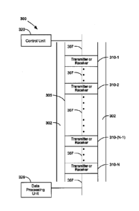
Figure 3 shows a block diagram of an embodiment of an example
system having a tool to make measurements to provide higher order azimuthal
sensitivity, in accordance with various embodiments. Tool 305 can have an
arrangement of transmitting sensors and receiving sensors such as transmitters
and receivers 310-1, 310-2 . . . 310-(N-1), 310-N structured relative to a
longitudinal axis 307 of tool 305. The transmitters and receivers 310-1, 310-2
. .
. 310-(N-1), 310-N can be arranged to provide multi-pole antenna operation. An
arrangement of transmitter antennas and receiver antennas can be structured
along longitudinal axis 307 of tool 305, which is substantially perpendicular
to
the cross section of the tool, for example corresponding to the cross section
of a
collar in a drill string.
The arrangement of transmitters and receivers 310-1, 310-2. . . 310-(N-
6
CA 02895018 2015-06-12
WO 2014/105084
PCT/US2012/072316
1), 310-N can be operated by selecting transmitter - receiver pairs defined by
the
spacing between the transmitter and the receiver in each respective pair.
Large
spacings can be used to probe ahead of the drill bit and acquire deep signals.
Smaller spacings can be used to probe in the formation regions around tool
305.
For example, a shallow measurement may include contributions from regions
about one inch to about 10 ft from the tool and a deep measurement may include
contributions from regions about 5 ft to about 200 ft from the tool.
Apparatus 300 can include a control unit 320 to control activation of the
transmitters of tool 305 and reception of signals at the receivers of tool
305.
Control unit 320 can be structured to be operable to select antennas of a
plurality
of antennas in one or more transmitter ¨ receiver pairs arranged to provide
higher order azimuthal sensitivity when the apparatus is operated downhole in
a
well. Control unit 320 can be operated in conjunction with data processing
unit
326 to process signals received from the receivers in tool 305.
Data processing unit 326 can be structured to be operable to process data
from one or more deep measurements. Data processing unit 326 can include
instrumentalities to perform one or more techniques to process signals from
the
receivers in the arrangement of transmitters and receivers 310-1, 310-2 . . .
310-
(N-1), 310-N. Data processing unit 326 also can use the generated signals to
determine formation properties around the borehole in which the tool is
disposed. Received signals at the tool may be used to make geosteering
decisions. Geosteering is an intentional control to adjust drilling direction.
The techniques to analyze the received signals can include various
applications of inversion operations, forward modeling, using synthetic logs,
and
filtering techniques. Inversion operations can include a comparison of
measurements to predictions of a model such that a value or spatial variation
of a
physical property can be determined. An inversion operation can include
determining a variation of electrical conductivity in a formation from
measurements of induced electric and magnetic fields. Other techniques, such
as
a forward model, deal with calculating expected observed values with respect
to
an assumed model. A synthetic log is a modeled log based on modeled response
of the tool in known formation parameters. The synthetic log is created by
numerically modeling the interaction of the tool and the formation, usually
7
CA 02895018 2015-06-12
WO 2014/105084
PCT/US2012/072316
involving simulation of each depth of the log point by point.
Control unit 320 and/or data processing unit 326 can be integrated with
tool 305 such that control unit 320 and/or data processing unit 326 are
operable
downhole in well 302. Control unit 320 and/or data processing unit 326 can be
distributed along tool 305. Control unit 320 and/or data processing unit 326
can
be located at the surface of well 302 operably in communication with tool 305
via a communication mechanism. Such a communication mechanism can be
realized as a communication vehicle that is standard for well operations.
Control
unit 320 and/or data processing unit 326 can be distributed along the
mechanism
by which tool 305 is placed downhole in well 302. Apparatus 300 can be
structured for an implementation in the borehole of a well as a measurements-
while-drilling (MWD) system such as a logging-while-drilling (LWD) system.
Alternatively, apparatus 300 may be configured in a wireline arrangement.
Figure 4A shows an embodiment of an example tool 405 operable as a
sensing system in an induction system to provide polarization focusing. The
tool
405 can be used in a system identical to or similar to system 300 of Figure 3.
The tool can be controlled in the induction system to provide a mechanism to
achieve a multi-pole sensing system. The tool 405 can be comprised of
transmitting sensor arrays and receiving sensor arrays in multiple stations.
Each
station may be composed of a multitude of sensors that are in different
orientations or that are operated with different signal amplitudes. The
transmitter stations and the receiver stations can be operated in a paired
arrangement. Each transmitting and receiving station pair, effectively, can
produce a single or a combination of higher order azimuthal modes in
sensitivity.
Examples of some modes are shown in Figure 2.
Multiple stations can be used to achieve different depth of detection and
can enhance sensitivity in the radial direction. Sensors at each station may
be
uniformly or non-uniformly disposed around a circumference of the tool
structure on which the sensors are disposed. The sensors may also form
arbitrary two-dimensional (2D) or 3D arrays. Even though achieving higher
azimuthal modes in sensitivity may rely on a specific relationship between
transmitting and receiving sensor positions, orientations, and strengths,
there can
be an infinite number of such arrangements. Each sensor can be realized as a
8
CA 02895018 2015-06-12
WO 2014/105084
PCT/US2012/072316
magnetic dipole, an electric dipole, or an electrode.
In order to excite higher-order azimuthal modes, orientations of the
dipoles in each substation can be varied, where an example is shown in Figures
4B-4C. In an embodiment, all sensors may be fed with a single wire and
alternating the winding direction of the wire as shown in the sensor feed
illustrated in Figure 4B. This allows a natural balance between different
sensors
strengths, since substantially the same current can pass through each sensor.
Separate wires can also be used for each sensor, as shown in the sensor feed
illustrated in Figure 4C. This can allow explicit control of the sensor
strengths
and help compensate for manufacturing differences between sensors.
Magnetic dipoles can be realized using either coils or solenoids.
Realizations of electric dipoles can include wire antennas, toroids, or
electrodes.
Due to the linearity of electromagnetic wave phenomenon in earth formations,
dipoles in different orientations can be synthetically combined after a
measurement to produce signals from hypothetical dipoles in different
orientations. A configuration that uses this is the tilted coil configuration.
Moreover, due to reciprocity, the roles of transmitter and receivers can be
interchanged without any change in the properties of the physics of the
application being addressed. A depth shift can be applied to signals from
transmitter-receiver station pairs that are not collocated and that have
substantially the same transmitter-receiver separation. The depth shift can be
adjusted to ensure different pairs are sensitive to substantially the same
volume
of formation.
Sensitivity of a sensor system that is composed of a transmitter and a
receiver is a product of the spatial transmission pattern of the transmitter
and
spatial reception pattern of the receiver. As a result, in order to have
azimuthal
sensitivity in the system, at least one of the transmitter or receiver has an
azimuthal transmission/reception pattern. It can be observed that having
azimuthal transmission/reception pattern for the sensors (for example via
multi-
pole antennas) does not directly lead to having a corresponding azimuthal
sensitivity for the combined transmitter-receiver system. In fact, specific
relationships between transmitter and receiver sensor positions and
orientations
are used to achieve deep high-order azimuthal sensitivity.
9
CA 02895018 2015-06-12
WO 2014/105084
PCT/1JS2012/072316
Figures 5A-5C show three example sensor configurations that can
achieve rith order azimuthal sensitivity. Each arrangement is comprised of n
transmitting dipole sensors. Figure 5A and Figure 5B show two sensor
arrangements comprised of n receiving dipole sensors in an addition to ii
transmitting dipole sensors. The third sensor arrangement, shown in Figure 5C,
is comprised of only one receiving sensor in an addition to n transmitting
dipole
sensors. The single receiving sensor of the third sensor arrangement is
disposed
along the axis of the tool. In Figures 5A-5C, riT, or, uir, oiR, and te
denote
radial position of the ith transmitter, angular position of the th transmitter
in
degrees, orientation vector of the ith transmitter, radial position of the ith
receiver,
angular position of the ith receiver in degrees and orientation vector of the
receiver. An orientation vector is a vector in the direction of the dipole of
the
sensor. The vectors ,3, qi and is are the unit vectors in cylindrical
coordinates
along radial, azimuthal, and z-directions. Since the orientation vector
relates to
direction only, an orientation vector ui is a unit vector The parameter a
is the
radius of the circle where the sensors are disposed, that is, it is the radius
of a
tool structure on which the sensor is disposed with the tool structure having
a
cylindrical shape. All of the dipoles in these arrangements can be of equal
strength. Figures 5A-5C provide only examples and different arrangements can
be achieved with the same effect by making modifications on sensor setup.
These modifications can include changing the position, orientation, strength
of
the dipoles, or combinations thereof.
Figures 6-8 show the sensor positioning and sensitivity for different
modes for the three arrangements shown in Figures 5A-5C, respectively. Within
each figure, there are four subfigures showing different modes. Mode number is
indicated above the subfigures. On the left-hand side of subfigures, sensor
position and orientation are shown. "In" and "Out" denote sensors pointing
inside and outside the circumference of the tool structure on which the
sensors
are mounted, respectively. "C" and "CC" denote sensors pointing clockwise and
counter clock-wise around the circumference of the tool structure,
respectively.
For each mode, the sensitivity in two dimensions is plotted next to its sensor
positions and orientations and the sensitivity in one dimension (1D) is
plotted to
CA 02895018 2015-06-12
WO 2014/105084
PCT/US2012/072316
the right of the 2D patterns. The data generating the 2D subplots can be
categorized or assigned to colors so that a display of the data generating the
2D
subplots indicates the magnitude of sensitivity by color, for example using
red
for positive and blue for negative.
Curves 672-1, 672-2, 674-1, 674-2, 676-1, 676-2, 678-1, and 678-2, in
the 1D subplots of Figure 6 indicate the geometric factor. Curves 672-3, 672-
4,
674-3, 674-4, 676-3, 676-4, 678-3, and 678-4 in the 1D subplots of Figure 6
indicate the integrated geometric factor. Curves 772-1, 772-2, 774-1, 774-2,
776-1, 776-2, 778-1, and 778-2, in the 1D subplots of Figure 7 indicate the
geometric factor. Curves 772-3, 772-4, 774-3, 774-4, 776-3, 776-4, 778-3, and
778-4 in the 1D subplots of Figure 7 indicate the integrated geometric factor.
Curves 871-1, 871-2, 872-1, 872-2, 873-1, 873-2, 874-1, and 874-2, in the 1D
subplots of Figure 8 indicate the geometric factor. Curves 871-3, 871-4, 872-
3,
872-4, 873-3, 873-4, 874-3, and 874-4 in the 1D subplots of Figure 8 indicate
the
integrated geometric factor. In the simulations for tools of operating
according
to the configurations in these figures, one transmitter station and one
receiver
station are separated axially by 10 ft with sensor radius a=4 inches with a
frequency 25 KHz used. Reference phase of all arrangements and modes was
chosen as 00, therefore maximum positive sensitivity is observed in all cases
at
0 . It is possible to rotate both the transmitters and the receivers to
achieve a
different phase in excitations. In general, two different phases for the same
mode are used to recover phase and amplitude information for a single mode.
Azimuthal sensitivity in all of the arrangements of Figures 5A-5C is
clearly seen in the top-most 2D subplots of Figures 6-8, while the bottom-most
1D subplots of Figures 6-8 show a sinusoidal pattern. The radial sensitivity,
as
shown in the top-most 1D subplot of Figures 6-8, indicates how deep the system
is sensing. It is observed that the first two arrangements (Figures 5A and 5B)
can produce deep sensing, while for the third arrangement (Figure 5C) sensing
depth decreases with increasing azimuthal modes. The middle 1D subplots of
Figures 6-8 shows the axial (z-) sensitivity, which corresponds to the
vertical
resolution of the tool. It is usually desirable to have a small width in axial
sensitivity plot for increased vertical resolution. However, narrow large
peaks
on wide plateaus of the middle 1D subplot indicate the so-called horn effect,
11
CA 02895018 2015-06-12
WO 2014/105084
PCT/US2012/072316
which is generally undesirable. It can be seen from the figures that the first
two
arrangements (Figures 5A and 5B) show some acceptable horn effect. The last
arrangement (Figure 5C) does not show any horn effect and it has larger
vertical
resolution.
In general, operation of the tool makes use of a combination of multiple
(N) high order azimuthal modes {ni, n2,...nN}. See, for example, Figure 2,
which indicates how to achieve azimuthal resolution by combining modes. In an
example embodiment, a superposition of arrangements in Figures 5A-5C with
different n can be used as the sensor arrangement. Moreover, two or more (N9)
different azimuthal phases for the same mode can be used to diversify
information. By azimuthal phase, it is meant that the same mode measurement is
taken but with the tool, both transmitter and receiver, rotated. This rotation
may
be applied by physically rotating the tool, or by providing a separate set of
sensors for the second phase. Providing a separate set of sensors for the
second
phase may almost double the total number of sensors. Multiple phases can be
especially useful in azimuthal focusing of the signal. The total number of
sensors in this case will be a sum of the number of sensors for all n = {ni,
n2,...nN} times N, minus the sensors that can be shared between different
modes
and phases.
Multi-pole excitation may achieved by introducing azimuthal variation
on a single sensor. An example of such variation includes varying the density
of
windings azimuthally on a toroid. In that case, a single sensor may be
adequate
to create higher order azimuthal modes. In addition, multi-pole excitation may
be achieved by subtracting the signal from a secondary station at a different
axial
position as bucking for reducing unwanted mode contributions such as the
direct
signal between transmitter and receiver. The concept of bucking is well known
and will not be discussed here.
A second pre-processing approach for a system can include taking the
ratio of signals from two different stations that obtain information from the
same
mode. By taking the ratio, effect of electronics drift or tool body
interference
may be eliminated. An approach that takes a ratio to eliminate such effects
has
been used for logging-while-drilling (LWD) propagation induction tools and can
be applied to embodiments of a system of multi-poles in an induction system to
12
CA 02895018 2015-06-12
WO 2014/105084
PCT/US2012/072316
provide polarization focusing. The use of a bucking approach and a ratio
approach may also double the number of sensors used in the system.
The arrangements shown in Figures 5A and 5B can produce azimuthal
sensitivity only for even numbers of azimuthal modes n, while the arrangement
of Figure 5C can produce azimuthal sensitivity for both even and odd numbers
of n. Being able to only use even numbers of modes translates to a 1800
azimuthal ambiguity in the spatial domain. The two arrangements shown in
Figures 5A and 5B allow deep sensing but have 1800 degree ambiguity. The
third arrangement, shown in Figure 5C, does not allow deep sensing; however,
it
does not suffer any ambiguity. A combination of these types of arrangements
can allow both deep sensing and partial or full resolution of azimuthal
ambiguity
in the sensing system.
Figure 9A illustrates an embodiment of an example a multi-pole
induction tool 905 via individually controlled coils. The tool 905 can be used
in
a system identical to or similar to system 300 of Figure 3. Figure 9B shows a
top down view of the individual coils around the circumference of the multi-
pole
induction tool of Figure 9A. The polarity of these coils can be electrically
controlled. Figure 9C shows, in table form, an embodiment of example
excitation polarities used for different modes to apply to the coils of the
multi-
pole induction tool 905. The label M refers to mode and the label P refers to
phase. The labels M and P are used in various of the figures associated with a
transmitting sensor (Trx) and a receiving sensor (Rev). As mentioned above, P
can be limited to phase 1 or phase 2 to remove azimuthal ambiguity in the
spatial
domain of the measurements. Though Figures 9B and 9C show 24 sensors in the
tool, the tool may have more or less than 24 sensors.
All sensors of the tool can be activated at the same time and with the
same frequency. However, they can also be activated at different times and
with
different frequencies, then synthetically summed in a processing unit. In one
approach, all modes (the whole table) can be excited at the same time with the
same frequency, and with the scaling K given in equation (2). This can
physically produce a directionally sensitive system. In a second approach, all
modes (the whole table) can be excited at the same time with different
frequencies with arbitrary scaling. In processing, all modes with multipliers
13
CA 02895018 2015-06-12
WO 2014/105084
PCT/US2012/072316
provided by K given in equation (2) can be summed. This approach
synthetically produces a directionally sensitive system. In a third approach,
each
mode (two rows of the table) can be excited at different times with arbitrary
frequencies and with arbitrary scaling. In processing, all modes with
multipliers
provided by K given in equation (2) can be summed. This approach
synthetically produces a directionally sensitive system.
Figure 10A illustrates an embodiment of an example a multi-pole
induction tool via rotating coils. The tool 1005 can be used in a system
identical
to or similar to system 300 of Figure 3. Figure 10B shows a top down view of
the individual coil as it is rotated around the circumference of the multi-
pole
induction tool 1005 of Figure 10A. The polarity of this coil can be
electrically
controlled. The polarity of the coil can be selected according to its position
as it
rotates around an axis of the tool 1005. Though Figure 10B only shows one coil
being rotated, both the transmitter coil and the receiver coil can be rotated.
The
coils can be rotated at the same rotation rate. Alternatively, the transmitter
coil
can be rotated with a first rotation speed and the receiver coil can be
rotated with
a second rotation speed, where the first rotation speed is different from the
second rotation speed. With the transmitter and receiver rotated, the tool
sonde
can be held stationary.
Figure 10C shows, in table form, an embodiment of example excitation
polarities used for different modes to apply to the coils of the multi-pole
induction tool at different angular positions around the circumference of the
tool
structure on which the coil is mounted. The label M refers to mode and the
label
P refers to phase. The labels M and P are used with each transmitting sensor
(Trx) and each receiving sensor (Rev). As mentioned above, P can be limited to
phase 1 or phase 2 to remove azimuthal ambiguity in the spatial domain of the
measurements. Though Figures 10B and 10C show 24 angular positions in the
tool, the coil of the tool may be rotated to more or less than 24 angular
positions.
In the multi-pole induction tool via rotating coils, the tool may be
operated using only a single transmitter sensor and single receiver sensor.
This
embodiment can be realized by having only one transmitter and one receiver in
one or more stations. Alternatively, the single transmitter and single
receiver
architecture can be realized with a number of transmitter sensors and a number
14
CA 02895018 2015-06-12
WO 2014/105084
PCT/US2012/072316
of receiver sensors in which only one transmitter sensor is activated to
transmit
and only one receiver sensor is activated to acquire a signal in response to
the
transmission. A measurement can be made the following manner. The upper
antenna housing is rotated to a first direction i. The lower antenna housing
can
be rotated to a second direction j. Measurement Kj can be obtained with the
two
antenna sensors at these positions. This two rotation and measure process can
be
repeated for all i=1.. .N, j=1.. .N. To obtain a result for a particular mode,
a
summation can be performed according to the operation
E(Mti x x Sri),
where Sti is the sign (+1 or -1) of the transmitter associated with the mode,
Srj is
the sign (+1 or -1) of the receiver associated with the mode. A hybrid of a
multi-
pole induction tool via individually controlled coils and multi-pole induction
tool
via rotating coils can be implemented by placing multiple antennas in the
upper
housing and multiple antennas in the lower housing and operating the hybrid
using excitations similar to those in Figures 9C and 10C.
Figure 11A illustrates an embodiment of an example a multi-pole
induction tool 1105 via periodic wrapping. The tool 1105 can be used in a
system identical to or similar to system 300 of Figure 3. The wrappings around
the tool can be arranged as periodic structures on the surface of the tool
structure
on which the wrapping sensors are mounted. The periodic wrapping can include
a transmitter wire and a receiver wire operatively controlled as a pair. Each
periodic wrapping disposed around the tool structure can include a first
portion
and a second portion, where the second portion can be directed azimuthally
back
towards the first portion such that in operation current flows in a same
azimuthal
direction in the first portion and in the second portion. The current flow is
shown by the arrows in Figure 11A.
The view in Figure 11A shows a cylindrical tool surface after cutting it
axially and opening it up. In operation, the right side of tool 1105 is
connected
to the left side of tool 1105. The periodicity can be provided as a wrapping
path
extending above, below, or above and below a plane perpendicular to the
longitudinal axis of the tool structure of tool 1105. As the wrapping is
disposed
azimuthally around tool 1105, its position in the z-direction along the axis
of tool
1105 varies periodically. The periodic variation is subject to manufacturing
CA 02895018 2015-06-12
WO 2014/105084
PCT/US2012/072316
tolerances. The tool 1105 is not limited to a cylindrical tool structure.
Though
sinusoidal shapes are shown in Figure 11A, shapes other than sinusoidal can be
used, such as triangular, rectangular, or other periodic structure.
Figure 11B shows an example periodic wrapping coupled to an excitation
source V, which can be used on the tool of Figure 11A. The periodic wrapping
can include first portion 1110-1 and a second portion 1110-2, where the second
portion 1110-2 can be directed azimuthally back towards the first portion 1110-
1
such that in operation current flows in a same azimuthal direction in the
first
portion 1110-1 and in the second portion 1110-2. As with Figure 11A, the view
in Figure 11B is provided with the tool surface after cutting it axially and
opening it up. With the wrappings disposed on operable tool 1105, the right
end
shown in Figure 11B almost touches left end shown in Figure 11B. With the
right end moved to almost touch the left end, it can be seen that the current
flows
in the same azimuthal direction, as the current arrows align. The example
wrapping of Figure 11B can be realized as a single continuous wire. The second
portion 1110-2 can be shifted 1800 from the first portion 1110-1 with respect
to
the tool structure. Alternatively, each winding can be composed of multiple
wires. Multiple wire segments can be concatenated to provide effectively a
single continuous wire.
A multi-pole induction tool 1105 via periodic wrapping can be structured
in a system with a control unit operatively coupled to the transmitter wire
and to
the receiver wire to selectively activate transmission from the transmitter
wire
and to selectively activate acquisition of a signal at the receiver wire in
response
to the transmission. The multi-pole induction tool via periodic wrapping can
include two periodic wrappings on the tool structure 1105, each of the two
periodic wrappings having a period different from each other. In another
embodiment, the multi-pole induction tool via periodic wrapping can include a
plurality of transmitter wires and a plurality of receiver wires operatively
controlled as pairs, with each transmitter wire and each receiver wire
disposed as
a periodic wrapping around the tool structure. Each periodic wrapping can
include a first portion and a second portion, with the second portion directed
azimuthally back towards the first portion such that in operation current
flows in
a same azimuthal direction in the first portion and in the second portion. In
the
16
CA 02895018 2015-06-12
WO 2014/105084
PCT/US2012/072316
plurality of transmitter wires and the plurality of receiver wires, each
transmitter
periodic wrapping can have a period equal to a period of a receiver periodic
wrapping to which it is operatively paired, where at least one pair having a
period different from another pair in the plurality.
The control unit can be structured to be operable to selectively activate a
transmitter wire and a receiver wire having the same periodicity of wrapping.
The control unit can be structured to be operable to control the plurality of
transmitter wires and the plurality of receiver wires as a plurality of
transmitter ¨
receiver pairs, the transmitter and the receiver of each transmitter ¨receiver
pair
having the same periodicity of wrapping. The transmitter wires and the
receiver
wires can be selectively controlled on a pair-wise basis.
The transmitter wires of a multi-pole induction tool can be disposed
along a longitudinal axis of the tool structure in a sequential manner with
respect
to the periodicity of each transmitter. In addition, the receiver wires can be
disposed along the longitudinal axis of the tool structure in a sequential
manner
with respect to the periodicity of each receiver. The sequential manner for
both
the transmitter wires and the receiver wires can be arranged from a largest
period
to a smallest period ordered by period size.
Figure 11C shows an example periodic wrapping, which can be used on
the tool of Figure 11A. Figure 11C shows a construction with the first portion
1110-3 and the second portion1110-4 structured as separate wires. The first
portion 1110-3 can have two ends to couple to a first source and the second
portion 1110-4 can have two ends to couple to a second source. The second
portion 1110-4 can be 180 shifted from the first portion 1110-3 with respect
to
the tool structure.
Figure 11D shows another example periodic wrapping, which can be
used on the tool of Figure 11A. Figure 11C shows a construction in which a
periodic wrapping can include wiring 1110-5 and 1110-6 internal to the tool
structure 1105.
The number of transmitting sensors and the number of receiving sensors
structured as periodic wrappings, as shown in Figure 11A, can be arranged to
generate deep high-order azimuthal sensitivity. However, the structure of
wrapping can be used in applications different from generating deep high-order
17
CA 02895018 2015-06-12
WO 2014/105084
PCT/US2012/072316
azimuthal sensitivity. The periodic wrapping structure can be used in
geosteering, mapping formation profile around a borehole, conducting a stress
analysis around the borehole, or other dovvnhole functions.
Figure 12 illustrates an embodiment of an example a multi-pole induction
tool 1205 via guided flux. The tool 1205 can be used in a system identical to
or
similar to system 300 of Figure 3. Coils with a high permeability core can be
used to achieve high mode numbers and balancing. Depending on the dipole
direction or position for a mode N that is of interested in, a high
permeability
core can be placed that opens outside at particular locations.
Figure 13 shows a block diagram of an embodiment of a system 1300,
such as a data acquisition system, having a tool operable as a sensing system
to
provide polarization focusing with transmitting antennas 1310-T-1 . . . 1310-T-
N and receiving antennas 1310-R-1 . . . 1310-R-M, operable in a borehole in
which the tool is placed. System 1300 can include a system control center
1320,
transmitters 1312-1 . . . 1312-N, receivers 1314-1 . . . 1314-M, a data
acquisition unit 1322, a data buffer 1324, a data processing unit 1326, and a
communication unit 1328 in addition to the tool with transmitting antennas
1310-T-1 . 1310-T-N and receiving antennas 1310-R-1 . . . 1310-R-M.
System control center 1320 can include a central processing unit (CPU), analog
electronics, digital electronics, or various combinations thereof to manage
operation of other units of system 1300.
System control center 1320 can generate a signal and feed the signal to
transmitters 1312-1 . . . 1312-N. The transmitters can be simultaneously or
sequentially activated and they can be kept on for a time long enough to allow
transients to die off and noise effects to diminish via stacking. The received
signals can be transformed into a domain where incident portion of the signal
can be separated from the reflected portion. The signals at the receivers arc
provided to system control center 1320, which can be stored at the data buffer
1324 before finally being communicated to the surface 1304.
System control center 1320 selectively activates the transmitting
antennas 1310-T-1 . . . 1310-T-N and selectively receives the signal scattered
from the formation at the receiving antennas 1310-R-1 . . . 1310-R-M. A mode
decoupler can be used to ensure mode purity by separating different modes from
18
CA 02895018 2015-06-12
WO 2014/105084
PCT/US2012/072316
mix modes. A mode adder can be used to produce a combination of modes that
has directional azimuthal sensitivity, such as shown in Figure 2. Due to
reciprocity, both a transmitter mode decoupler/adder 1327-T can be applied to
the transmitted signal and a receiver mode decoupler/adder 1327-R can be
applied to the received signal. A signal with a certain transient or periodic
signature is generated by the transmitting source. The receiver system
operation
may or may not be synchronized with the source activation. Synchronization
may allow better control on the phase of the received signal if no ratios are
being
used in processing. A received transient signal can be digitized and recorded
as
a function of time, and it can be later converted to frequency with a Fourier
transform operation. It can be alternatively passed through an analog band-
passed filter so that only the response at a discrete set of frequencies is
recorded.
The signal received by the receivers can be stored in the data buffer 1324,
processed, and if necessary, communicated to the surface.
Electromagnetic wave signals that are received at receiving antennas
1310-R-1 . . . 1310-R-M can be directed to corresponding receivers 1314-1 .
1314-M and system control center 1320. Operation of apparatus 1300 can
include multiple frequencies being transmitted and received at the same time
for
better time utilization. In such an operation, a sinusoidal waveform, a square
waveform, or other time-based waveforms may be used to excite multiple
frequencies simultaneously at each transmitting antenna 1310-T-1 . . . 1310-T-
N
or individual frequencies at transmitter antennas 1310-T-1 . . 1310-T-M.
Received signals corresponding to the multiple frequencies can be separated by
filters at the receiving end in data acquisition unit 1322. For each
transmitting
antenna 1310-T-1 . . . 1310-T-N, received signals at all receivers 1314-1 . .
.
1314-M can be recorded. Data buffer 1324 can be used to store received signal
for processing.
Data processing unit 1326 can be used to perform inversion or-other
processing on the data. The processing and the inversion can be continued in
accordance with processing features similar to or identical to embodiments
taught herein. Inversion operations can include a comparison of measurements
to predictions of a model such that a value or spatial variation of a physical
property can be determined. A conventional inversion operation can include
19
CA 02895018 2015-06-12
WO 2014/105084
PCT/US2012/072316
determining a variation of electrical conductivity in a formation from
measurements of induced electric and magnetic fields. Other techniques, such
as
a forward model, deal with calculating expected observed values with respect
to
an assumed model. In various embodiments, an inversion process, conducted
with respect to apparatus 1300, may be performed downhole or in an analysis
unit, such as a computer, at surface 1304 after the data is transferred to
surface
1304. Communication unit 1328 can communicate the data or results to surface
1304 for observation and/or determination of subsequent action to be taken in
a
drilling operation related to the measurements taken with apparatus 1300. The
data or results may also be communicated to other tools downhole and used to
improve various aspects of locating and extracting hydrocarbons.
Figure 14 shows an embodiment of an example processing methodology.
The signal obtained at the receivers are decoupled into different azimuthal
modes and also calibrated to remove effects of electronics drift or
amplification,
at 1410. The signal is then azimuthally focused by utilizing a combination of
azimuthal mode signals, at 1420. For some arrangements, such as configuration
1 of Figure 5A and configuration 2 of Figure 5B in Figures 6 and 7,
respectively,
since azimuthal sensitivity is the same at different radial distances from the
tool,
it can be successfully decoupled from the radial and axial dependence. The
next
step is radial focusing, and at this step, 1430, radial characteristics of the
target
are inverted by utilizing multiple station information. At the axial focusing
stage, at 1440, axial variation in the formation is recovered.
Radial and axial focusing can be similar to the well known software
focusing that is commonly used in standard array induction tools. Software
focusing works best in a tool operating regime where skin depth can be ignored
or successfully eliminated. A software focusing method can include generating
probe signals and making measuring at selected locations and using linearity
of
the measuring environment to determine quantities being measured from known
relationships between the generated entity (for example, a current or voltage
to
excite a transmitter) and measured property (voltage at a receiver) in the
measuring environment. In cases where this is not satisfied, a brute force
inversion, at 1450, can be used by utilizing a library, at 1470, or iterations
with a
forward method, at 1460. Inversion can include pattern matching, iterative
CA 02895018 2015-06-12
WO 2014/105084
PCT/US2012/072316
methods, or other inversion techniques. Inversion methods for induction tools
are well known and are not discussed further herein. The order of focusing and
inversion operations in Figure 14 can be interchanged based on the used
methodology.
The outputs of the focusing and inversion algorithm can be different in
different type of applications of embodiments of a multi-pole tool. In the
most
general case, a 3D profile of resistivity R(r, (1), z), dielectric
permittivity s(r, 4), z),
and dielectric permeability kr, 4), z) can be obtained, as shown at 1481. In
anisotropic formations, 3D horizontal and vertical properties of the formation
such as anisotropic resistivity Rh(r, 4), z), Rv(r, 4), z), anisotropic
dielectric
permittivity ch(r, 4), z), sv(r, 4), z), anisotropic dielectric permeability
i.th(r, 4), z),
mv(r, 4), z), and anisotropic dip and strike 0(r, 4), z), 4)(r, 4), z) can be
separately
obtained, at 1482. This general 3D profiling may use a large number of
stations
to achieve the desired radial resolution.
A less demanding parameterization of the problem assumes that the
formation is composed of non-circular concentric layers where formation
properties are the same within each layer. In this case, properties of each
layer
and the distance to each layer as a function of azimuthal angle can be
obtained as
distance to layer d(ib, 4), z), layer resistivity R(ib), layer dielectric
s(ib), layer
permeability gib), at 1483. An alternative is to assume that the layers are
stacked instead of being concentric to obtain boundary position x, y, z:
fcn(ib, x,
y, z) = 0, layer resistivity R(ib), layer dielectric s(ib), and layer
permeability gib),
at 1484.
A tool embodiment can also be used to image near well-bore features,
such as the distance of the borehole wall and invasion as distance to borehole
wall rb(4), z), borehole, invasion, formation resistivity Rb, R1, Rf,
borehole,
invasion, formation permittivity 61,, Ci, &f, borehole, invasion, formation
permeability [Lb, tf, at 1485. In this case, distance between the
transmitter
and receiver may be chosen in the order of borehole diameter for optimization.
In an LWD geosteering application, distance to a single layer can be mapped.
In
this case, the tool can be inside a reservoir, the shape of the boundary of
the cap
rock as a 3D image can be constructed and it can help keeping the tool within
the
21
CA 02895018 2015-06-12
WO 2014/105084
PCT/US2012/072316
most productive zone to provide distance to cap rock d(4), z), cap rock
resistivity
Rc(r, 4), z), and reservoir resistivity Rr(r, 4>, z), at 1486. In a geology
with a salt
dome, it may be possible to map the shape of the surface of the salt dome
using
distance to salt dome boundary d(I), z), at 1487. In this case, the
transmitting
and receiving station may be placed at different wellbores.
Figure 15 shows an embodiment of an example processing methodology.
The following methodology may work best in cases where skin effect is low,
which occurs when operating at lower frequencies, such as those in wireline
tools. At 1510, a received signal is subjected to decoupling and calibration.
The
decoupling and calibration can be conducted by applying, at 1512, a mode
decoupling and calibration matrix to raw data, as represented by
V f ,c)=
n-1
to provide decoupled and calibrated signal data, at 1522. At 1520, azimuthal
focusing can be applied to the decoupled/calibrated data. The azimuthal
focusing can be realized by applying a synthetic beam sweep, at 1524, to the
decoupled and calibrated signal data. The results of the synthetic beam sweep
can be subjected to deconvolution, at 1526. At 1530, inversion can be
performed to provide distance mapping, where the inversion can be conducted
using inputs of known layer resistivities, at 1532.
Due to design or imperfection of the transmitting system, a particular
excitation may produce a combination of different azimuthal modes. A
straightforward decoupling methodology can include characterizing mode
interference in an air hang test, where only direct signal from the same mode
is
supposed to be observed. In this case, all transmitting modes are activated,
and
all modes are received. This activity provides a coupling matrix V for
combinations of transmitting and receiving modes. The coupling matrix can be
inverted and stored for later use in decoupling of the signals. An alternative
that
can also achieve calibration is to place the tool in different test media that
are
known to excite only particular modes, at 1514. One particular choice of such
media is with resistivity R(r,(1),z) = Rocos(#nf/180). This media ideally
produces non-zero signal for the mode nf, and produces zero for all other
modes.
22
CA 02895018 2015-06-12
WO 2014/105084
PCT/US2012/072316
At 1516, measurement at mode n can be made and a voltage response matrix,
V(n, nf), can be constructed as a function of mode and azimuthal periodicity.
At
1518, a mode decoupling and calibration matrix can be calculated. This
calculated matrix can be generated as the inverse of the constructed voltage
response matrix.
Figure 16 shows mode mixing due to mechanical imperfection using
simulated results with such reference formation for different test formation
mode
nf. Azimuthal positions of the sensors are disturbed from their original
positions
randomly with 0.10, 1 , and 50 standard deviation. The upper figure shows ten
realizations of the sensor positions with the randomness as described above.
The
bottom figures show the amplitudes of the modes in the signal. The mode of the
reference formation is shown in between the double lines. In the ideal case
with
perfect positioning and balancing between the sensors, only the mode in
between
the lines should exist and all other modes should be zero. However, as it can
be
seen from the bottom figures, small deviations in the tool manufacturing can
also
excite other modes as well. For example, in the case of reference formation
mode 10, and a random deviation of 10, mode 10 is excited with an amplitude
range of 10-3 to 10-2. However, all modes from 1 up to 7 are excited with
normalized amplitudes from 10-2 to 1. This means that the tool is producing a
1000 times larger unwanted signal, along with the desired 10th mode signal. By
calculating a coupling matrix V(n,nf) and inverting it, it is possible to
decouple
individual modes. This operation not only decouples modes, but also calibrates
the signal strength and phase. It is possible to use other reference
formation,
such as a formation that is alternating between two values R(r,0,z) =
RoSign(onnfil 80). This test formation distribution may be easier to
manufacture
and use in calibration of tool hardware. Calculation of decoupling and
calibration matrix mentioned above can be applied before a logging job at the
surface. It can also be applied downhole by embedding and moving a material
that produces a reference signal within the tool body.
Since, each azimuthal mode provides one frequency in the azimuthal
domain, it is possible to combine different modes to obtain a focused
sensitivity
pattern. The formulas below can be used for this purpose
23
CA 02895018 2015-06-12
WO 2014/105084
PCT/US2012/072316
N _________________________________________ 41,0,0)\
V ift. = = A ) =ELK. = = Re e 18
= f
n=1 (1)
(1)
=2
P(i = 1) =IC
2
P(i = 2) = 0 (2)
nrxig(if, iõn,i R ref ,rf,0,z1, if n is even;
0, otherwise.
Here, V is the signal after azimuthal focusing, ib if and is are indices of
logging
depth, frequency, and spacing, (1)b is the focusing azimuth, N is the maximum
azimuthal mode, -1\19 is the number of different phases used in the tool
arrangement for the same mode, P is the phase used with index i,, g is the
Greens function that includes the tool and the reference formation as
described
in the decoupling stage above. The Greens function and associated coefficient
K
is only used for normalization purposes. Two phases N9=2 are enough to
recover both amplitude and phase information associated with each mode.
Figure 17 shows the azimuthal focusing results for different focusing
azimuths (1)b. Curves 1771, 1772, 1773, 1774, 1775, 1776, 1777, and 1778, in
the
1D subplots of Figure 17 indicate the geometric factor. Curves 1781, 1782,
1783, 1784, 1785, 1786, 1787, and 1788 in the ID subplots of Figure 17
indicate
the integrated geometric factor. It can be seen from the 2D figures and the ID
bottom-most figure that azimuthal focusing is successfully achieved.
By using different focusing azimuths, it is possible to scan the volume
around the tool. A drawback to the processing above may include ripples that
plague the azimuthal behavior. One way to remove the ripples is to utilize a
deconvolution filter. This filter can be constructed by first considering the
response of the tool in the case of a small step shaped (in azimuth) formation
R(rimpuise,0) with the definitions as below.
24
CA 02895018 2015-06-12
WO 2014/105084
PCT/US2012/072316
0 Or 1
r(1), - < ¨
N 180 N
. i ¨1 07r i
d(r,0)= < r(i), ¨ <--- < ¨ (3)
N 180 N
r(N), ifN ¨1 07C N
< <¨
, N 180 N
{Rf, if r<d(r,0)
(4)
RIõ otherwise.
1
0
(5)
rimpthe =
0
_ _
Here, d(r, A is the distance function as a function of a vector r and a scalar
azimuth 0. If the response of the tool to the impulse medium given above is
Vimp(ii,if,is,0b), the operations for deconvolution are shown in Figure 18. At
1810, the formation is simulated with an impulse resistivity. At 1820, voltage
associated with the impulse resistivity is calculated. At 1830, the calculated
voltage is deconvolved with measurement voltage data.
For a single station transmitter/receiver tool, if a step formation profile
with known resistivities and unknown distance is assumed, a table can be
constructed to convert from voltage level at each focusing azimuth to a
distance.
Construction of the table can be performed by utilizing the Greens function in
equation (2). With more information, more parameters can be obtained by
inversion. If multiple transmitter or receiver stations are available, more
parameters can be obtained and a 3D true formation resistivity map can be
constructed.
Figure 19 shows applications for an embodiment of a tool as discussed
herein. Such a tool can provide near-borehole properties of the formation and
assist in correction of other electromagnetic tool data (at 1920). Inversion
results
can also be used in geophysical/geomechanical interpretation (at 1930),
especially for deep reading, where spacing between transmitter and receiver is
large (10 ft to 100 ft). With the tool output (at 1910), it is possible to
construct
CA 02895018 2015-06-12
WO 2014/105084
PCT/1JS2012/072316
true 3D images of the formation providing visualization (at 1940) and use it
in
general formation evaluation purposes (at 1950). In various embodiments, a
multi-pole tool can also map layer boundaries around a reservoir and help
optimize geosteering (at 1960).
In various embodiments, a tool based on multi-poles, as discussed herein,
can achieve a large number of azimuthal modes. The tool can be implemented in
subterranean applications to achieve deep azimuthal focusing of sensitivity.
Deep 3D imaging of formations with azimuthal resolution higher than 20 may
be obtained. The tool may significantly improve geological evaluation of
formations and geosteering by accurately mapping layer boundary shapes. The
tool may also map borehole and invasion profile much deeper than it can be
achieved with the caliper or imaging tools.
Figures 20A-20D show four different simulated cases on the deep
imaging capability of an embodiment of a multi-pole tool. For the simulation
the background resistivity is taken to be 10 Om and shown in the 2D plots as
blank. The resistivity of the formation being imaged is 1 The processing
methodology discussed with respect to Figure 15 is used with 2, 4, 6, 8 and
10th
azimuthal modes and two phases as in equation (2). One transmitter station and
one receiver station separated by 20 ft with a sensor radius a=4 in and a
frequency of 25KHz is used in the simulations. The resistivity profile is
chosen
z-independent in simulations. Curves 2061, 2063, 2065, and 2067 show the
actual profile boundary, while curves 2062, 2064, 2066, and 2068 show the
inverted image of the profile boundary. It can be seen from Figures 20A-20D
that an embodiment of a multi-pole tool, as discussed herein, can successfully
construct an image of the formations around the tool.
In various embodiments, a system can comprise: a number of
transmitting sensors arranged on a tool structure; a number of receiving
sensors
arranged on the tool structure, the receiving sensor operable to acquire a
signal
in response to selective activation of the number of transmitting sensors,
such
that the number of transmitting sensors, the number of receiving sensors, or
both
the number of transmitting sensors and the number of receiving sensors include
one or more sensors structured as a multi-pole sensor, and the number of
transmitting sensors and the number of receiving sensors can be arranged to
26
CA 02895018 2015-06-12
WO 2014/105084
PCT/US2012/072316
generate deep high-order azimuthal sensitivity; and a control unit arranged to
control the selective activation of the number of transmitting sensors and to
acquire signals selectively from the number of receiving sensors in response
to
the selective activation.
The number of transmitting sensors can include one or more multi-pole
transmitter sensors and the number of receiving sensors can include one or
more
multi-pole receiver sensors, the one or more multi-pole transmitter sensors
and
the one or more multi-pole receiver sensors arranged to generate deep high-
order
azimuthal sensitivity. In addition, the number of transmitting sensors and the
number of receiving sensors can be arranged to establish deep high-order
azimuthal sensitivity by using a combination of magnetic dipoles. The number
of transmitting sensors and the number of receiving sensors can be arranged to
establish deep azimuthal focusing by using a combination of deep high-order
azimuthal sensitivity modes.
The number of transmitting sensors and the number of receiving sensors
can have an arrangement of n transmitting dipole sensors and n receiving
dipole
sensors such that placement of the n transmitting dipole sensors and the n
receiving dipole sensors with respect to the tool structure, in terms of /3,
and
unit vectors in cylindrical coordinates along radial, azimuthal and z-
directions
with the z-direction being along an axis of the tool structure, is given by
r1T=a
0,T = (4i _ 3)90
fif = _(_0,
= a
30
=¨(¨l),
with riT, 0,R, and id! denoting radial position of the ith
transmitter,
angular position of the ith transmitter in degrees, orientation vector of the
ith
27
CA 02895018 2015-06-12
WO 2014/105084
PCT/US2012/072316
transmitter, radial position of the ith receiver, angular position of the ith
receiver
in degrees, and orientation vector of the ith receiver, respectively, with a
being
the distance from the axis at which the transmitting dipole sensors and the
receiving dipole sensors are disposed.
The number of transmitting sensors and the number of receiving sensors
can have an arrangement of n transmitting dipole sensors and n receiving
dipole
sensors such that placement of the n transmitting dipole sensors and the n
receiving dipole sensors with respect to the tool structure, in terms of ,3, 0
and
unit vectors in cylindrical coordinates along radial, azimuthal and z-
directions
with the z-direction being along an axis of the tool structure, is given by
/IT = a
= (4i ¨ 5)L
z2T= (_1)i
15R = a
= (4i ¨5)90
=¨(-1)'
with rir, OT,uiT,e,e, and uf denoting radial position of the ith transmitter,
angular position of the ith transmitter in degrees, orientation vector of the
ith
transmitter, radial position of the ith receiver, angular position of the ith
receiver
in degrees, and orientation vector of the ith receiver, respectively, with a
being
the distance from the axis at which the transmitting dipole sensors and the
receiving dipole sensors are disposed.
The number of transmitting sensors and the number of receiving sensors
can have an arrangement of n transmitting dipole sensors and only one
receiving
sensor such that placement of the 11 transmitting dipole sensors and the only
one
receiving sensor with respect to the tool structure, in terms of ô, and unit
vectors in cylindrical coordinates along radial, azimuthal and z-directions
with
the z- direction being along an axis of the tool structure, is given by
28
CA 02895018 2015-06-12
WO 2014/105084
PCT/US2012/072316
T = a
= (4i ¨4)L0
uf =_f_Di
riR = 0
with Ty', oR, and le denoting radial position of the ith
transmitter,
angular position of the ith transmitter in degrees, orientation vector of the
ith
transmitter, radial position of the ith receiver, angular position of the ith
receiver
in degrees, and orientation vector of the ith receiver, respectively, with a
being
the distance from the axis at which the transmitting dipole sensors are
disposed.
In another example system, the number of transmitting sensors and the
number of receiving sensors arranged to generate deep high-order azimuthal
sensitivity can include a transmitter wire and a receiver wire operatively
controlled as a pair, each of the transmitter wire and the receiver wire
disposed
as a periodic wrapping around the tool structure, each periodic wrapping
including a first portion and a second portion, the second portion directed
azimuthally back towards the first portion such that in operation current
flows in
a same azimuthal direction in the first portion and in the second portion. The
periodic wrapping can be arranged as a single wire having two ends to couple
to
a source, the second portion being 180 shifted from the first portion with
respect to the tool structure. The single wire can include wire segments that
are
concatenated. The first portion and the second portion can be separate wires,
the
first portion having two ends to couple to a first source and the second
portion
having two ends to couple to a second source, the second portion being 180
shifted from the first portion with respect to the tool structure. Each
periodic
wrapping can include wiring internal to the tool structure. The periodic
wrapping, including internal wiring, can be arranged as a single wire having
two
ends.
The example system can include two periodic wrappings on the tool
structure, each of the two periodic wrappings having a period different from
each
other. The example system can include a plurality of transmitter wires and a
plurality of receiver wires operatively controlled as pairs, each transmitter
wire
and each receiver wire disposed as a periodic wrapping around the tool
structure,
29
CA 02895018 2015-06-12
WO 2014/105084
PCT/1JS2012/072316
each periodic wrapping including a first portion and a second portion, the
second
portion directed azimuthally back towards the first portion such that in
operation
current flows in a same azimuthal direction in the first portion and in the
second
portion, each transmitter periodic wrapping having a period equal to a period
of
a receiver periodic wrapping to which it is operatively paired, at least one
pair
having a period different from another pair. The transmitter wires can be
disposed along a longitudinal axis of the tool structure in a sequential
manner
with respect to the period of each transmitter, and the receiver wires can be
disposed along the longitudinal axis of the tool structure in a sequential
manner
with respect to the period of each receiver. The sequential manner for both
the
transmitter wires and the receiver wires can be from a largest period to a
smallest
period ordered by period size. The periodic wrapping of the transmitter wire
can
be sinusoidal, triangular, or rectangular.
The example system can include a data processing unit operable with the
control unit such that from generation of a number of deep high-order
azimuthal
sensitivity modes, the data processing unit can be structured to synthetically
sum
the deep high-order azimuthal sensitivity modes to establish deep azimuthal
focusing. The example system can include a mode adder operable with the
control unit such that from generation of a number of deep high-order
azimuthal
sensitivity modes, the mode adder can be structured to sum the deep high-order
azimuthal sensitivity modes to establish deep azimuthal focusing.
In a second example system, the number of transmitting sensors and the
number of receiving sensors arranged to generate deep high-order azimuthal
sensitivity can include multiple dipole antennas having controlled polarity,
the
control unit arranged to selectively control the polarity of the multiple
dipole
antennas. The transmitting sensors of the multiple dipole antennas can be
arranged in a transmitter station with each transmitting sensor at a different
angular position around a circumference of the tool structure, the transmitter
station disposed in an array of transmitter stations. A multiple dipole
antenna
operable as one of the receiving sensors can be arranged as a receiver station
in
an array of receiver stations. In an embodiment, the receiver station can have
multiple dipole antennas operable as receiving sensors with each receiving
sensor of the receiver station at a different angular position around a
CA 02895018 2015-06-12
WO 2014/105084
PCT/US2012/072316
circumference of the tool structure with respect to the other receiving
sensors in
the station. The transmitter stations and the receiver stations can be
disposed
along a longitudinal axis of the tool separate to operatively provide a range
of
depths of investigation.
The number of transmitting sensors can be magnetic dipoles selected
from a group including coils and solenoids or the number of transmitting
sensors
can be electric dipoles selected from a group including wire antennas,
toroids,
and electrodes. The transmitting sensors can include a toroid having windings
such that a density of the windings is varied azimuthally on the toroid.
The second example system can include a data processing unit operable
with the control unit such that from generation of a number of deep high-order
azimuthal sensitivity modes, the data processing unit can be structured to
synthetically sum the deep high-order azimuthal sensitivity modes to establish
deep azimuthal focusing. The second example system can include a mode adder
operable with the control unit such that from generation of a number of deep
high-order azimuthal sensitivity modes, the mode adder can be structured to
sum
the deep high-order azimuthal sensitivity modes to establish deep azimuthal
focusing.
In a third example system, the number of transmitting sensors and the
number of receiving sensors arranged to generate deep high-order azimuthal
sensitivity can include multiple dipole antennas operable under controlled
rotation by the control unit. One or more of the multiple dipole antennas can
be
operable as transmitting sensors disposed in a housing different from one or
more of the multiple dipole antennas operable as the receiving sensors. The
control unit can be operable to rotate one or more of the multiple dipole
antennas
operable as transmitting sensors at a rotation speed different from a rotation
speed of one or more of the multiple dipole antennas operable as receiving
sensor. In an embodiment, only one of the multiple dipole antennas is operated
as a rotating transmitter sensor. The third example system can include a data
processing unit operable with the control unit such that from generation of a
number of deep high-order azimuthal sensitivity modes, the data processing
unit
can be structured to synthetically sum the deep high-order azimuthal
sensitivity
modes to establish deep azimuthal focusing. The third example system can
31
CA 02895018 2015-06-12
WO 2014/105084
PCT/US2012/072316
include a mode adder operable with the control unit such that from generation
of
a number of deep high-order azimuthal sensitivity modes, the mode adder can be
structured to sum the deep high-order azimuthal sensitivity modes to establish
deep azimuthal focusing.
Various embodiments of a system can include a data processing unit
operable to: decouple acquired signals into different azimuthal modes and
calibrate the one or more signals, generating decoupled and calibrated signal
data; perform azimuthal focusing, radial focusing, axial focusing, and
inversion
based on the dccoupled and calibrated signal data; and generate data related
to
one or more of the borehole and the formation.
In various embodiments, a method can comprise: activating one or more
transmitting sensors of a tool disposed in a borehole to transmit into a
formation;
selectively acquiring one or more signals at one or more receiving sensors of
the
tool in response to transmission by the one or more transmitting sensors,
wherein
the one or more transmitting sensors, the one or more receiving sensors, or
both
the one or more transmitting sensors and the one or more receiving sensors
include one or more sensors structured as a multi-pole sensor; and controlling
the activation and the selective acquisition, generating deep high-order
azimuthal
sensitivity. The one or more transmitting sensors can include one or more
multi-
pole transmitter sensors and the one or more receiving sensors can include one
or
more multi-pole receiver sensors, the one or more multi-pole transmitter
sensors
and the one or more multi-pole receiver sensors arranged to generate the deep
high-order azimuthal sensitivity. Generating deep high-order azimuthal
sensitivity can include establishing the deep high-order azimuthal sensitivity
by
using a combination of magnetic dipoles. Generating deep high-order azimuthal
sensitivity includes establishing the deep high-order azimuthal sensitivity by
using a combination of deep high-order azimuthal sensitivity modes.
The one or more transmitting sensors and the one or more receiving
sensors can have an arrangement of n transmitting dipole sensors and n
receiving
dipole sensors such that placement of the n transmitting dipole sensors and
the n
receiving dipole sensors with respect to the tool structure, in terms of ô,
q'$ and
is unit vectors in cylindrical coordinates along radial, azimuthal and z-
directions
with the z-direction being along an axis of the tool structure, is given by
32
CA 02895018 2015-06-12
WO 2014/105084
PCT/US2012/072316
= a
= (4i _ 3)90_
fir =¨(¨l)3
R = a
= (4i _ 5)90
with riT, or, oR, and uiR denoting radial position of the ilk
transmitter,
angular position of the ith transmitter in degrees, orientation vector of the
ith
transmitter, radial position of the ith receiver, angular position of the ith
receiver
in degrees, and orientation vector of the ith receiver, respectively, with a
being
the distance from the axis at which the transmitting dipole sensors and the
receiving dipole sensors are disposed.
The one or more transmitting sensors and the one or more receiving
sensors can have an arrangement of n transmitting dipole sensors and n
receiving
dipole sensors such that placement of the n transmitting dipole sensors and
the n
receiving dipole sensors with respect to the tool structure, in terms of j3 ,
0 and
unit vectors in cylindrical coordinates along radial, azimuthal and z-
directions
with the z-direction being along an axis of the tool structure, is given by
r,T = a
= (4i _ 5) 9 __0__
air =
r,R = a
R = (4i ¨5)90¨n
(47 =¨(-1)'ô
with riT,or5uir,riR, õ, and u/ denoting denoting radial position of the ith
transmitter,
angular position of the ill' transmitter in degrees, orientation vector of the
ith
transmitter, radial position of the ith receiver, angular position of the ith
receiver
in degrees, and orientation vector of the ith receiver, respectively, with a
being
33
CA 02895018 2015-06-12
WO 2014/105084
PCT/US2012/072316
the distance from the axis at which the transmitting dipole sensors and the
receiving dipole sensors are disposed.
The one or more transmitting sensors and the one or more receiving
sensors can have an arrangement of n transmitting dipole sensors and only one
receiving sensor such that placement of the n transmitting dipole sensors and
the
only one receiving sensor with respect to the tool structure, in terms of 3,
and i unit vectors in cylindrical coordinates along radial, azimuthal and z-
directions with the z-direction being along an axis of the tool structure, is
given
by
= a
= (4i ¨ 4)0
= 0 i
ri = 0
ui = z
with riT, or, riR R
and uf denoting radial position of the ith transmitter,
angular position of the ith transmitter in degrees, orientation vector of the
ith
transmitter, radial position of the ith receiver, angular position of the ith
receiver
in degrees, and orientation vector of the jthreceiver, respectively, with a
being
the distance from the axis at which the transmitting dipole sensors are
disposed.
In another example method, the one or more transmitting sensors and the
one or more receiving sensors arranged to generate the deep high-order
azimuthal sensitivity can include a transmitter wire and a receiver wire
operatively controlled as a pair, each of the transmitter wire and the
receiver
wire disposed as a periodic wrapping around the tool structure, each periodic
wrapping including a first portion and a second portion, the second portion
directed azimuthally back towards the first portion such that in operation
current
flows in a same azimuthal direction in the first portion and in the second
portion.
The periodic wrapping can be arranged as a single wire having two ends to
couple to a source, the second portion being 180 shifted from the first
portion
with respect to the tool structure. The first portion and the second portion
can be
separate wires, the first portion having two ends to couple to a first source
and
34
CA 02895018 2015-06-12
WO 2014/105084
PCT/1JS2012/072316
the second portion having two ends to couple to a second source, the second
portion being 1800 shifted from the first portion with respect to the tool
structure. In an embodiment, each periodic wrapping can include wiring
internal
to the tool structure.
In an embodiment, the one or more transmitting sensors and the one or
more receiving sensors can include two periodic wrappings on the tool
structure,
each of the two periodic wrappings having a period different from each other.
In
another embodiment, the one or more transmitting sensors and the one or more
receiving sensors can include a plurality of transmitter wires and a plurality
of
receiver wires operatively controlled as pairs, each transmitter wire and each
receiver wire disposed as a periodic wrapping around the tool structure, each
periodic wrapping including a first portion and a second portion, the second
portion directed azimuthally back towards the first portion such that in
operation
current flows in a same azimuthal direction in the first portion and in the
second
portion, each transmitter periodic wrapping having a period equal to a period
of
a receiver periodic wrapping to which it is operatively paired, at least one
pair
having a period different from another pair.
The example method can include generating a number of deep high-order
azimuthal sensitivity modes and synthetically summing the deep high-order
azimuthal sensitivity modes to establish deep azimuthal focusing. The example
method can include generating a number of deep high-order azimuthal
sensitivity modes and summing, using a mode adder, the deep high-order
azimuthal sensitivity modes to establish deep azimuthal focusing.
In a second example method, generating deep high-order azimuthal
sensitivity can include selectively controlling polarity of multiple dipole
antennas. The second example method can include generating a number of deep
high-order azimuthal sensitivity modes and synthetically summing the deep
high-order azimuthal sensitivity modes to establish deep azimuthal focusing.
The second example method can include generating a number of deep high-order
azimuthal sensitivity modes and summing, using a mode adder, the deep high-
order azimuthal sensitivity modes to establish deep azimuthal focusing.
In a third example method, generating deep high-order azimuthal
sensitivity can include controllably rotating a number of multiple dipole
CA 02895018 2015-06-12
WO 2014/105084
PCT/US2012/072316
antennas. Controllably rotating multiple dipole antennas can include rotating
only one transmitter sensor. The third example method can include generating a
number of deep high-order azimuthal sensitivity modes and synthetically
summing the deep high-order azimuthal sensitivity modes to establish deep
azimuthal focusing. The third example method can include generating a number
of deep high-order azimuthal sensitivity modes and summing, using a mode
adder, the deep high-order azimuthal sensitivity modes to establish deep
azimuthal focusing.
Various embodiments of a method can include processing the one or
more signals, the processing can include: decoupling one or more signals into
different azimuthal modes and calibrating the one or more signals, generating
decoupled and calibrated signal data; performing azimuthal focusing, radial
focusing, axial focusing, and inversion based on the decoupled and calibrated
signal data; and generating data related to one or more of the borehole and
the
formation from performing the azimuthal focusing, the radial focusing, the
axial
focusing, and the inversion. Decoupling and calibrating the one or more
signals
can include: simulating the formation with an impulse resistivity; generating
a
simulated signal voltage from simulating the formation with the impulse
resistivity; and deconvolving a measured signal voltage with the simulated
signal
voltage.
Various embodiments of a method can include prior to deploying the tool
in the borehole, generating and storing, in memory, a mode decoupling and
calibration matrix such that the one or more signals can be decoupled and
calibrated in operation of the tool in the borehole using the mode decoupling
and
calibration matrix, the mode decoupling and calibration matrix generated by:
operating the tool in a known formation with azimuthal periodicity; making
measurements at a selected mode; constructing a response matrix based on the
measurements for the selected mode and azimuthal periodicity; and inverting
the
response matrix.
Different embodiments of systems and methods of operating system, as
taught herein, can be combined in a number of arrangements. The combination
can include permutations of features of the systems, permutations of features
of
methods of operating the systems, or permutations of features of the systems
and
36
CA 02895018 2015-06-12
WO 2014/105084
PCT/US2012/072316
features of methods of operating the systems.
In various embodiments, a machine-readable storage device can have
instructions stored thereon, which, when executed by one or more processors of
a machine, cause the machine to perform operations, the operations comprising
any of the features of methods of making measurements via multi-pole induction
and analyzing the measurements in a manner identical to or similar to the
methods described herein. Further, a machine-readable storage device, herein,
is
a physical device that stores data represented by physical structure within
the
device. Examples of machine-readable storage devices include, but are not
limited to, read only memory (ROM), random access memory (RAM), a
magnetic disk storage device, an optical storage device, a flash memory, and
other electronic, magnetic, and/or optical memory devices.
In various embodiments, a system can comprise a tool having an array of
transmitters and an array of receivers; a control unit operable to manage
generation of signals from the array of transmitters and to manage collection
of
received signals at the array of receivers; and a data processing unit,
wherein the
tool, the control unit, and the data processing unit are structured to operate
according to any of the features of methods of making measurements via multi-
pole induction and analyzing the measurements in a manner identical to or
similar to the methods described herein. The system can include one or more
machine-readable storage devices to implement one or more of these features.
Figure 21 depicts a block diagram of features of an embodiment of a
system 2100 including a sensor tool 2105 having an arrangement of transmitters
and receivers operable as a multi-pole induction tool. The arrangements of
transmitters 2110-1 and receivers 2110-2 of sensor tool 2105 can be realized
similar to or identical to arrangements discussed herein. The arrangements can
include one or more transmitter-receiver antenna pairs arranged to be
selectively
controlled to generate deep high-order azimuthal sensitivity. For example,
control of the one or more transmitter-receiver antenna pairs can include, but
is
not limited to, selective polarity of the transmitter and the receiver in the
transmitter-receiver antenna pairs.
System 2100 can also include a controller 2141, a memory 2142, an
electronic apparatus 2143, and a communications unit 2145. Controller 2141,
37
CA 02895018 2015-06-12
WO 2014/105084
PCT/US2012/072316
memory 2142, and communications unit 2145 can be arranged to operate sensor
tool 2105 as a multi-pole antennas to provide higher order azimuthal modes.
Controller 2141, memory 2142, and electronic apparatus 2143 can be realized to
control activation of transmitter antennas 2110-1 and selection of receiver
antennas 2110-2 in sensor tool 2105 and to manage processing schemes in
accordance with measurement procedures and signal processing as described
herein. Communications unit 2145 can include downhole communications in a
drilling operation. Such downhole communications can include a telemetry
system.
System 2100 can also include a bus 2147, where bus 2147 provides
electrical conductivity among the components of system 2100. Bus 2147 can
include an address bus, a data bus, and a control bus, each independently
configured. Bus 2147 can also use common conductive lines for providing one
or more of address, data, or control, the use of which can be regulated by
controller 2141. Bus 2147 can be configured such that the components of
system 2100 are distributed. Such distribution can be arranged between
downhole components such as transmitters 2110-1 and receivers 2110-2 of
sensor tool 2105 and components that can be disposed on the surface of a well.
Alternatively, the components can be co-located such as on one or more collars
of a drill string or on a wireline structure.
In various embodiments, peripheral devices 2146 can include displays,
additional storage memory, and/or other control devices that may operate in
conjunction with controller 2141 and/or memory 2142. In an embodiment,
controller 2141 can be realized as one or more processors. Peripheral devices
2146 can be arranged with a display with instructions stored in memory 2142 to
implement a user interface to manage the operation of sensor tool 2105 and/or
components distributed within system 2100. Such a user interface can be
operated in conjunction with communications unit 2145 and bus 2147. Various
components of system 2100 can be integrated with sensor tool 2105 such that
processing identical to or similar to the processing schemes discussed with
respect to various embodiments herein can be performed downhole in the
vicinity of the measurement or at the surface.
Figure 22 depicts an embodiment of a system 2200 at a drilling site,
38
CA 02895018 2015-06-12
WO 2014/105084
PCT/US2012/072316
where the system 2200 includes a tool 2205 configured with sensors operable as
a system of multi-pole antennas. A control unit and processing unit of the
tool
2205 can be distributed among system 2200 or can be integrated with tool 2205
providing for control and analysis activities to be conducted downhole. The
tool
2205 can be realized in a similar or identical manner to arrangements and
processing discussed herein to make measurements in a borehole and to process
the signals and data generated from signals acquired at the tool 2205.
The system 2200 can include a drilling rig 2202 located at a surface 2204
of a well 2206 and a string of drill pipes, that is, the drill string 2208,
connected
together so as to form a drilling string that is lowered through a rotary
table 2207
into a wellbore or borehole 2212. The drilling rig 2202 can provide support
for
the drill string 2208. The drill string 2208 can operate to penetrate the
rotary
table 2207 for drilling the borehole 2212 through subsurface formations 2214.
The drill string 2208 can include drill pipe 2218 and a bottom hole assembly
2220 located at the lower portion of the drill pipe 2218.
The bottom hole assembly 2220 can include a drill collar 2215, the tool
2205 attached to the drill collar 2215, and a drill bit 2226. The drill bit
2226 can
operate to create the borehole 2212 by penetrating the surface 2204 and the
subsurface formations 2214. The tool 2205 can be structured for an
implementation in the borehole 2212 as a MWD system such as a LWD system.
The housing containing the tool 2205 can include electronics to activate one
or
more transmitters of the tool 2205 and collect responses from one or more
receivers of the tool 2205. Such electronics can include a processing unit to
provide formation analysis, borehole analysis, or combinations thereof to the
surface over a standard communication mechanism for operating a well.
Alternatively, electronics can include a communications interface to provide
signals output by receivers of the tool 2205 to the surface over a standard
communication mechanism for operating a well, where these output signals can
be analyzed at a processing unit at the surface to provide formation analysis,
borehole analysis, or combinations thereof.
During drilling operations, the drill string 2208 can be rotated by the
rotary table 2207. In addition to, or alternatively, the bottom hole assembly
2220 can also be rotated by a motor (e.g., a mud motor) that is located
downhole.
39
CA 02895018 2015-06-12
WO 2014/105084
PCT/US2012/072316
The drill collars 2215 can be used to add weight to the drill bit 2226. The
drill
collars 2215 also can stiffen the bottom hole assembly 2220 to allow the
bottom
hole assembly 2220 to transfer the added weight to the drill bit 2226, and in
turn,
assist the drill bit 2226 in penetrating the surface 2204 and subsurface
formations 2214.
During drilling operations, a mud pump 2232 can pump drilling fluid
(sometimes known by those of skill in the art as "drilling mud") from a mud
pit
2234 through a hose 2236 into the drill pipe 2218 and down to the drill bit
2226.
Thc drilling fluid can flow out from the drill bit 2226 and be returned to the
surface 2204 through an annular area 2240 between the drill pipe 2218 and the
sides of the borehole 2212. The drilling fluid may then be returned to the mud
pit 2234, where such fluid is filtered. In some embodiments, the drilling
fluid
can be used to cool the drill bit 2226, as well as to provide lubrication for
the
drill bit 2226 during drilling operations. Additionally, the drilling fluid
may be
used to remove subsurface formation 2214 cuttings created by operating the
drill
bit 2226.
In various embodiments, the tool 2205 may be included in a tool body
2270 coupled to a logging cable 2274 such as, for example, for wireline
applications. The tool body 2270 containing the tool 2205 can include
electronics to activate one or more transmitters of the tool 2205 and collect
responses from one or more receivers of the tool 2205. Such electronics can
include a processing unit to provide formation analysis, borehole analysis, or
combinations thereof to the surface over a standard communication mechanism
for operating a well. Alternatively, electronics can include a communications
interface to provide signals output by receivers of the tool 2205 to the
surface
over a standard communication mechanism for operating a well, where these
output signals can be analyzed at a processing unit at the surface to provide
formation analysis, borehole analysis, or combinations thereof. The logging
cable 2274 may be realized as a wireline (multiple power and communication
lines), a mono-cable (a single conductor), and/or a slick-line (no conductors
for
power or communications), or other appropriate structure for use in the
borehole
2212.
Tools and methods that utilize multi-pole antennas identical to or similar
CA 02895018 2015-06-12
WO 2014/105084
PCT/1JS2012/072316
to embodiments discussed herein may used to produce deep azimuthal focusing
of electromagnetic waves and to construct deep 3D images of electromagnetic
properties of formations from a single well. This may allow new geological
profiling applications and also significantly improve evaluation of
formations.
Data from this tool may be used to optimize drilling and production
operations.
Although specific embodiments have been illustrated and described
herein, it will be appreciated by those of ordinary skill in the art that any
arrangement that is calculated to achieve the same purpose may be substituted
for the specific embodiments shown. Various embodiments use permutations
and/or combinations of embodiments described herein. It is to be understood
that the above description is intended to be illustrative, and not
restrictive, and
that the phraseology or terminology employed herein is for the purpose of
description. Combinations of the above embodiments and other embodiments
will be apparent to those of skill in the art upon studying the above
description.
41