Note: Descriptions are shown in the official language in which they were submitted.
CA 02904139 2015-09-03
WO 2014/159479 PCT/US2014/023855
DIRECT FLUID INDICATORS IN MULTIPLE SEGMENT PROSPECTS
Background
[0001] Seismic indicators or anomalies such as flat spots, conformance, and
amplitude versus
offset ("AVO") have been used in recent years to improve the estimation of the
chance of
success ("COS") of segments and prospects. A "segment" generally refers to a
discrete
exploration target, and a prospect refers to a collection of segments. The
"prospect chance of
success" generally is the chance that at least one segment succeeds (i.e., has
hydrocarbons)
assuming that each of the segments in the prospect is drilled.
[0002] Several methods exist to handle these anomalies. At least one approach
employs
Bayesian Risk Modification ("BRM"). This approach allows the exploration team
to take into
account anomalies that increase the chance of success of a segment, and "false
positive"
anomalies, i.e., anomalies that are caused by a particular fluid condition
inside the reservoir and
that may be mistaken for hydrocarbon indicators. For this reason, these
signals are generally
regarded as direct fluid indicators ("DFIs") and not as direct hydrocarbon
indicators ("DHIs").
[0003] A challenge when dealing with seismic anomalies is how the seismic
information in
multi-segment prospects should be valued.
Summary
[0004] Systems, methods, and computer-readable media are disclosed, which may
be
implemented for determining a chance of success for a prospect including a
plurality of
segments. For example, the method may include receiving seismic data
indicative of a plurality
of anomalies in a prospect. Prior probabilities of success and failure
scenarios may be computed
for at least one of the segments included in the prospect. Likelihoods of the
anomalies may be
determined given the success and failure scenarios for the at least one of the
segments included
in the prospect. The segments may be classified into different direct fluid
indicator dependency
groups. A degree of correlation may be determined between the anomalies for
the of the direct
fluid indicator dependency group. A posterior chance of success may be
determined for the
prospect based at least in part on the degree of correlation between the
anomalies.
1
81791276
[0004a] According to an aspect of the present disclosure, there is provided a
method for
determining a chance of success for a prospect in a subterranean formation,
comprising:
receiving seismic data that is produced in response to a seismic survey of the
prospect,
wherein the seismic data is indicative of a plurality of anomalies in the
prospect, wherein the
prospect includes a plurality of segments; computing prior probabilities of
success and failure
scenarios for at least one of the segments; determining likelihoods of the
anomalies given the
success and failure scenarios for the at least one of the segments;
classifying at least two of
the segments as part of a direct fluid indicator dependency group; determining
a degree of
correlation between the anomalies for the direct fluid indicator dependency
group;
determining a posterior chance of success for the prospect based at least in
part on the degree
of correlation between the anomalies; and updating a model of the subterranean
formation
based at least in part on the posterior chance of success for the prospect,
wherein the model is
configured to be used to determine a presence of hydrocarbons in one or more
of the segments
in the prospect in the subterranean formation.
10004b] According to another aspect of the present disclosure, there is
provided a computing
system, comprising: a display; a processor; and a memory system comprising one
or more
non-transitory computer readable media storing instructions thereon that, when
executed by
the processor, are configured to cause the computing system to perform
operations, the
operations comprising: receiving seismic data that is produced in response to
a seismic survey
of a prospect in a subterranean formation, wherein the seismic data is
indicative of a plurality
of anomalies in the prospect, and wherein the prospect includes a plurality of
segments;
computing prior probabilities of success and failure scenarios for at least
one of the segments;
determining likelihoods of the anomalies given the success and failure
scenarios for the at
least one of the segments; classifying at least two of the segments as part of
a direct fluid
indicator dependency group; determining a degree of correlation between the
plurality of
anomalies for the direct fluid indicator dependency group; determining a
posterior chance of
success for the prospect based at least in part on the degree of correlation
between the
anomalies; and updating a model of the subterranean formation based at least
in part on the
posterior chance of success for the prospect, wherein the model is configured
to be used to
determine a presence of hydrocarbons in one or more of the segments in the
prospect in the
subterranean formation.
2
Date Recue/Date Received 2020-09-08
81791276
[0004c] According to another aspect of the present disclosure, there is
provided a non-
transitory computer-readable medium storing instructions thereon that, when
executed by a
processor, are configured to cause the processor to perform operations, the
operations
comprising: receiving seismic data that is produced in response to a seismic
survey of a
prospect in a subterranean formation, wherein the seismic data is indicative
of a plurality of
anomalies in the prospect, and wherein the prospect includes a plurality of
segments;
computing prior probabilities of success and failure scenarios for at least
one of the segments;
determining likelihoods of the anomalies given the success and failure
scenarios for the at
least one of the segments; classifying at least two of the segments as part of
a direct fluid
indicator dependency group; determining a degree of correlation between the
anomalies for
the direct fluid indicator dependency group; determining a posterior chance of
success for the
prospect based at least in part on the degree of correlation between the
anomalies; and
updating a model of the subterranean formation based at least in part on the
posterior chance
of success for the prospect, wherein the model is configured to be used to
determine a
presence of hydrocarbons in one or more of the segments in the prospect in the
subterranean
formation.
2a
Date Recue/Date Received 2020-09-08
81791276
[0005] It will be appreciated that the foregoing summary is merely intended to
introduce a
subset of the subject matter discussed below and is, therefore, not limiting.
Brief Description of the Drawings
[0006] The accompanying drawings, which are incorporated in and constitute a
part of this
specification, illustrate embodiments of the present teachings and together
with the description,
serve to explain the principles of the present teachings. In the figures:
[0007] Figure 1 illustrates a hierarchical chain with four risk groups,
according to an
embodiment.
[0008] Figure 2 illustrates an initial risk assessment display, according to
an embodiment.
[0009] Figure 3 illustrates an initial fluids and reservoir probabilities
display, according to an
embodiment.
[0010] Figure 4 illustrates a DFI assessment display, according to an
embodiment.
[0011] Figures 5-1 illustrates a graph showing Optimal k vs. P(shared) for
COS(A) = 0.6 and
COS(B) = 0.3, according to an embodiment.
[0012] Figures 5-2 illustrates a graph showing Optimal k vs. P(shared) for
COS(A) = 0.6 and
COS(B) = 0.6, according to an embodiment.
[0013] Figure 6 illustrates a flowchart of a method for assessing a prospect
analysis in the
presence of multiple DFI anomalies, according to an embodiment.
[00141 Figure 7 illustrates a flowchart of a method for determining a
posterior prospect COS,
according to an embodiment. The term PFRM means Pore Fluid and Rock Matrix
Conditions,
and it refers to the possible failure conditions (scenarios).
10015] Figure 8 illustrates a schematic view of a computing system, according
to an
embodiment.
[0016] Figure 9 illustrates a view of two illustrative segments A and B whose
"Reservoir
Presence" probability is estimated to be respectively 0.3 and 0.2, according
to an embodiment.
2b
Date Recue/Date Received 2020-09-08
CA 02904139 2015-09-03
WO 2014/159479 PCT/US2014/023855
Detailed Description
[0017] The following detailed description refers to the accompanying drawings.
Wherever
convenient, the same reference numbers are used in the drawings and the
following description
to refer to the same or similar parts. While several embodiments and features
of the present
disclosure are described herein, modifications, adaptations, and other
implementations are
possible, without departing from the spirit and scope of the present
disclosure.
[0018] The methodology disclosed herein may be generic and valid for any kind
of anomaly,
whether seismic, EM (electromagnetic), or of other kind. In the following,
examples seismic
anomalies are considered, since this may be one example of use of the
technology; however,
there is neither reason nor intent to limit the scope of the disclosure to
such an implementation.
[0019] As part of a Bayesian Risk Modification ("BRM") approach, a range of
hypotheses
concerning segment or prospect conditions may be developed and may lead to
observed seismic
indicators and/or anomalies. These hypotheses are then quantified into
different "likelihood
values." A "likelihood value" generally refers to the probability that the
observed anomaly
exists given a success or a failure scenario. The terms "Scenario" and "Case"
may be used
herein in an interchangeable manner. The observed anomaly becomes a new piece
of
information that is used to update the prior estimate of chance of success
("COS") and volume
based on the original geological and geophysical considerations. Likelihood
values and prior
estimates are combined following a Bayesian framework that states that the
posterior COS is
proportional to the prior estimate multiplied by the likelihood calculated
from the data, e.g.:
P(OillAnomaly) = P(AnomalylOil)*P(Oil) / P(Anomaly).
[0020] Using a computer program such as, for example, GEOX software (developed
and
distributed by SCHLUMBERGER), the user may implement a segment analysis.
Considering a
single segment, the COS of geological elements in the segment may be assigned
certain risk
factors by geologists. The product of these risk factors may determine the COS
of the segment.
This quantity may be referred to as "prior COS," ignoring any anomalies. In
Table 1 below,
"reservoir presence," "reservoir quality," and "source and migration" are
confirmed, while there
may be an uncertainty about the presence or the effectiveness of the "trap and
seal". In this
example, the prior COS is equal to 0.1.
3
CA 02904139 2015-09-03
WO 2014/159479 PCT/US2014/023855
110,$k:::: factor P P (segment I
Trap and seal 1.0 0.1
Reservoir presence 1.0 1.0
Reservoir quality 1.0 1.0
Source and migration 1.0 1.0
[0021] When starting the direct fluid indicator ("DFI") assessment, the user
may define and
assess the possible background conditions that could give rise to a specific
anomaly. In an
example, a single failure scenario exists (e.g., brine), with a prior
probability equal to 1-COS.
The procedure may be extended to the case with multiple failure scenarios.
[0022] After the identification of these conditions, the user may input the
likelihood of the DFI
for each scenario, as shown in Table 2:
Table 2
Label
.. P (DPI I ease)
Oil & evaluated reservoir 0.8
Water & evaluated reservoir 0.3
[0023] In this example case, a greater likelihood of the observed DFI for the
success scenario
(e.g., oil & evaluated reservoir) is estimated than for the failure scenario
(e.g., water & evaluated
reservoir). The posterior COS may then be calculated using the Bayes formula,
as shown in
Table 3:
t!.
Label P (DFI I ease) P (case, success) P (case, failure)
P (case & P (case I DPI)
.. _ DFI) ...
Oil & eval. res 0.8 0.1 0.080 0.229
Water & eval. 0.3 0.9 0.270 0.771
res
[0024] This means that, in this example case, the anomaly boosts the initial
COS from 0.1 to
0.229.
[0025] The risk factors may be updated at the segment level. Embodiments of
the methods
disclosed herein may promote a fast and accurate update of the risk factors.
As the term is used
herein, "accurate" generally means the system may explicitly compute the
updated probabilities
of each risk factor given the seismic observation, e.g., without performing a
Monte Carlo
sampling. In order to obtain this result, a hierarchical chain may be
followed.
[0026] Figure 1 illustrates a hierarchical chain 100 with four risk groups
102, 104, 106, 108,
according to an embodiment. Each risk group 102, 104, 106, 108 may include one
or more risk
4
CA 02904139 2015-09-03
WO 2014/159479 PCT/US2014/023855
factors. The risk factors may have the same relevance for concurring to the
determination of the
COS. The hierarchy may be functional for the algorithm presented herein. The
probability of
each risk group 102, 104, 106, 108 may be updated using the DFI information
and the
information from the risk groups that are above, except, for example, risk
group 102, which has
no risk groups above it in this instance. Accordingly, the reservoir quality
may be updated,
given the DFI and the reservoir presence. Within each risk group 102, 104,
106, 108, the
proportions of the original assessment (pre-DFI) may be maintained.
[0027] Table 4 below may be illustrative, as it includes four examples of risk
factors:
Table 4
" Risk factor P ( P (segment
Trap and seal 1.0 0.3
Reservoir presence 1.0 0.5
Reservoir quality 1.0 0.8
Source and migration 1.0 0.6
[0028] In this example, the factors "trap and seal" and "source and migration"
belong to the
hydrocarbon presence group. These values may be reported in the initial risk
assessment tab of
the GeoX program, as shown in Figure 2, although any other suitable
application or platform
may be employed.
[0029] In an "initial fluids and reservoir probabilities display," which may
be provided as a tab
in a computer program, for example, as shown in Figure 3, the different
failure liquids and the
different non-reservoir lithologies may be received as inputs into the system.
In this example,
the failure condition is water, and the non-reservoir condition is shale
(labeled "Non reservoir
1").
[0030] Next, the system and/or method may assign the likelihoods to the
success and failure
scenarios. In Table 5, the success scenario is the scenario with greatest
likelihood, followed by a
success scenario with poor reservoir quality, a shale case, and a scenario
with the reservoir filled
with brine.
Table
Label P (11)F1 ease)
Oil & evaluated reservoir 0.8
Oil & non evaluated reservoir 0.6
Water & evaluated reservoir 0.3
Water & non evaluated reservoir 0.3
Shale 0.5
CA 02904139 2015-09-03
WO 2014/159479 PCT/US2014/023855
[0031] The "DFI assessment" display or tab may be used for assigning the
likelihood values, as
shown in Figure 4. In Figure 4, the word "Label" is used to distinguish a
particular scenario, and
therefore, it is used as a synonym for the word "Scenario" or "Case." As will
be seen, the COS
given DFI is updated in the right part of the table. In this case, the update
reflects a belief
(likelihood) and the prior information (original COS), following the Bayes
formula. The COS is
consequently boosted from 7.2% to 13.0%, because:
COS*P(DFI 'success) 0.072*0.8
COS DFI - ____________ 0.130
P(DFI) 0.441
[0032] Finally, in the "DFI modified risk" tab, the updated probabilities for
each risk factor may
be found. The first quantity, P(RP DFI), wherein "RP" refers to "reservoir
presence" 102
(Figure 1) may be calculated as follows:
P(RP DFI) =
= P (RP, Success DFI) E?,-1 P(RP, Failurei IDFI )
= P (RP Success, DFI) * P(SuccessIDFI) + 71_1P (RP IFaili, DPI) P(Fail ilDFI)
= 1* 0.130 * 1 + 1 * 0.024 + 1*0.223 + 1*0.056 + 0*0.566 = 0.434
[0033] The remaining quantities may be computed in a similar way, taking into
consideration the
hierarchical structure of the chain, as shown in Figure 1. Examples of the
remaining quantities
are shown in Table 6 below:
= RwIgOpy P (play) ...,,,,Agm, P (segment
Trap and seal 1.0 0.497
Reservoir presence 1.0 0.434
Reservoir quality 1.0 0.815
Source and migration 1.0 0.743
>Marginal play probability 1.0
>Conditional segment probability 0.130
>Unconditional probability 0.130
Dry hole risk 0.870
[0034] When two risk factors belong to the same risk group, their proportion
may be maintained
as in the original risk assessment. This is the case of the factors "trap &
seal" and "source &
migration." Originally, the log-proportion of "trap & seal" is:
log (Trap&Seal) log(0.3)
_________________________________________________________ = 0.702
log(Trap&Seal * Source&Migration) log(0.3 * 0.6)
The log-proportion of "source & migration" is: 1-0.702=0.298.
6
CA 02904139 2015-09-03
WO 2014/159479 PCT/US2014/023855
[0035] Given the DFI and the first two risk groups of the present example, a
joint updated
probability for "trap and seal" and "source and migration" is equal to 36.92%.
To compute the
marginal updated probability of "trap & seal," therefore:
P(TS DFI, RP, RQ) = 0.36920702 = 0.497, and
P(SM DFI, RP, RQ) = 0.3692'298 = 0.743,
where TS is "trap and seal," RP is "reservoir presence," RQ is "reservoir
quality" and SM is
"source and migration" as defined above.
[0036] In this situation, the probability of reservoir presence decreases from
0.5 to 0.43 due to
a relatively high likelihood of the shale scenario with respect to the other
failure scenarios. The
boost in the COS is, therefore, a result more of hydrocarbon presence elements
("source and
trap") than the reservoir presence, in this example, since a scenario with no
reservoir has a
relatively large likelihood.
[0037] The foregoing discloses an embodiment of a method for computing the
updated risk
factors estimates given a single DFI. The following discloses embodiments of a
method for
computing risk factor estimates in multiple segment prospects.
[0038] In this embodiment, the method may include determining the DFI in multi-
segment
prospects. Prospects that include multiple segments have a COS that is equal
to or greater than
the COS of the segment that has the highest COS. If the COS of the different
segments are
independent, then the COS of the prospect increases with the number of
segments in the
prospect. The prospect COS is the chance that at least one segment is
successful, assuming that
each of the segments is tested (e.g., drilled). Further, as described above,
anomaly information
such as a flat spot, conformance, etc. boosts the COS of a segment. Similarly,
lack of anomaly
information, when expected, attenuates the COS of the segment.
[0039] Turning now to how the anomalies' value may be estimated and assessed
in multi-
segment prospects, scenarios are considered in which the segments are
independent. Scenarios
are also considered where the segments are partially or completely risk
dependent. Further, it
will be seen that considering the anomalies as distinct pieces of information
in both types of
scenarios may be misleading.
[0040] Considering a prospect with two segments, located on either side of a
fault, an anomaly
may be recorded and interpreted for both segments. In seismic surveys, it may
be difficult to
determine whether the anomaly relates to the first or the second segment. In a
similar situation,
7
CA 02904139 2015-09-03
WO 2014/159479 PCT/US2014/023855
an implementation that considers the two anomalies as distinct pieces of
information may lead to
a large and unrealistic boost of the COS, since the presence of an anomaly
generally increases
the COS.
[0041] An embodiment of the present method, however, includes introducing DFI
dependency
groups, i.e., groups of segments that totally or partially share a DFI signal.
The user may classify
(e.g., enroll) segments as part of these groups and define the degree of
correlation that the user
believes is present in the anomalies. In other words, the user may introduce
an explicit link
between the DFI signals. This link may be controlled by a DFI correlation
parameter -k" whose
range of values is from 0 to 1.
[0042] A group with k=0 describes a situation where the anomalies recorded in
the segments in
the group are independent. A group with k=1 describes a situation where the
DFI may be
completely correlated (e.g., connected, linked, or associated), and,
therefore, there is no
additional information brought by the observation of several anomalies. A
group with 0 <k < 1
(e.g., k=0.5) means that there is a partial correlation between the DFI
signals.
[0043] It is possible to have situations where multiple segments are part of
the same prospect,
but the segments may be different from each other in terms of geological
structure or
geographical location. In those cases, situations may be modeled in which the
DFI may be
correlated just within a subgroup of segments.
[0044] The procedure presented here holds whether the segments are independent
or risk-
dependent. In this latter case, the risk elements associated with different
segments within a
prospect may be correlated through a shared geological control. The shared
geological control
may be used to model dependency among different segments. The presence and the
probability
of such control elements may be decided according to an understanding about
the geology of the
prospect. In general, a large probability of a geological control may
correspond to a large degree
of independence among the segments (since, as an example, the risk may lie on
the independent
branch of the tree), while a small probability corresponds to a highly risk-
dependent situation
(since in this example case, most of the risk lies in the shared geological
control itself).
[0045] Figure 9 illustrates an example situation with two segments A and B
whose "Reservoir
Presence" probability is estimated to be respectively 0.3 and 0.2. We know
that the two
segments A, B likely represent two distinct branches 902, 904 of the same
depositional system
900. However, complete dependency among the two branches 902, 904 may not be
assumed;
8
CA 02904139 2015-09-03
WO 2014/159479 PCT/US2014/023855
instead dependency up to a certain degree may be determined e.g., by the
position of the dot 906
in Figure 9. The dot 906 is in this example is the last point of common
deposition, following the
direction of the arrow 908, for the two segments A, B, and it may act as a
shared geological
control. In order to quantify the correlation, we may be able to assess the
probability of such
geological control, e.g., the probability that the deposition has reached the
dot 906. Given that
the deposition has reached the geological control, the branches 902, 904 may
be totally
independent, leading to the two segments A, B.
[0046] Embodiments of the present disclosure may provide an explicit way to
model the
correlation between seismic signals leading to the DFI. Using one or more
embodiments of the
present disclosure, this explicit connection may be introduced by assuming
that the higher this
correlation is in place within segments classified (e.g., enrolled) in the
same DFI dependency
group, the more the DFI signals will share the same kind of information. This
is made possible
through the definition of a "reference DFI" signal that will be described in
greater detail below.
[0047] Turning to modeling the process through the introduction of the DFI
correlation
parameter "k," when the DFI correlation parameter k=0, a model of a scenario
where the
probability of observing an anomaly in a certain segment is consistent with
the likelihood that
the user has assigned to a given segment may be desired. In this case, it is
assumed that the DFI
signals are independent within the dependency group.
[0048] Assuming an example simple segment with a single failure scenario
(water), and
likelihood values for oil and brine equal 0.8 and 0.3, respectively, the
following relationships are
produced in Table 7:
Table 7 '
Label (case) P (DFI I case)
Oil & evaluated reservoir 0.8
Water & evaluated reservoir 0.3
[0049] This is equivalent to Table 8 below, where it is explicitly recognized
that the
independence of the DFI signal under consideration from the DFI reference
segment, indicated
with DFI_ref. The third column of this table shows the probability of DFI for
this segment,
given the scenario and the presence or absence of the DFI in the reference
segment.
9
CA 02904139 2015-09-03
WO 2014/159479 PCT/US2014/023855
Table 8
Label (case) Label (DFI ref) P (DFI I case, DFI ref)
Oil & evaluated reservoir Present 0.8
Water & evaluated reservoir Present 0.3
Oil & evaluated reservoir Absent 0.8
Water & evaluated reservoir Absent 0.3
[0050] Likewise, when k=1 (maximum correlation among the seismic signals
within the DFI
dependency group), the presence or absence of the signal in a given segment
may be completely
correlated with the presence or absence of the DFI reference signal. This
dependency is reflected
in Table 9 below:
Table 9
?i Label (DFI ret) (DFI I DII ret)
Present 1
Absent 0
[0051] Also in this case, the complete table may be displayed, as shown in
Table 10 below:
,
Table 10
Label (case) Label (DFI ref) , P (DFI I case, DFI ref)
Oil & evaluated reservoir Present 1
Water & evaluated reservoir Present 1
Oil & evaluated reservoir Absent 0
Water & evaluated reservoir Absent 0
[0052] An example solution may include using the parameter k to build a linear
interpolation
between these two extreme scenarios. This linear interpolation may, however,
not translate into
a linear interpolation of the resulting COS, since the effect of this
probability distribution is
combined with a series of other probability distributions that define the
dependency among risk
factors.
[0053] The resulting Table 11 assigns the following weights to each scenario:
õ
Table 11
= Label (case) Label (DFI ref) P (DFI I
case, DFI ref)
Oil & evaluated reservoir Present 0.8+k*(1-0.8)
Water & evaluated reservoir Present 0.3+k*(1-0.3)
Oil & evaluated reservoir Absent 0.8-k*0.8
Water & evaluated reservoir Absent 0.3-k*0.3
[0054] Table 11 may be interpreted to mean that the higher the value of the
DFI correlation
parameter k, the more the DFI may resemble the reference DFI, ensuring the
required
correlation. Table 11 above, therefore, may represent the Conditional
Probability Table ("CPT")
that describes the probability distribution of the DFI signal, given the
segment's COS and the
CA 02904139 2015-09-03
WO 2014/159479 PCT/US2014/023855
DFI reference segment (DFI ref). The method may be extended in case of
multiple failure
scenarios. The choice of the DFI reference segment may be automatic. In other
words, the
segment may have sampled uniformly among each of the segments that belong to
the
dependency group.
[0055] In some cases, a change of paradigm in the modeling of the DFI
anomalies may be
implemented. For example, embodiments of the present disclosure may sample the
DFI signals
using the likelihoods provided, e.g., by the user, and the CPTs generated,
e.g., by the processor
executing the software, and then produce an estimate of the COS by analyzing
the number of
success cases versus the total number of samples. This approach is consistent
with a Monte
Carlo architecture of the entire risking scheme.
[0056] The DFI correlation parameter k may have a range of admissible values,
e.g., between 0
and 1, as noted above. The lower bound of this range is 0, i.e., the user may
assume that its DFI
signals are completely uncorrelated. The upper bound of the range may be
computed by
identifying the maximum correlation coefficient among the segments that
belongs to the defined
DFI dependency group. In some cases, this may not be calculated upper bound,
but an upper
bound dictated by a geological knowledge of the process.
[0057] For pairs of segments that belong to the considered DFI dependency
group, the "Pearson
correlation coefficient" may be determined. In the particular case of
distributions with binary
outcomes (oil/dry), the bivariate distribution of the COS for two segments X
and Y, may be
derived and this coefficient explicitly computed as shown in Table 12:
;pr 'Fable 12
!!i X / Y = d .!!!!! Y= oil .!!!!: marginal
X= dry N 00 N 0 1 N OX
X=oil N10 N11 N 1 X
Marginal N OY N 1 Y
[0058] In this table, NO0 represents the number of Monte Carlo trials where
both X and Y are
unsuccessful, N01 represents the number of trials where Y alone is successful,
N10 represents
the number of cases where X alone is successful, N11 represents the number of
cases where both
X and Y are successful, NOX represents the number of cases where X is dry and
N are the total
MC runs. The correlation coefficient p may be then computed as:
N11*N00¨N10*N01
pXY- , _______________________
v (NOX*N1X*NOY *NIT)
11
CA 02904139 2015-09-03
WO 2014/159479 PCT/US2014/023855
[0059] Once the Pearson coefficients are determined, the maximum of the range
may be set as a
maximum admissible value of the range and the average as suggested value for
the parameter
"k". Without external information, the DFI correlation may reflect the
geological risk
correlation present among the segments. The choice presented here is one
illustrate way to set
the DFI correlation parameter, and it is not to be intended as the sole
possible choice.
[0060] An insight into a relationship between risk dependency and the DFI
correlation
coefficient k may be seen using the two graphs shown in Figures 5-1 and 5-2.
As shown, pXY
vs. P(shared) is plotted for a prospect with two segments A and B, and a
single risk factor. There
is an inverse proportionality relationship between these two quantities.
Further, as shown in this
example, when the two COS are equal, the largest value for the DFI correlation
parameter "k" is
1, while when the two COS are different, the largest value for "k" is lower
than 1 because of the
asymmetric behavior of the prospect COS.
Examples
[0061] The present systems and methods may be further understood with
reference to the
following one or more non-limiting examples.
[0062] An illustrative example may be represented by an example prospect. This
example
prospect has a 4-way closure and a 3-way fault-dependent closure. The two
closures are
separated by a saddle at 1060 m. A spill point for the combined structure is
1080 m.
[0063] In this example, an anomaly may be observed both on the 4-way closure
and on the 3-
way closure. The 4-way closure has been assessed as two different segments,
because of a fault
that divides the structure. The 4-way closure has a high chance for a
successful trap (80%).
There is a slight chance that the seal could be breached by a thief zone or
sub-seismic faulting.
The 3-way closure is riskier and has a 30% chance for an adequate fault seal.
There is no trap
risk dependency between the two closures. The targets are in the same sand,
which has a 35%
chance of being present. The targets, therefore, share a reservoir risk
dependency. The targets
share the same chance of "source and migration." Estimates of the shared play
and conditional
segment probabilities for the two segments that compose the 4-way closure are
shown in Table
13 below:
12
CA 02904139 2015-09-03
WO 2014/159479 PCT/US2014/023855
Table 13
Risk factor P (play) P (segment I play) Overall risk
Trap & seal [%] 100 80 80
Reservoir Presence [%] 70 50 35
Reservoir Quality [%] 100 100 100
Source and Migration [%] 80 80 64
COS (Unconditional probability) 17.9
[0064] The equivalent estimates for the 3-way closure are shown in Table 14:
Table 14
Risk factor P (play) P (segment I play) , Overall risk
Trap & seal [%] 100 80 50
Reservoir Presence [%] 70 50 35
Reservoir Quality [%] 100 100 100
Source and Migration [%] 80 80 64
COS (Unconditional probability) 11.2
[0065] These example segments are in the same play and have the same shared
play risks.
They also have the same conditional reservoir presence and source and
migration risks. The sole
difference is the higher risk on "trap and seal" for the 3-way closure. As
shown, the initial COS
of the two segments composing the 4-way structure is 17.9%, while the initial
COS for the 3-way
is 11.2%.
[0066] Considering water as the failure fluid condition and shale as the non-
reservoir
condition, two possible failure scenarios and one possible success scenario
are present. The
probability of shale is 1-P(res)=0.65 for the three segments. The probability
of water and
reservoir is P(Water & Res) = (1-P(T&S)*P(S&M))*P(Res) and is respectively
equal to:
(1-0.8*0.64)*0.35 = 0.171 for the two segments composing the 4-way closure,
and
(1-0.5*0.64)*0.35 = 0.238 for the 3-way closure segment.
[0067] The likelihoods estimated by the geologists are consistent with the
observation: the
strongest anomaly is observed in correspondence of the 4-way closure, and a
weaker anomaly in
correspondence of the 3-way structure. The following likelihoods may thus be
assessed:
P(DFI I Oil & eval. res.) = 0.8 (0.6 for the 3-way)
P(DFI 1Water & eval. res.) = 0.3 (0.3 for the 3-way)
P(DFI 1Water & not. eval. res.) = 0.2 (0.4 for the 3-way)
13
CA 02904139 2015-09-03
WO 2014/159479 PCT/US2014/023855
As a result, an updated COS for the 4-way and for the 3-way closure may be
determined as
follows:
4way: P(Oil & eval. Res DFI) = P(DFI Oil & eval. res) * P(Oil & eval. res.) /
P(DFI)
= 0.8 * 0.179 / 0.325 = 0.442
3 way: P(Oil & eval. Res DFI) = P(DFI Oil & eval. res) * P(Oil & eval. res.) /
P(DFI)
= 0.6 * 0.112 / 0.399 = 0.169
[0068] The analyses of the three segments may be included as part of (e.g.,
enrolled in) the
prospect analysis of this example prospect. There is full risk dependency
among the three
segments in terms of "reservoir presence" as well as "source and migration."
The "trap and seal"
risk factor is assessed as partially dependent (P(shared)=0.9) for the two
segments belonging to
the 4-way structure.
[0069] The prior prospect COS is 20.87% (this comes from
0.64*0.35*1*(0.864+0.5-0.864*0.5),
where 0.864 is the probability that the 4-way trap works, and it is computed
as 0.9*(1-0.2*0.2)).
The prospect COS with DFI is 78.24% if we regard the DFI signals in the two
segments that
compose the 4-way structure as independent. This may not be a good
representation of the
scenario, and therefore these two segments may be classified as part of (e.g.,
enrolled in) a DFI
dependency group.
[0070] The first computation may be used to determine the correlation
coefficient between the 4-
way A and the 4-way B segments. For this case study the correlation matrix
(produced with a
Monte Carlo sampling of the COS of the two segments without DFI) may be seen
in Table 15
below:
Table 15
::
4-wayA / 4 wayB Success 1Failure 1 .. :]i]] .. Failure 2
.. Marginal
VIII M! (brine) O. A]
(shale) .!!"
Success 0.159 0.020 0 0.179
Failure 1 (brine) 0.020 0.151 0 0.171
Failure 2 (shale) 0 0 0.65 0.65
Marginal 0.179 0.171 0.65 1
[0071] The matrix is symmetrical in this particular case, since the two
segments are assessed in
an identical manner, in terms of risk dependency. Since the correlation of the
COS is at issue,
the failure scenarios may be grouped, allowing the following compact version
of the correlation
matrix to be derived as shown in Table 16:
14
CA 02904139 2015-09-03
WO 2014/159479 PCT/US2014/023855
Table 16.
1-a /4 %% Success Failure Mat ginal
Success 0.159 0.020 0.179
Failure 0.020 0.801 0.821
Marginal 0.179 0.821 1
[0072] Note that the marginals match the original COS shown previously. Now,
to compute the
correlation coefficient, the following may be used:
0.159*0.801-0.020*0.020 - 0.865
pXY-
v (0.179*0.821*0.179*0.821)
[0073] This is a coefficient that resumes the degree of correlation that
exists between the two
segments classified (e.g., enrolled) in the DFI dependency group. This will be
the maximum
value allowed for the correlation of the DFI signal. Since the segments have a
geological risk
correlation of 0.865, it might not be possible that the DFI have a higher
degree of correlation.
This might prevent the user from introducing artificially high correlations in
the anomalies that
do not reflect the geology of the prospect. Since in this DFI dependency group
there are just two
segments, this value is also the suggested value for the DFI dependency
factor.
[0074] With this value for the factor "k", the CPT may be modified as
prescribed. In Monte
Carlo samples, the reference node among 4-way A and 4-way B may be sampled,
and the
modified CPT used to introduce correlation in the DFI signals.
[0075] With this new analysis, the updated prospect COS becomes 53.72%. The
boost is
attenuated by the fact that an 86% correlation between the anomalies of the 4-
way closure is
introduced. Without this correlation in place, an updated COS of 78.24 % is
calculated, as
shown previously. This concludes the example. In the next three paragraphs we
will discuss
some implementation details related to this example.
[0076] Within the defined dependency group, made by segments 4-way A and 4-way
B, the
reference node may be sampled. In this case, the two segments are identical,
and so it does not
matter which of the two is chosen. Assuming that 4-way A is chosen as the
reference, the DFI
likelihoods of the segment 4-way A follow the CPT shown in Table 17:
Tabk 17
fiiiiiiIIMEMEMENEMEMIMEENA
Oil & eval. Res. 0.8
Brine & eval. Res 0.3
Non eval. Res. 0.2
CA 02904139 2015-09-03
WO 2014/159479 PCT/US2014/023855
[0077] The likelihoods of the DFI in 4-way segment B given the corresponding
segment and the
reference DFI (4-way A) follow the CPT shown in Table 18:
Oil & eval. Res. Present 0.973
Brine & eval. Res Present 0.905
Non eval. Res. Present 0.892
Oil & eval. Res. Absent 0.108
Brine & eval. Res Absent 0.041
Non eval. Res. Absent 0.027
[0078] These values may be derived using a value of the DFI correlation
coefficient equal to
0.865. The consequences of such CPT are that if the reference DFI has been
sampled as present,
the 4-way B DFI may be sampled using the likelihoods of the first three rows,
while if the
reference DFI has been sampled as absent, the likelihoods of the last three
rows may be used.
This procedure enables the desired correlation to be met.
[0079] In order to compute the COS of the dependency group, the following
quantities out of a
series of Monte Carlo trials may be computed: (1) the number of samples whose
DFI variable is
sampled as present both in the 4-ways A and in the 4-ways B segments, and (2)
the number of
samples that have at least one segment successful, out of the samples selected
before. The group
COS is the quotient between (2) and (1), i.e., P(4-ways A V 4-ways B DFI 4-
ways A and 4-
ways B). These quantities are listed respectively as 724, 726, and 728 in
Figure 7. Further, the
group COS is used to build the prospect COS, together with the 3-ways segment.
[0080] Figure 6 illustrates a flowchart of a method 600 for assessing a
prospect analysis in the
presence of multiple DFI anomalies, according to an embodiment. The DFI
likelihoods within
each segment may be assessed separately, as at 602. The segments may be
included in the
prospect analysis, as at 604, e.g., by enrolling, inputting, or otherwise
classifying the segments as
part of the prospect analysis. The prospect may be assessed in terms of risk
dependency, as at
606. The DFI dependency groups (if present) may be defined, as at 608. The DFI
correlation
coefficient may be determined for one or more (e.g., each) dependency group,
as at 610. For
example, the DFI correlation coefficient may be received as input from an
external source, such
as user input. In other cases, without external input, a value consistent with
the risk dependency
may be used. The prospect analysis may then be calculated, as at 612.
16
CA 02904139 2015-09-03
WO 2014/159479 PCT/US2014/023855
[0081] In the example, the existing geological correlation may be used to
determine the
parameter k. Further, geologists, geophysicists, and/or others who work in the
area may provide
a better evaluation of the parameter k that drives the correlation, and
provide more realistic
estimates of the prospect COS. The consistency in the volumetric estimates may
be preserved by
the uniform sampling of the reference node.
[0082] The method 600 may be particularly useful when dealing with prospects
that include a
large number of risk-dependent segments. In such cases, the existing
estimation of the prospect
COS may reflect an assumption of independence among the anomalies. The result
may be an
unrealistic boost in the COS. To avoid such an unrealistic boost, anomalies
may be considered
to be correlated. A simple case with three identical, fully-dependent segments
with individual
COS equal to 20% (and therefore with prospect COS equal to 20% as well if the
anomalies are
ignored) may be considered as illustrative. The analysis with independent
anomaly indicators
gives a prospect COS of 87%, while the analysis using an embodiment of the
method 600 may
return a prospect COS of 43%, according to one specific example.
[0083] Embodiments of the method 600 disclosed herein extend the application
of the BRM to
the use of anomalies in multiple segment prospects. This may exploit the
benefits of Bayesian
analysis. It may make the computations transparent and reproducible for both
interpretation and
use by the exploration team.
[0084] In some cases, it may be possible to compute the updated prospect COS
analytically (i.e.,
without Monte Carlo sampling). In a case with two segments and a single
failure scenario, the
data may be the following:
COS(A)=0.3, COS(B)=0.2, P(shared)=0.3 (max correlation)
[0085] The DFI likelihoods are as shown in Table 19:
iiiiAbecootAirEmigiginisignigigismigismoiptuni7NOmoiAnininainimigiuminginionma
Success 0.7
Failure 0.1
i$010.0tRmoiipmi
11111111111111111111111111111111111111BEINpupkow13)sii1111111111111111011111111
11111111
Success 0.6
Failure 0.5
[0086] The correlation coefficient is equal to 0.7638. This number may be used
as factor k in
the computations. The computations may be shown using segment B as the
reference node. The
17
CA 02904139 2015-09-03
WO 2014/159479 PCT/US2014/023855
same computations may be obtained in a symmetrical way using A as the
reference node. The
prospect COS is obtained by a simple average of the two final quantities.
[0087] The likelihood table for DFI_B and DFI_A are as shown in Tables 20 and
21:
OIEMEINEFRI.11541:::711.1117711111E91111ERI4.6.WOHHEINEREEBEEENIE51117171171
Success 0.6
Failure 0.5
Table 21
1.ab.o.t(moA).mmonammumit4115.ot(DELB)EREngoomiNDEt*OX.50.41iwi-)FLIIWffigi
Success Present 0.929
Failure Present 0.787
Success Absent 0.165
Failure Absent 0.024
[0088] In order to compute the prospect COS, a 1-P(failure_A, failure_B DFI_A,
DFI_B) is
calculated. The number computed with GeoX is 0.364. This means that
P(failure_A, failure_B
DFI_A, DFI_B) is equal to 0.636.
[0089] The quantity may also be analytically derived, first, using the Bayes
theorem:
P(failure_A, failure_B DFI_A, DFI_B) = P(failure_B failure_A, DFI_A,
DFI_B)*P(failure_A
DFI_A, DFI_B). Accordingly, it is seen that P(failure_B failure_A, DFI_A,
DFI_B)=1 , since
if segment A fails, then the shared node fails as well, and segment B fails as
a direct
consequence. Therefore, the analysis is left with the computation of
P(failure_A DFI_A,
DFI_B). Again using the Bayes theorem, the following results:
P (failureA,DFIAIDFIB)
P(failure_A DFI_A, DFI_B) ¨ _____________________
P(DF/A IDF/B)
P(DF/AlfailureA,DFIB)* P(failureAIDFIB)
P(DFIAIDFIB)
[0090] The first factor of the numerator may be read directly from the
likelihood table, and it is
equal to 0.787. The second factor of the numerator needs to be worked out with
the law of total
probability:
P(failure_A DFI_B) = P(failure_A, success_B DFI_B) + P(failure_A, failure_B
DFI_B).
18
CA 02904139 2015-09-03
WO 2014/159479 PCT/US2014/023855
[0091] The first addend is 0, since segment B cannot be a success while
segment A is a failure,
given the max dependency between the two segments. The second addend is:
P(failure_A, failure_B DFI_B) = P(failure_A failure_B, DFI_B) * P(failure_B
DFI B)
[0092] The first factor is P(failure_A failure_B), and this may be computed by
considering that
if B fails there is 7/8 of probability that the shared node fails as well,
since P(failure_sharedl
failure_B)= (1*7/10) / (8/10) = 7/8 = 0.875. The second factor may be computed
with the same
at segment level, and it may be:
P(DFI_B failure_B) * P(failure_B) / P(DFI_B) = 0.5*0.8 / 0.52 = 0.769.
Therefore:
P(failure_A DFI B) = 0.875*0.769 = 0.673.
[0093] Finally, the denominator P (DF1_A DFI_B) is computed by summing out the
upper part
of the likelihood table for DFI_A, and it is therefore equal to
0.929*0.3+0.787*0.7= 0.830.
[0094] As such, the following may be determined:
1,
P(failure_A, failure_B DFI_A,DFI B) = P(failure_A DFI_A, DFI B) ¨ 0.7870.673
0.830
0.64. This means that when B is used as reference node the prospect COS is
equal to 0.36, as
shown in the beginning of the example. In a symmetrical way, the prospect COS
may be
achieved when A is used as reference node is 0.753. Finally, the modified
prospect COS may be
computed as (0.364+0.753)/2 = 0.559, with a substantial boost from the
original prospect COS
equal to 0.3.
[0095] The following illustrates a Monte Carlo algorithm having N segments (s
1, sN) and Q
risk factors with probabilities rl, rQ.
To begin, the risk factors r1,..., rQ may be assigned
for each segment. At the segment level, the risk factors may be sampled
according to rl, rQ.
The prior COS may then be derived. The prior probabilities for each failure
scenario may be
computed. The likelihoods for each success and failure scenario may be
assigned. The posterior
COSPF1 may be computed using the prior probabilities and the segment
likelihoods.
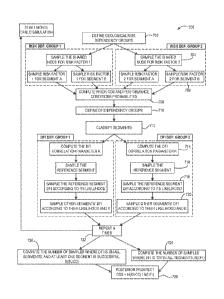
[0096] Figure 7 illustrates a flowchart of a method 700 for determining a
posterior prospect
COS, according to an embodiment. At the prospect level, the geological risk
dependency groups
may be defined, as shown at 702. The shared nodes for the risk factors may be
sampled, as
shown at 704. For segment = sl :sN, rl, rQ
may be sampled according to the shared nodes,
19
CA 02904139 2015-09-03
WO 2014/159479 PCT/US2014/023855
as shown at 706. The prior COS may then be derived. The prior probabilities
may be computed
for each failure scenario. The likelihoods for each success and failure
scenario may be assigned.
The posterior COS1DFI may then be computed using the prior probabilities and
the segment
likelihoods, as shown at 708. The DFI dependency groups may be defined, as
shown at 710.
The segments may be classified as part of (e.g., enrolled in) the DFI
dependency groups, as
shown at 712.
[0097] The DFI correlation parameter k may be computed using the Pearson
correlation
parameter for COS, as shown at 714. For each dependency group, the reference
segment may be
sampled, as shown at 716. The DFI signal for the reference segment may be
sampled using its
likelihoods, as shown at 718. For segment = 1: (Nd-1), (all but the reference
within the
dependency group) the DFI signals may be sampled according to their
likelihoods and to the
sampled DFI signal, weighted with the DFI correlation parameter k, as shown at
720. This
process may be repeated N times, as shown at 722. The number of samples whose
DFI variable
is present in one, some, or each of the segments may be computed, as shown at
724. The DFI
variable present may indicate that the DFI is sampled according to the success
case. The average
volume of these samples gives the "unconditional prospect volume." The number
of samples
that have at least one segment successful, out of the samples selected, may be
computed, as
shown at 726. The average volume of these samples gives the "risked prospect
volume." The
quotient between the number of samples in 726 and 724 may give the posterior
prospect COS, as
shown at 728.
[0098] Embodiments of the disclosure may also include one or more systems for
implementing
one or more embodiments of the method of the present disclosure. Figure 8
illustrates a
schematic view of such a computing or processor system 800, according to an
embodiment. The
processor system 800 may include one or more processors 802 of varying core
(including multi-
core) configurations and clock frequencies. The one or more processors 802 may
be operable to
execute instructions, apply logic, etc. It may be appreciated that these
functions may be provided
by multiple processors or multiple cores on a single chip operating in
parallel and/or
communicably linked together.
[0099] The processor system 800 may also include a memory system, which may be
or include
one or more memory devices and/or computer-readable media 804 of varying
physical
dimensions, accessibility, storage capacities, etc. such as flash drives, hard
drives, disks, random
CA 02904139 2015-09-03
WO 2014/159479 PCT/US2014/023855
access memory, etc., for storing data, such as images, files, and program
instructions for
execution by the processor 802. In an embodiment, the computer-readable media
804 may store
instructions that, when executed by the processor 802, are configured to cause
the processor
system 800 to perform operations. For example, execution of such instructions
may cause the
processor system 800 to implement one or more portions and/or embodiments of
the method
described above.
[0100] The processor system 800 may also include one or more network
interfaces 806. The
network interfaces 806 may include any hardware, applications, and/or other
software.
Accordingly, the network interfaces 806 may include Ethernet adapters,
wireless transceivers,
PCI interfaces, and/or serial network components, for communicating over wired
or wireless
media using protocols, such as Ethernet, wireless Ethernet, etc.
[0101] The processor system 800 may further include one or more peripheral
interfaces 808, for
communication with a display screen, projector, keyboards, mice, touchpads,
sensors, other types
of input and/or output peripherals, and/or the like. In some implementations,
the components of
processor system 800 need not be enclosed within a single enclosure or even
located in close
proximity to one another, but in other implementations, the components and/or
others may be
provided in a single enclosure.
[0102] The memory device 804 may be physically or logically arranged or
configured to store
data on one or more storage devices 810. The storage device 810 may include
one or more file
systems or databases in any suitable format. The storage device 810 may also
include one or
more software programs 812, which may contain interpretable or executable
instructions for
performing one or more of the disclosed processes. When requested by the
processor 802, one or
more of the software programs 812, or a portion thereof, may be loaded from
the storage devices
810 to the memory devices 804 for execution by the processor 802.
[0103] Those skilled in the art will appreciate that the above-described
componentry is merely
one example of a hardware configuration, as the processor system 800 may
include any type of
hardware components, including any accompanying firmware or software, for
performing the
disclosed implementations. The processor system 800 may also be implemented in
part or in
whole by electronic circuit components or processors, such as application-
specific integrated
circuits (ASICs) or field-programmable gate arrays (FPGAs).
21
CA 02904139 2015-09-03
WO 2014/159479 PCT/US2014/023855
[0104] The foregoing description of the present disclosure, along with its
associated
embodiments and examples, has been presented for purposes of illustration
only. It is not
exhaustive and does not limit the present disclosure to the precise form
disclosed. Those skilled
in the art will appreciate from the foregoing description that modifications
and variations are
possible in light of the above teachings or may be acquired from practicing
the disclosed
embodiments.
[0105] For example, the same techniques described herein with reference to the
processor
system 800 may be used to execute programs according to instructions received
from another
program or from another processor system altogether. Similarly, commands may
be received,
executed, and their output returned entirely within the processing and/or
memory of the
processor system 800.
[0106] Likewise, the steps described need not be performed in the same
sequence discussed or
with the same degree of separation. Various steps may be omitted, repeated,
combined, or
divided, as necessary to achieve the same or similar objectives or
enhancements. Accordingly,
the present disclosure is not limited to the above-described embodiments, but
instead is defined
by the appended claims in light of their full scope of equivalents. Further,
in the above
description and in the below claims, unless specified otherwise, the term
"execute" and its
variants are to be interpreted as pertaining to any operation of program code
or instructions on a
device, whether compiled, interpreted, or run using other techniques.
22